Modelling and Simulation of a Hydrostatic Steering System for Agricultural Tractors

Abstract

The steering system of a vehicle impacts on the vehicle performance, safety and on the driver’s comfort. Moreover, in off-road vehicles using hydrostatic steering systems, the energy dissipation also becomes a critical issue. These aspects push and motivate innovation, research and analysis in the field of agricultural tractors. This paper proposes the modelling and analysis of a hydrostatic steering system for an agricultural tractor to calculate the performance of the system and determine the influence of its main design parameters. The focus here is on the driver’s steering feel, which can improve the driver’s behavior reducing unnecessary steering corrections during the working conditions. The hydrostatic steering system is quite complex and involves a hydraulic circuit and a mechanical mechanism to transmit the steering to the vehicle tires. The detailed lumped parameters model here proposed allows to simulate the dynamic behavior of the steering system and to both enhance the understanding of the system and to improve the design through parameters sensitivity analysis.

1. Introduction

Fluid power systems are used in mobile applications to perform several operations, from load handling and hydraulic equipment control, to the translation and steering control of the vehicle. Due to the ever increasing demand for fossil fuels and pollution limits, researchers in the field are strongly committed in the aim to reducing dissipation in this kind of system, and to this end new alternative architectures and solutions are being proposed, regarding the entire hydraulic subsystem in the vehicle, as done in [1], or focusing on some subsystems as the transmission, as done in [2], and even just on the steering system [3]. These works demonstrate how modelling and simulation represent strong and reliable approaches and also have the advantage of allowing a better understanding of the baseline system and of the influence of the design parameters on the system performance.

Steering systems do not only play a role in the determination of the efficiency of the hydraulic circuit of off-road vehicles, but can moreover influence the vehicle dynamic behavior, thus defining its global efficiency in performing one operation. The steering system influences the tire life, the handling and safety behavior and finally the comfort and satisfaction of the driver. It is not surprising therefore that a thorough understanding of the system can be considered a key factor to improve the whole vehicle performance.

Hydrostatic steering is an effective and efficient way to steer heavy vehicles reducing the effort of the driver, in particular for low speed operating conditions. This aspect is especially important in agricultural tractors where high axle loads, large tires and off road terrain are involved, as also stated in [4]. The hydrostatic steering system has to guarantee at the same time the comfort of the driver and the handling of the vehicle, making sure that the vehicle response is following the desired trajectory.

The objective of this paper was to describe the modelling of a hydrostatic steering system of an agricultural tractor and to analyze its behavior from the point of view of the driver effort requested during steering. Other researchers have used the same approach in the past, but this work differs for essentially three reasons: it is focused on agricultural tractors, it aims to analyze mainly the driver effort during steering, and it simulates the steering wheel torque for different sets of design parameters of the hydrostatic steering unit.

Looking at the research works available on the hydrostatic steering for agricultural tractors, the major interest is actually focused on the evaluation of the steering system behavior in order to apply autonomous vehicle guidance applications. In [5] a four-wheel drive tractor is studied with the aim to present a new algorithm for path tracking, based on inverse kinematic modelling; however, no details of the steering system design parameters influence or steering wheel torque trend during a steering maneuver are reported. Vibrations at the steering wheel also represent a critical issue: in [6] the topic is to study the driver comfort with reference to the vibrations during operation; in this case, different agricultural tractors were experimental analyzed and then one of the vehicles analyzed was considered to propose solutions to dampen the vibrations. Again, the focus is different from the one of the present work, in which particular care has been given to the detail level in modelling the steering system. In [7] the focus is the analysis of the role of steering wheel feedback torque in agricultural tractors; this issue arises since the electronic and electro-hydraulic steering systems remove the mechanical connection to the tires but can virtually supply any desired “artificial” torque at the steering wheel. The paper investigates the topic by means of experimental measurement on the vehicle and on a simulator: it concludes that, if the steering is the only effort required from the driver, the feedback torque at the steering wheel may be removed without influencing the steering performance; but, if the driver is also performing any other monitoring task, the feedback torque helps in improving the performance and the effort, by avoiding unnecessary steering wheel corrections performed by the driver when no “reference feedback” is available. This last paper hence states the importance of evaluating the steering wheel torque in a traditional hydrostatic system, because of its importance as a design characteristic of a steering system, and as a key reference in the comparison with electro-hydraulic power systems.

The complexity of the hydrostatic steering system in agricultural tractors, the high number of design parameters that influence its performance and the different tasks to be optimized, make its analysis and through understanding a complex objective. Moreover, this objective requires one to completely detail the hydraulic and mechanical components characteristics and design. Therefore, virtual modelling and simulation represent a convenient approach that provides researchers and designers with a powerful tool to simulate the dynamic behavior, to understand how to modify the design, to highlight the critical issues.

The approach followed in this paper is to develop a detailed physical model of the hydrostatic steering system of the tractor, as has been done in [8,9,10] for on-road vehicles. As a long term task, the model will be also integrated in the complete vehicle simulation model presented in [11], aiming at realizing a virtual design tool that may considerable reduce design analysis and testing costs. Other examples of this approach in modelling, but related to hydraulic power steering system for heavy-duty commercial vehicles, can be found in [12,13]. In particular, in [12] we can find a similar approach to physical modelling, but applied to a different vehicle, a three axle heavy truck: the vehicle is modelled apparently with a full-car approach and some details of the rotary valve of the steering system are analyzed to assess their influence on the vehicle handling performance. Our approach is similar, but focused on an agricultural tractor: we modelled in detail all the components of the hydrostatic steering system but we adopted a “bicycle model” to simulate the vehicle; the sensitivity analysis of the design parameters of the rotary valve is then conducted making reference to the steering wheel torque, which is the torque the driver feels during the vehicle operation.

For the purpose of this paper, which is the understanding of the impact of the design and operating parameters on the steering behavior, in particular on the steering wheel torque trend, the influence of an uneven and off-road terrain profile has been neglected (flat, on road terrain has been considered here) and the front axle of the vehicle has been considered as rigid. This is a limited operating condition of the tractor, but can help to understand better the influence of the steering system parameters, decoupling the effect of the road disturbances from the effect of the geometric and operational parameters. At the same time, it is rather difficult to find in literature information and data that report the influence of the road profile on the steering wheel torque during a working conditions of a tractor, so far as the authors know. In [14] for instance, a model realized through co-simulation between two commercial software are used to study the steering design parameters influence in a multi-axle vehicle, and even if the wheel-ground interaction is considered, a flat road with no disturbances was chosen to perform the analysis. This is due both to the need of decoupling the effects and of reducing the number of the parameters in the sensitivity analysis, which otherwise would result being very complex. From the point of view of the system design, this approach is solid and helps in understanding and improving the design. While approaching, instead, the vehicle analysis and modelling, the handling and the stability, the impact of terrain is a very critical issue and has to be considered. Moreover, since the front axle of the agricultural tractor considered is actually suspended, when implementing an uneven road profile to study its impact on the steering system, also the suspension reaction, which filters the road disturbances, has necessarily to be considered in the model. These aspects will be part of future work, aiming to model all the subsystems of the agricultural tractor to realize a virtual tool able to replicate the experimental tests of the vehicle, performed on the standardized tracks defined by I.S.O. (International Organization for standardization).

In the remainder of the paper, the reader can find a description of the hydrostatic steering system and its operation; a detailed description of the virtual model and of the tuning of the friction parameters; a discussion of the results obtained changing the spring characteristic and flow areas in the rotary valve, and modifying the friction parameters at the steering wheel column and at the mechanical joints of the steering mechanism.

2. Description of the Hydrostatic Steering System and Its Operation

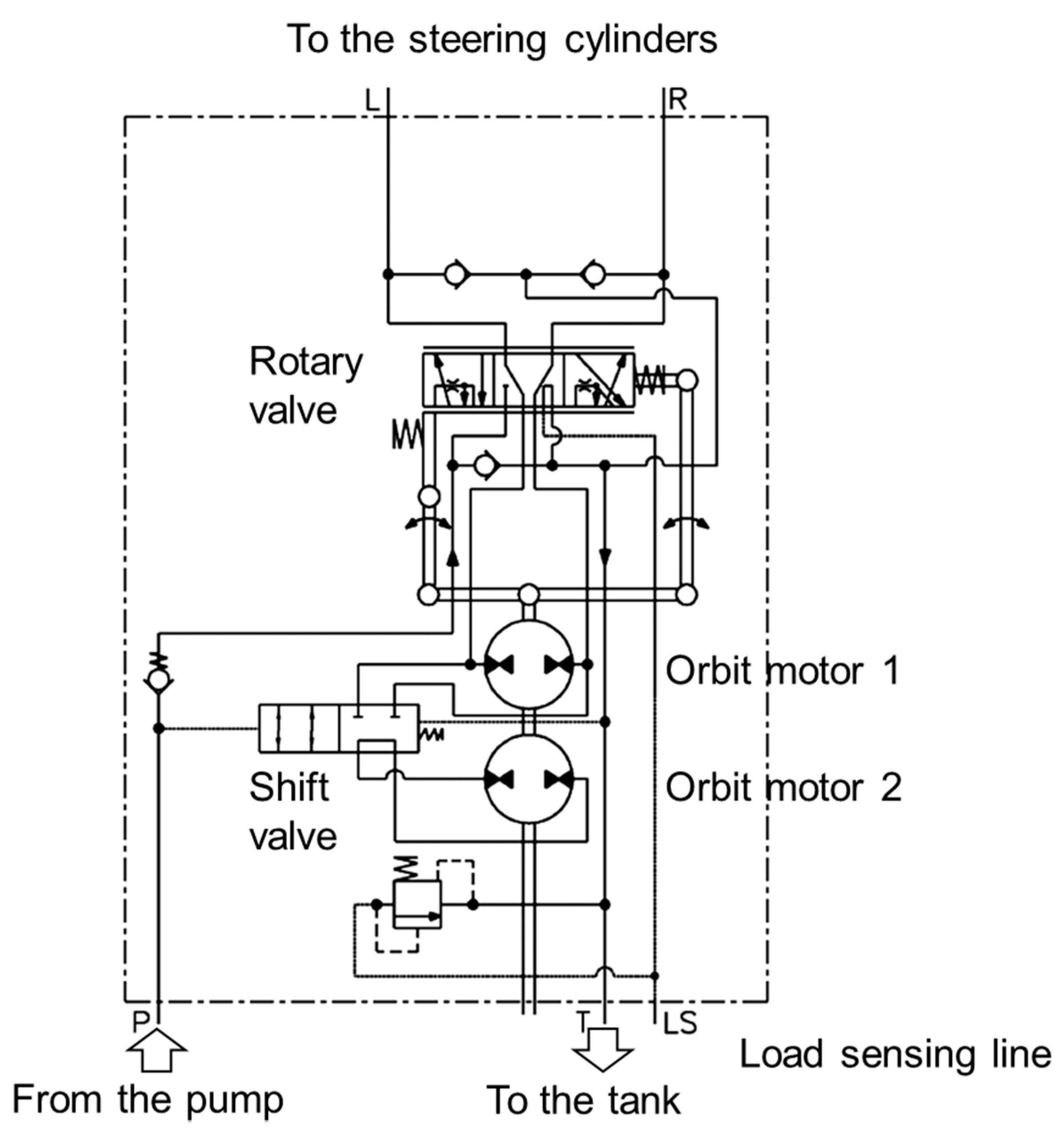
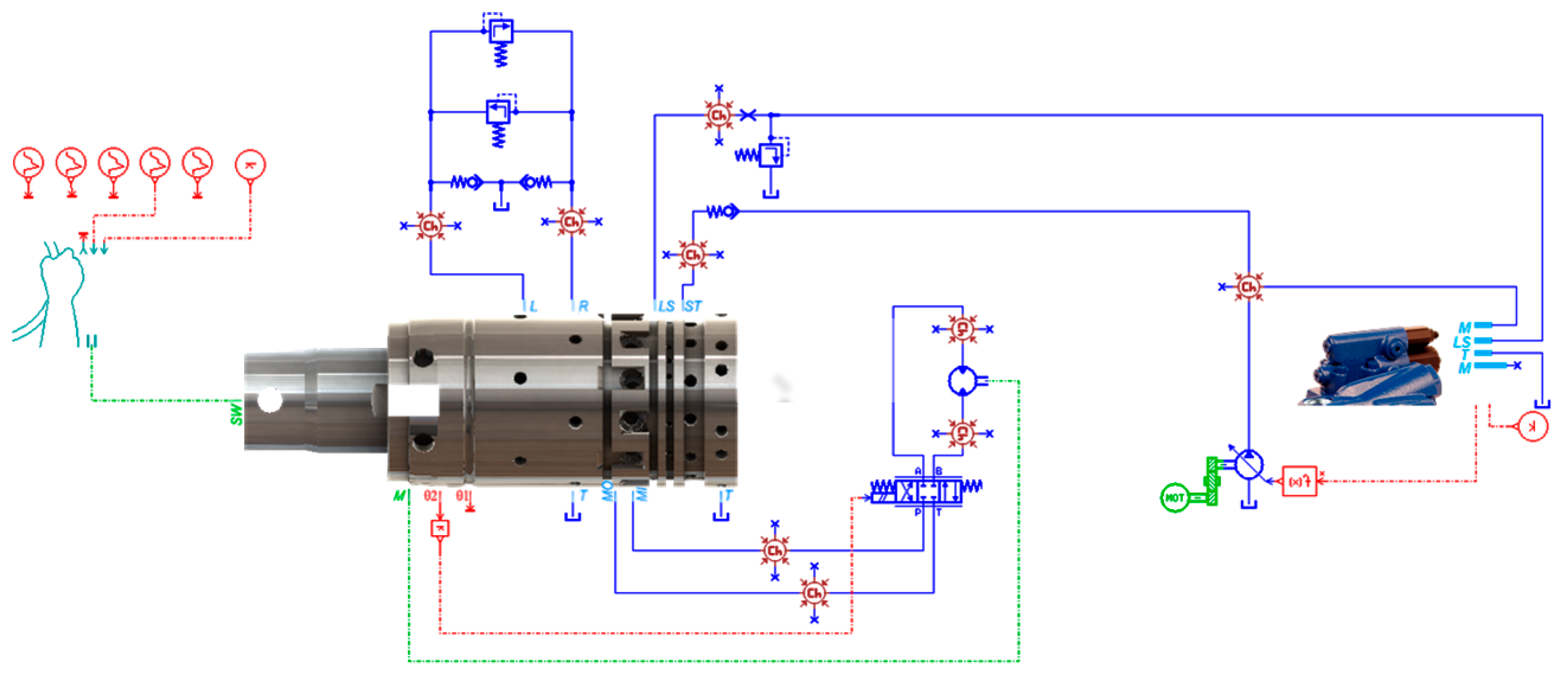
The steering of the agricultural considered tractor (a medium high power tractor) is performed using a hydrostatic unit (Figure 1): the steering wheel column is connected to the spool of a rotary valve, which, once commanded, allows the passage of the fluid from a fluid power unit towards two orbital motors that displace successively the fluid to the steering cylinders (not represented in the schematic but connected to ports L and R). The orbital motors rotate due the pressure difference between the fluid power unit delivery line (minus the pressure losses on the rotary valve) and the steering cylinder pressure. These cylinders are connected to the steering mechanism and perform the steering of the vehicle tires. The hydrostatic steering is hence a servo-mechanism, in which the input given by the driver in terms of mechanical power is amplified as hydraulic power available at the steering cylinders.

A fundamental feedback action is performed by the orbital motor, which, as soon as it begins to displace fluid, also moves the sleeve of the rotary valve in a way to follow the rotation of the spool. Thanks to this feedback movement of the sleeve, the connections with the steering cylinders are closed and they stop moving, performing the partial steering of the vehicle tires according to the input of the driver. If the driver wants to steer more, he has to rotate more the steering wheel, thus causing a new re-opening of the rotary valve connections, a consequent displacement of fluid by the orbit motors, and finally again the following of the sleeve of the rotary valve to close the connections. 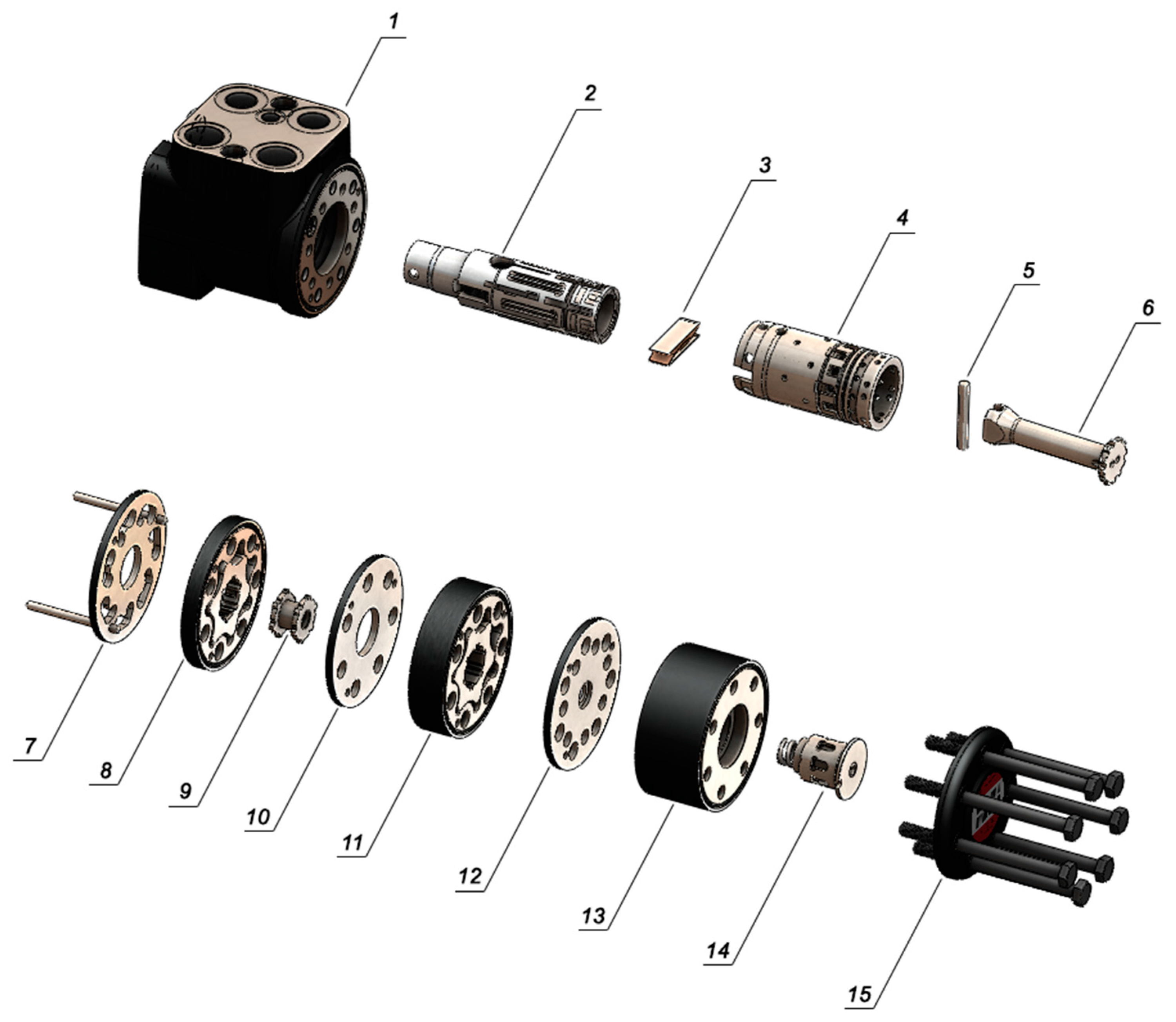In Figure 2 the hydrostatic unit components are shown: the steering wheel column is connected to the spool (2) of the rotary valve; between the spool (2) and the sleeve (4), a pin (5) is inserted with a small gap with the sleeve and a much bigger gap with the spool; the pin is used to limit at ±15° the relative rotation between the spool and the sleeve. The neutral position of the spool is obtained thanks to a set of six leaf springs (3), which play consequently a relevant role in determining the steering wheel torque of the driver to open the rotary valve. The pin (5) also allows the connection of the sleeve to the orbital motors by means of a cardan shaft (6); the cardan shaft is connected on the other side to the internal gear of the orbital motor via a grooved shaft profile, with teeth profile suitable for intersecting axes. In that way, when the internal gear of the orbit rotates, the sleeve, via the connection through the cardan shaft, rotates itself.

The connection ports between the hydrostatic unit and the steering cylinders, the fluid power unit and the tank, are realized on the external body (1); the orbital motor ports are connected to the rotary valve by means of internal cavities on the unit body. Moreover, the body also houses check valves to avoid cavitation at the steering cylinders lines. The steering unit houses two orbital motors labeled in Figure 2 with numbers (8) and (11) (60 cm³/rev and 185 cm³/rev, respectively): during normal operation both the orbital motors are working; during an emergency, when the fluid power unit for some reason is not working and the pressure on the delivery line drops under 7–8 bar, the bigger orbital motor (11) is instead isolated thanks to a “shift valve” (13–14). In this condition the steering of the vehicle tires is still possible acting on the steering wheel, which rotates the spool till its end-stop; at this point, continuing the rotation of the steering wheel and thanks to the pin, the spool drags the sleeve in rotation, and the sleeve drags the internal gear of the orbit to rotate itself. The orbital motor is hence operating in this case as a pump, which sucks fluid from the tank thanks to a check valve (positioned between the delivery and return lines in the system) and delivers it to the steering cylinders. Since the torque needed to rotate a positive displacement pump is directly proportional to its displacement, to reduce the effort needed at the steering wheel, instead of acting on the bigger orbital unit the smaller one is used.

The hydrostatic steering unit considered in this work is of “load sensing” and “closed-center” type: the delivery line P is not connected to the tank T in the neutral position; instead, the load sensing line is connected to the tank and induces the load sensing variable displacement pump that feeds the system to regulate the displacement to the minimum. When the rotary valve is opened, the load sensing line is connected to the inlet line going to the steering cylinders (the load), and senses the pressure to the pump, which regulates its displacement to maintain a fixed margin of pressure between its delivery line and the load.

Moreover, the hydrostatic unit is of the “reactive type”, meaning that the ports towards the steering cylinders side and the ports towards the orbital motors in the unit are connected in the neutral position of the rotary valve. For this reason, the vehicle tires can steer even when the rotary valve is in neutral position, as a consequence of the forces that the ground transmits to them. These forces can pressurize one side or the other of the steering cylinders, and consequently the orbital motor rotates and displaces fluid from a cylinder chamber to the other.

The hydrostatic steering reduces consistently the driver’s effort required at the steering wheel to perform the operation; anyway, some problems may arise: one of the main critical issues is the driver’s feel at the steering wheel that is not always coherent with the vehicle maneuvers.

In fact, depending on the design characteristics of the steering unit and on the geometry of the steering mechanism, the steering wheel torque requested during a steering maneuver may be characterized by sudden variations when changing the steering direction. Moreover, the steering torque needed to perform the complete steering of the vehicle tires may decrease during steering as a combination of the self-aligning moment at the vehicle tires and of the pressure variation in the steering cylinders, thus being in contrast with the increasing of the lateral force on the vehicle. Knowing the steering wheel torque-steering wheel angle trend and the ability of relating it with the geometry of the system is a fundamental step to understand the steering behavior and to propose an eventual design modification.

3. Details and Modelling of the Components

The simulation model of the system is realized in LMS Imagine.Lab Amesim (LMS Imagine Lab Amesim, Plano, TX, USA) [15], a commercial software to perform lumped modelling, particularly suitable for the dynamic analysis of complex engineering systems. The different parts of the system—mechanical, hydraulic and the control parts—are considered in the model and can communicate with each other exchanging compatible variables; for each element a mathematical model describes through opportune equations the element behavior. The lumped parameters model of the hydrostatic steering system, is hence composed of:

-

the rotary valve and the orbital motors

-

the steering cylinders and mechanism

-

the fluid power generator group and priority valve

-

a simplified model of the vehicle

In the following all these subparts are described in detail.

3.1. Rotary Valve

The rotary valve is a directional valve realized by means of a rotary spool and a moveable sleeve. The flow areas that appear and disappear, as a consequence of the reciprocal angular position of these two components, allow the fluid to flow to the orbital motor and then to be delivered to the steering cylinders. Therefore, they are the fundamental design elements of the hydrostatic steering unit and influence the behavior of the steering and the feeling on the steering wheel controlled by the driver. The model of the rotary valve is built using variable hydraulic orifices connected in parallel to represent each of the flow passages through the valve; the flow rate contributions Q_i through the orifices are modelled as in Equation (1), where A_i is the flow area, per_i is the wet perimeter of the orifice section, Δp_i the pressure drop across the orifice, ρ the fluid density and μ the dynamic viscosity, v the fluid velocity, D_h,i the hydraulic diameter, C_d,i the discharge coefficient:

$$Q_i=C_{d,i}\cdot A_i\cdot \sqrt{\frac{2\cdot \left|\Delta p_i\right|}{\rho }}\cdot sign\left(\Delta p_i\right),C_{d,i}=C_{\infty }\cdot \tanh \left(\frac{2\cdot {\lambda }_i}{{\lambda }_{cr}}\right),{\lambda }_i=\frac{\rho \cdot v\cdot D_{h,i}}{\mu },D_{h,i}=\frac{4\cdot A_i}{pe{r}_i}$$

(1)

In Equation (1) the discharge coefficient C_d,i is defined as function of the Reynolds number value λ_i calculated during simulation, of the critical Reynolds number value λ_cr, i.e., the value for which the flow is supposed to transform from laminar to turbulent, and of the asymptotic value of the discharge coefficient C_∞, which is the value reached by the discharge coefficient in fully turbulent flow condition.

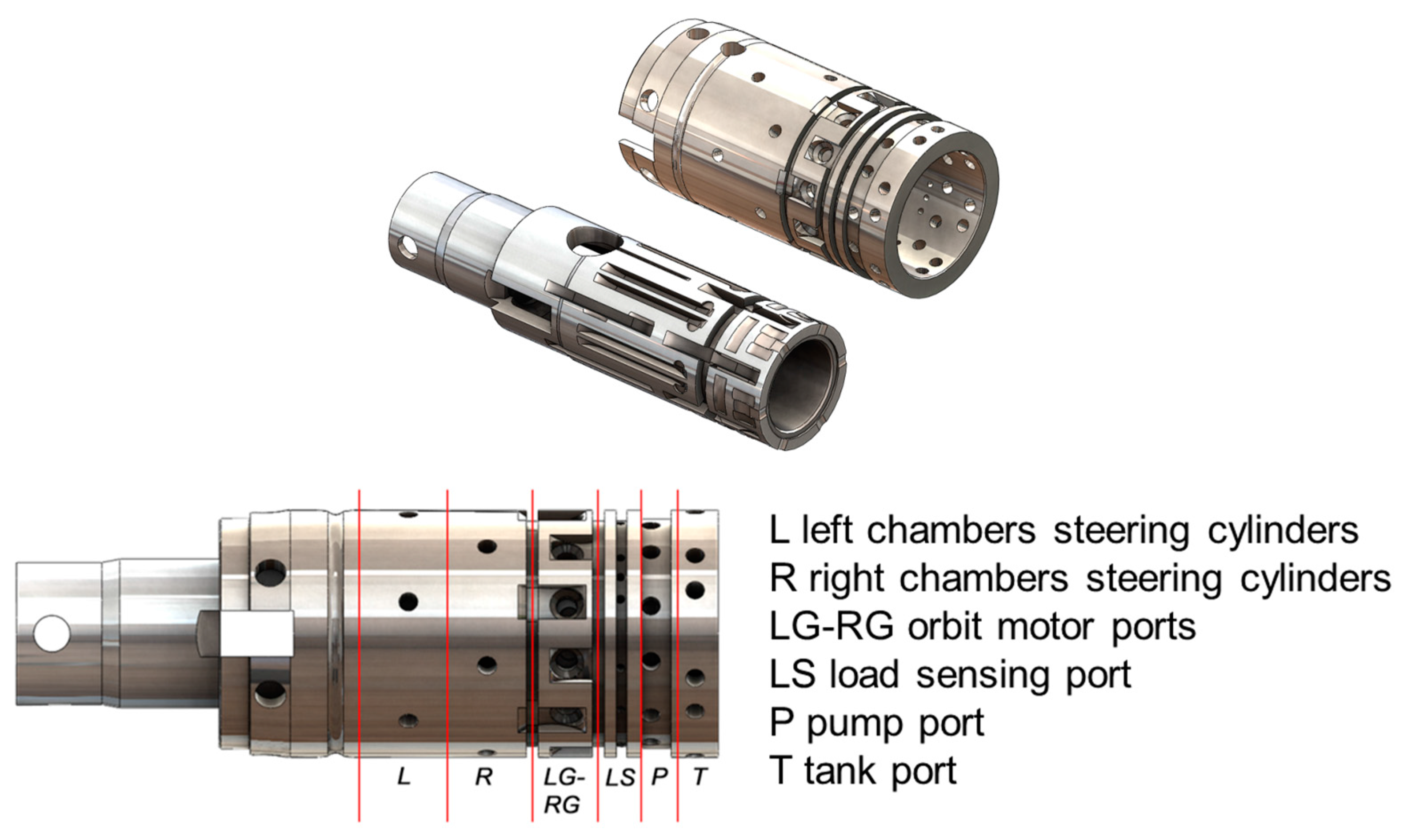
However, the rotary valve has a quite complex geometry and the problem to define the aforementioned flow areas is not trivial. It was decided to perform a reverse engineering on a real component, by means of a 3D laser scanner, in a way to build the 3D CAD (Computer Aided Design) model (SolidWorks, Waltham, MA, USA) used later to define the flow areas. This has required three different scan sessions of the sleeve and spool, whose scans are opportunely aligned and merged to obtain a unique model, as visible in Figure 3.

Managing the 3D model in SolidWorks (SolidWorks, Waltham, MA, USA) and using the Application Programming Interface (API), it was possible to automatize the definition of the flow areas that arise from the superimposition of the holes in the rotating sleeve and the slots on the rotary spool. A macro written in Visual Basic for Applications (Microsoft Corporation, Redmond, WA, USA) was realized with the aim to automatically rotate the valve sleeve with respect to the spool and to identify and calculate the flow areas for each angular step defined, according to the method already presented in [16].

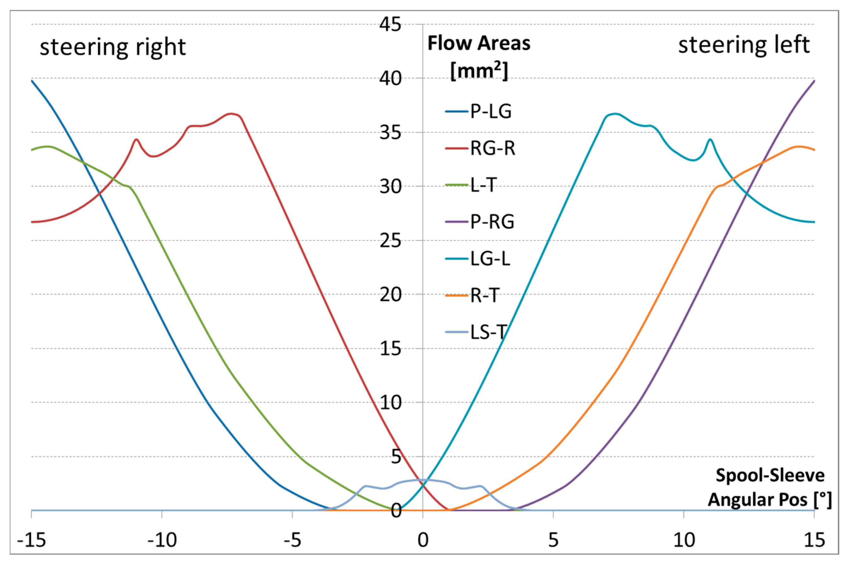
For the analysis performed, the angular interval considered in the reciprocal position of the spool and the sleeve is [−15°; +15°] and a step of 0.05° has been adopted. Making reference to the nomenclature presented in the previous section and in Figure 3, the following Figure 4 shows the total flow areas trends—obtained summing each contribution for any type of connections—as a function of the relative angular position.

Some comments arise looking at the total flow area trends:

-

In the centred position, the connections between the orbit motor and the cylinders are open (flow areas RG-R and LG-L) meaning that this is a reactive load sensing hydrostatic steering unit; moreover, the load sensing line is connected to tank in this position;

-

Steering right, i.e., moving towards a negative relative angle between the spool and the sleeve, the flow area LG-L between the left chambers of the two cylinders and the orbital motor closes and soon after the left chambers are connected to tank; an overlap of 0.5 [°] exists between these areas. At the same time, the flow area RG-R between the right chambers of the steering cylinders and the orbit motor increases.

-

Successively, the flow area P-LG between the pump and the orbital motor opens and the steering cylinders can finally move (LG is hence the inlet orbit port, RG the outlet orbit port). The area LS-T between the load sensing line and the tank closes at this point and the load sensing line is pressurized with the pressure of the right chambers of the cylinders. The flow areas P-LG and LS-T have an overlap of 1°.

The system behaves in similar way when we steer left, as shown by the mirrored trend of the flow areas for positive relative angle between the spool and the sleeve. In the model, the rotary valve flow rate passages open and close as a function of the relative angular position between the spool and the sleeve. This is calculated comparing the dynamic angular position of the spool, directly determined by the steering wheel, and the angular position of the sleeve, which follows the spool to regain a neutral position in the valve.

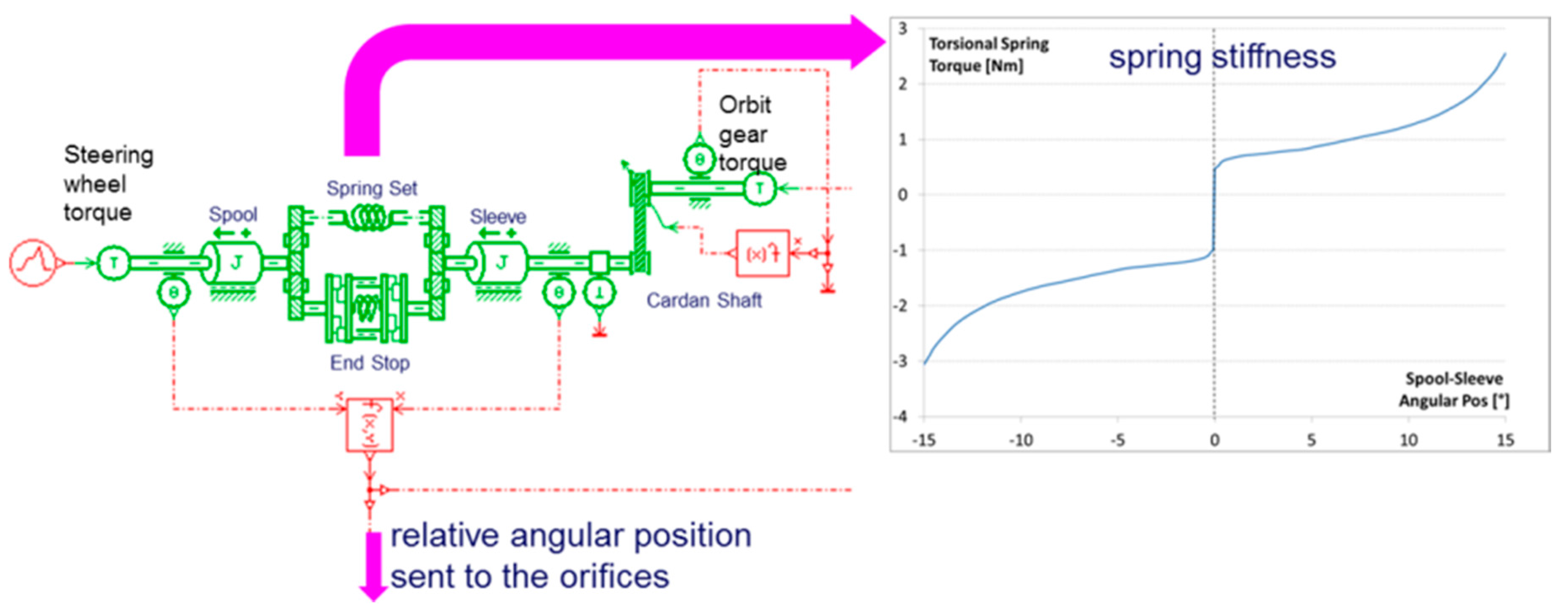
The set of leaf springs determines the relative position of the two elements. Equation (2), where the angular acceleration is named ${\ddot{\theta }}_k$, allows to calculate the angular positions θ_k of the two elements are hence calculated through:

$$J_k\cdot {\ddot{\theta }}_k={\displaystyle \sum _i{M}_{k,i}}$$

(2)

where J_k is the inertia moment of the sleeve (k = 1) or the spool (k = 2), while M_k,i are the torque contributions acting on the two components. For the spool, these contributions are the driver torque on the steering wheel, the friction torques, the reaction of the spring; for the sleeve they are the spring reaction, the friction torques and then the resistance torque of the orbit motor, transmitted by the cardan shaft.

The springs contribution is however the main one and springs with different characteristics influence the driver’s steering feel. In Equation (3) the ratio between the sleeve angular velocity, ω_sleeve, and the cardan shaft angular velocity, ω_cardan, i.e., the transmission ratio, is shown; α is the angle between the intersecting axes of the cardan shaft and the sleeve and ϕ is the angle of rotation of the internal gear of the orbit motor, connected to one end of the cardan shaft:

$$\frac{{\omega }_{sleeve}}{{\omega }_{cardan}}=\frac{\cos \alpha }{1-{\left(\cos \varphi \right)}^2\cdot {\left(\sin \alpha \right)}^2}$$

(3)

Figure 5 displays the model of the two interconnected rotary inertias of the spool and the sleeve. The rotary valve is controlled via a signal generated in the Steering Wheel Actuator Component of the AMESim library “vehicle dynamics”. Inside this component, a P.I.D. (Proportional-Integral-Derivative) controller is used to chase the steering wheel angular position (i.e., the input), giving as output the corresponding torque at the steering wheel, which is used as an input by the spool rotating inertia. The rotary valve in the model is connected to the fluid power generator unit and to the steering cylinders via hydraulic ports, through which flow rate and pressure are exchanged.

3.2. Orbit Motors

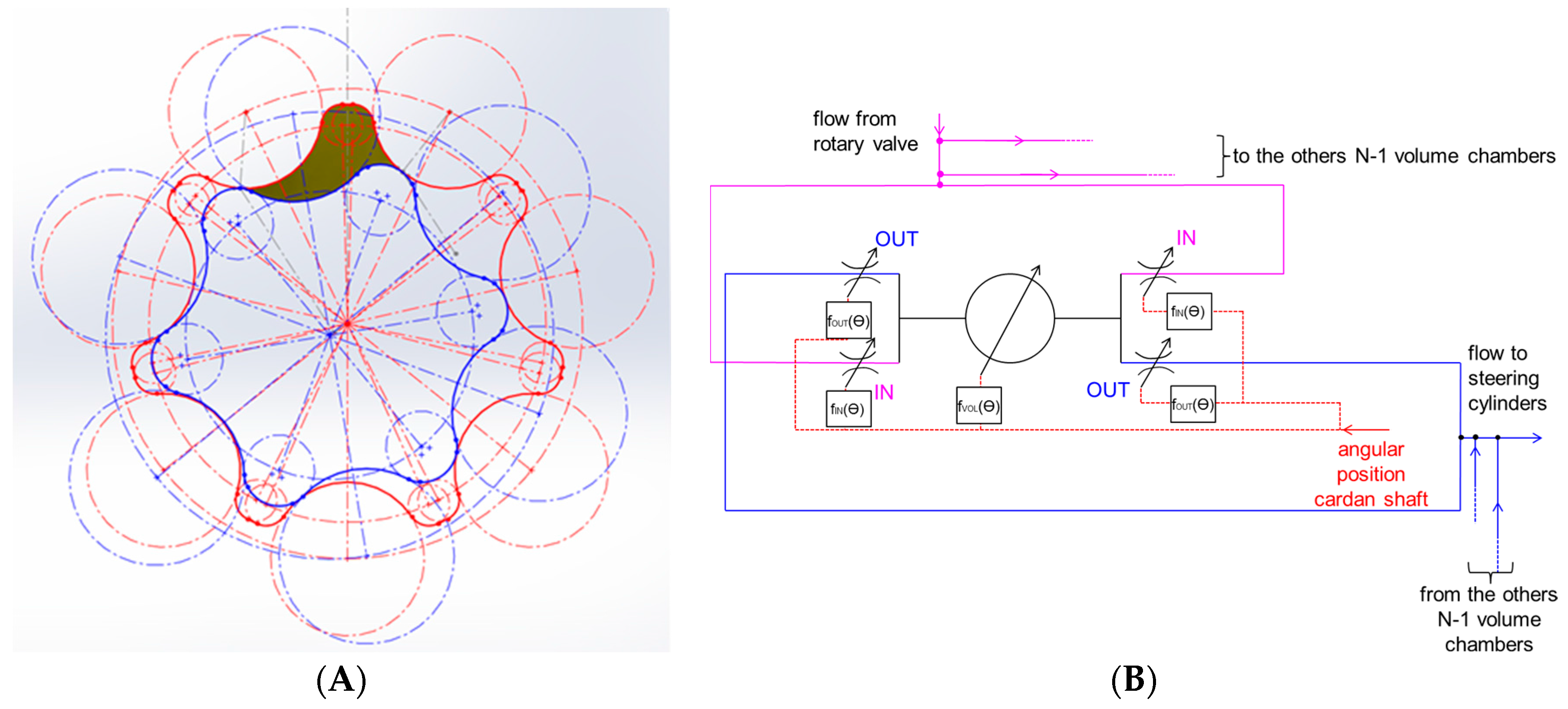
The two orbital motors have the same gears, but different gear face width, thus making one orbit more than the double in displacement than the other. The lumped parameter model of the orbital motor was designed following the typical lumped parameters approach adopted for positive displacement machines, as for example in [17,18]; the internal (N − 1 teeth) and external gears (N teeth) define, while rotating, N volume chambers, which are cyclically connected with the rotary valve side (the inlet from the point of view of the orbital motor) and the steering cylinders side (the outlet from the point of view of the orbital motor). After building the CAD model of the two gears, on the basis of the geometrical parameters, it is possible to calculate the volumes and connection flow areas for a chamber during a whole cycle of the orbital motor.

A single hydraulic chamber (displayed for example in Figure 6A), defined between the internal and external gears, performs an entire cycle (from the minimum volume to the maximum volume and again to the minimum) when the internal gear, which is connected to the cardan shaft, has rotated of 360°/(N − 1). During this angular interval the chamber is connected via the rotary valve to the inlet port and, successively, to the outlet one. Two sets of variable restrictors are used to connect the chamber to the neighboring ports, to consider the bi-directional rotation of the gear; hence, for negative angles of rotation of the spool and orbit internal gear, a set of IN and OUT restrictors is open and the other one is closed and vice versa for positive angles. Every restrictor and the volume chamber are controlled by a function of the angle, and their trends are obtained from the CAD model of the orbit gears and port plate. In Figure 6B the symbolic model of an inter-teeth chamber is shown.

Applying and solving continuity Equation (3) in the volume chamber it is possible to determine the pressure transients p_i inside the chamber as function of the angular position θ_i. In Equation (4) V_i represents the chamber volume evolution, B the fluid bulk modulus, Q_j the flow rate contributions exchanged with the inlet and outlet ports, ω the angular velocity of the internal gear. As a consequence, also the total instantaneous flow rate at the inlet and outlet ports and finally the torque contribution at the cardan shaft are known. All these variables are computed as function of the orbit internal gear angular position:

$$\frac{d{p}_i}{d{\theta }_i}=\frac{B}{\omega \cdot V_i({\theta }_i)}\cdot \left({\mathrm{\Sigma }}_j{Q}_j-\omega \cdot \frac{d{V}_i}{d{\theta }_i}\right)$$

(4)

The orbital motors are connected to the rotary valve with hydraulic ports, through which they exchange pressure and flow rate.

3.3. Steering Mechanism

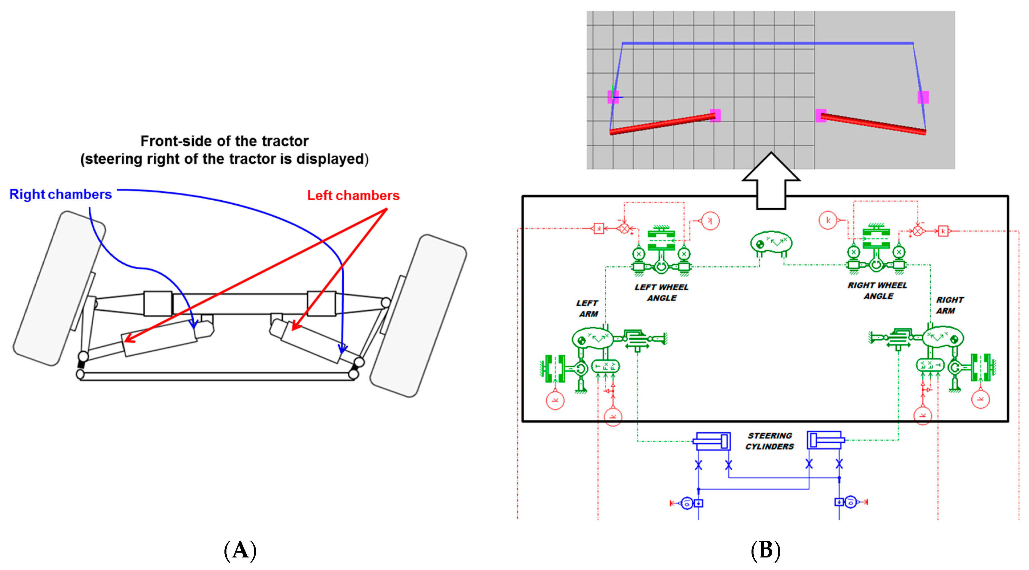
The steering system adopted on the front axle of the agricultural tractor is an Akermann mechanism, with two hydraulic double acting differential cylinders connected as in the following Figure 7A. In the model, the mechanism has been considered planar and the cylinders have been consequently geometrically adapted with respect of the real system, in a way that the cylinder displacements generate the same steering in the model as in the reality. Making this simplification, we used the planar mechanical approach to model the mechanism, connecting rigid bodies and joints as in Figure 7B.

Due to the use of differential-area cylinders and their connection, and due to the steering mechanism too, the volume of fluid displaced for steering left is not equal to the volume of fluid needed to re-align the wheels, hence the steering wheel angle intervals needed to steer the tires and to re-align them are not exactly the same.

In the model, the steering mechanism is connected to the steering cylinders through mechanical ports (they exchange force, displacement and linear speed) and to the vehicle model, receiving from it the torque on the front tires and returning to the vehicle model the angular position of the front tires.

3.4. Vehicle Model

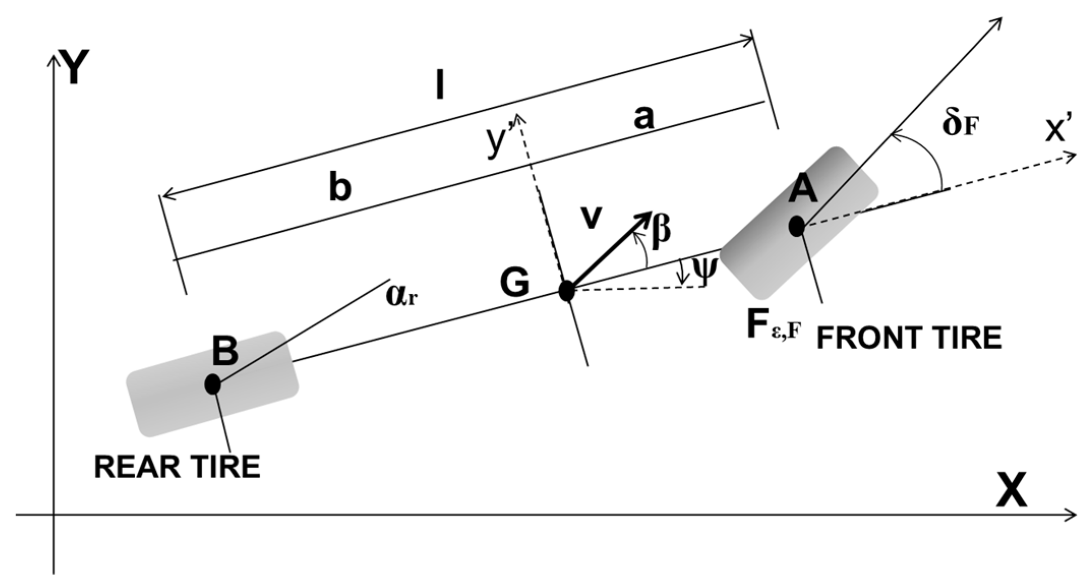
The vehicle is modelled adopting the kinematic bicycle model. In this model the right and left tires at each vehicle axle are supposed to behave the same and are lumped in only one element; no suspension is considered on the front axle; the vertical displacement, pitch and roll rotations of the vehicle are not considered. It has two degrees of freedom: the yaw velocity $\dot{\psi }$ ($\psi$ is the yaw angle) and the side slip angle β between the velocity v of the centre of mass G of the vehicle and the vehicle longitudinal axle. The model is frequently used to analyze the steering behaviour of the vehicle and gives reliable results especially when no higher lateral accelerations are involved in the vehicle operation [19]. If only the front tire can be steered, and δ_F is the steering angle, the model is represented as in Figure 8 and by Equation (5), whose symbols are shown in figure.

$$\begin{array}{l}X=v\cdot \cos (\psi +\beta \left({\delta }_F\right))\\ Y=v\cdot \sin (\psi +\beta \left({\delta }_F\right))\\ \psi =\frac{v}{b}\cdot \sin \left(\beta \left({\delta }_F\right)\right)\\ \beta \left({\delta }_F\right)=\arctan \left(\tan \left({\delta }_F\right)\cdot \frac{b}{l}\right)\end{array}$$

(5)

Moreover, the model integrates the tire and its interaction with the ground: in particular, it takes into account of the self-aligning torque; this torque, which is due to the friction at the ground and deformation of the tire that generates a lateral force, tends to re-align the tire towards the direction according to which the tire is rolling.

3.5. Fluid Power Unit and Priority Valve

A fluid power unit made of a load sensing variable displacement pump is used in the tractor to feed the steering system; anyway, this pump is also delivering to other utilities, hence different shuttle valves select the highest pressure and send it to the pump and a priority valve, mounted in the pump delivery line, guarantees priority at the steering system with respect to the others. The pump is modelled as an ideal variable displacement pump in which two compensators are integrated to control the displacement: a pressure compensator, set at the maximum pressure value, and a differential pressure compensator, which performs the load sensing control.

4. Model Calibration

The steering unit was first simulated on a virtual test rig, which reproduces the experimental test rig used to test the unit in a previous work [20]. The comparison between experimental and simulation data has been performed with the main aim of setting the friction parameters (viscous friction, static and dynamic friction on the spool and sleeve rotational inertia components) in the coupling between the spool and the sleeve, since these parameters are not known and also change with the operational conditions. According to the test rig layout, the steering unit delivers fluid towards two relief valves, which are used to set the working pressure alternately on the left and right side of the unit (Figure 9). The input is given as linear variation of the steering wheel angle, in a way to produce a complete revolution on one side and to come back. The input is performed in different time interval, thus resulting in different rotational speed values on the steering wheel.

The tested operating conditions are shown in

Table 1. Operating conditions tested in the test rig.

Cracking Pressure Relief Valves(bar)	25, 50, 75, 100, 125, 150, 175
Speed (rpm)	1, 10, 20, 50

.

The comparison between experimental and numerical data was developed looking at the average torque needed to steer, which is constant with a constant rotational speed at the steering wheel. The numerical and experimental data in

Table 2. Comparison between the measured and numerical torque at the steering wheel.

Steering Wheel Speed (rpm)	Experimental Torque to Steer Clockwise (Nm)	Experimental Torque to Steer Anti-Clockwise (Nm)	Average Experimental Torque (Nm)	Average Numerical Torque (Nm)	Error on the Average Torque on the Numerical-Experimental Comparison (%)
1	1.341	0.813	1.077	1.097	1.8
10	1.393	0.885	1.139	1.149	0.9
20	1.399	0.988	1.193	1.209	1.4
50	1.701	1.243	1.472	1.478	0.4

show the dependency between the speed at the steering wheel and the torque: as expected, the higher the steering wheel speed is, the higher the relative rotation of the spool with respect to the sleeve is; this generates also the opening of greater connection areas between the steering unit and the steering cylinders, resulting in an bigger steering angle at the vehicle tires too. Since this is obtained opening more the rotary valve, it implicates also that the spring between the spool and the sleeve has to be compressed more, requiring a higher torque also at the steering wheel.

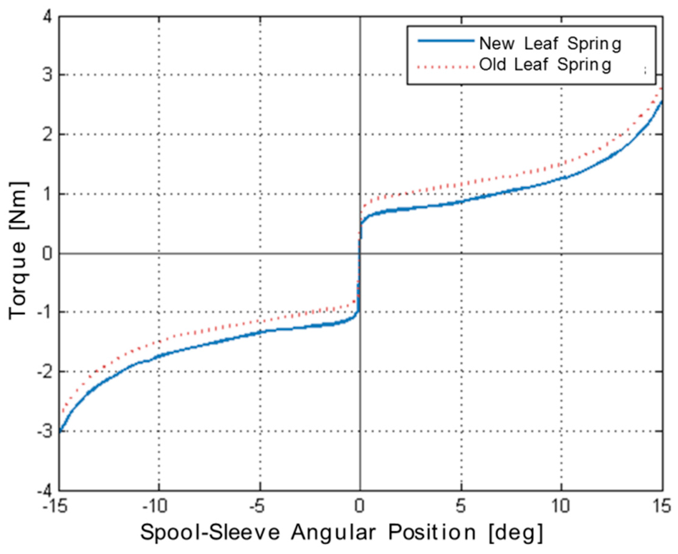
The setting of the friction contributions in the model is chosen to obtain a good comparison between the experimental and numerical torque values. However, the experimental data show a non-symmetry in the steering unit behaviour when steering clockwise and anti-clockwise. This is probably due to a non-ideal behaviour of the spring, which has lately been represented in the model using the non-symmetric characteristic curve; in Figure 10 the two characteristics of the spring, the original one and the modified one, are displayed.

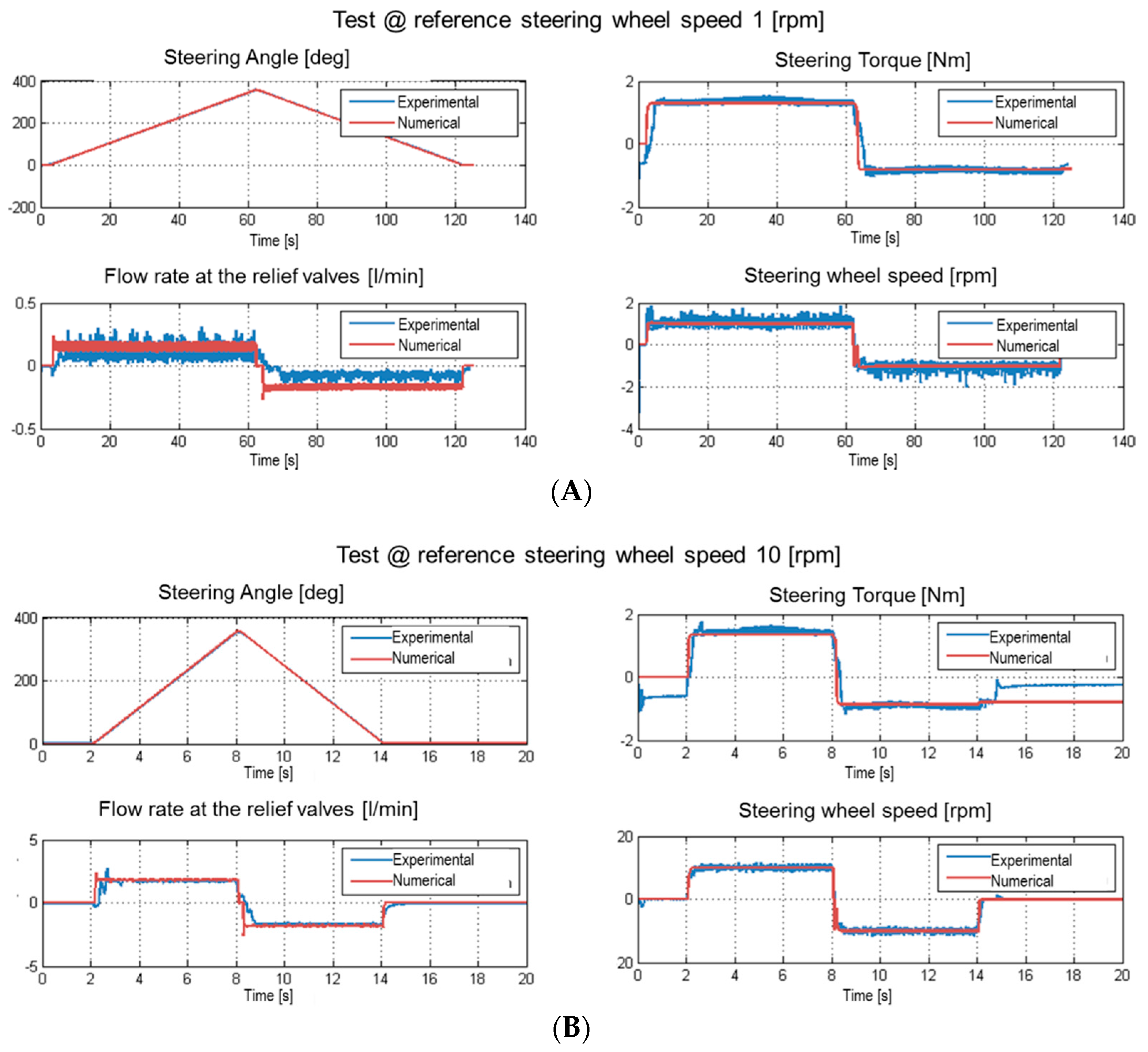
Moreover, a complete set of data for two different wheel speed values are shown in Figure 11 to demonstrate consistency between the behaviour of the numerical model and the experimental behaviour.

5. Results

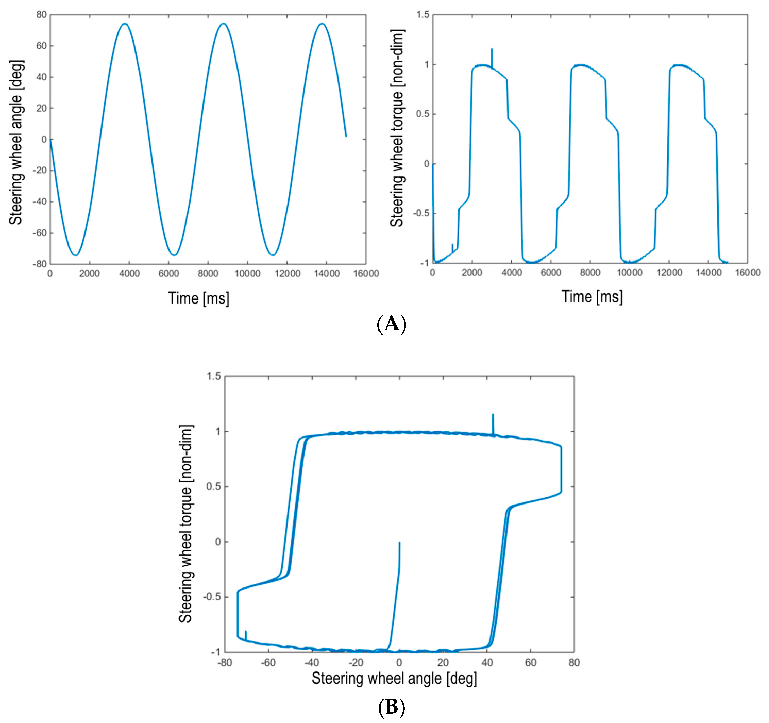
The first main result of the simulation model is its ability to perform a complete steering manoeuvre: the desired angular position as a function of time at the steering wheel is given as input; a sinusoidal shape is used to replicate approximately a real steering manoeuvre, while the vehicle is moving at a constant speed. The complete model previously described is here used to determine the steering characteristics and the influence of some of the main geometrical and design parameters on its behaviour. In the next figure this characteristic curve, as calculated by the numerical model previously described, is shown considering the baseline model setting and considering a sinusoidal fashion for the input steering wheel angle with frequency of 0.2 Hz and amplitude of 75°, as shown in Figure 12A, together with the non-dimensioned torque. The steering wheel torque is non-dimensioned with respect to the maximum torque obtained with the baseline setting. In the several tests performed, the tractor is supposed moving at intermediate constant speed value (about 30 km/h).

At the beginning of the steering manoeuvre, the steering torque rises rapidly to the value needed to perform the steering, thanks to the effect of the P.I.D. (Proportional-Integral-Derivative) controller at the input of the steering unit; continuing the steering, the speed at the steering wheel decreases till zero when the maximum angle is reached, and the torque slightly decreases. Reversing the rotation direction at the steering wheel, the effect of the self-aligning moment on the vehicle tires helps them to return in the neutral position without needing a contribution from the steering cylinders; consequently, at first, the torque needed at the steering wheel to perform the manoeuvre is still of the same sign (positive if before it was positive, negative if before it was negative) and changes sign only when the effect of self-aligning moment on the vehicle tires is reduced. At this point the cycle repeats symmetrically with respect to the first part described.

These trends are well in line with the driver’s feel on the real tractor described in the following: while increasing the maximum steering angle, the steering wheel becomes “lighter”; moreover, when the maximum steering angle for a specific steering operation is reached, the driver feels a discontinuity on the torque needed at the steering wheel that is a bit confusing and may provoke opposite reaction in the drivers.

The same results are shown in Figure 12B, where the torque trend is plotted as function of the steering wheel angle and, from this moment on, we will refer to this kind of diagram to compare the obtained results. In the next paragraphs the influence of some of the main design parameters of the steering unit are analysed, in a way to understand how these parameters affect the driver’s feel.

5.1. Influence of the Leaf Spring Between the Spool and the Sleeve of the Rotary Valve

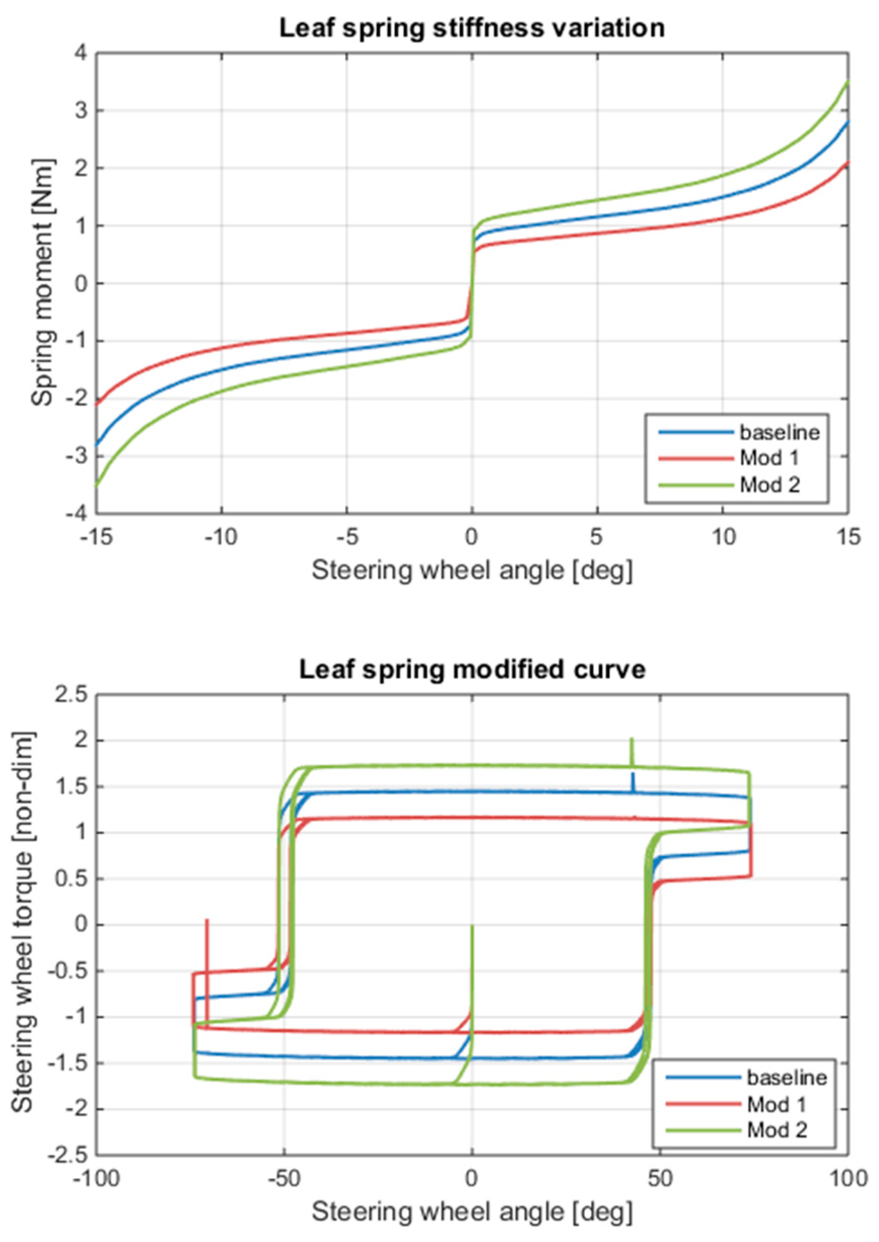
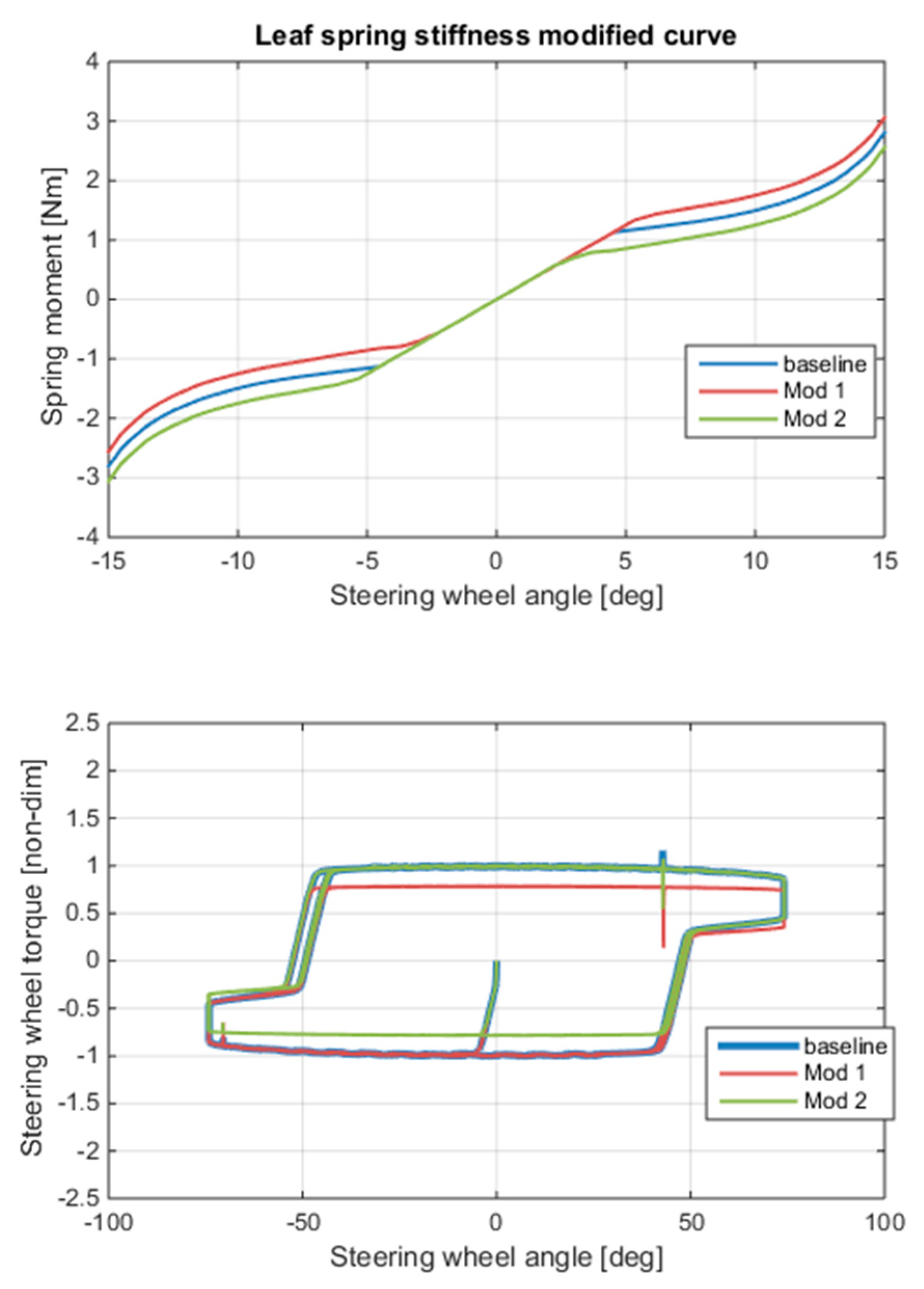
The steering wheel torque trend as a function of the steering wheel angle is shown in Figure 13 for three different leaf spring stiffness, also displayed in the figure. The torque is non-dimensioned with respect to the maximum value of the torque obtained in the baseline simulation shown previously; the input steering angle is still the one shown in Figure 12A. As expected, a smaller torque at the steering wheel is needed if the spring stiffness is lower, hence requiring less effort from the driver.

A second set of simulations has been realized, trying to modify the spring characteristics at the neutral position of the spool of the rotary valve, in a way to influence the steering torque at the transition between a positive and a negative value and vice-versa. In Figure 14 the spring characteristics with this modification and for different values of the stiffness are shown together with the correspondent results on the steering torque trend. With a smoother slope of the spring characteristics, the transition of the torque is more gradual and this may improve the driver’s feel. In that way, changing the spring stiffness in the virtual model, the wheel torque curve is modified and the designer can determine the setting that allows to meet the need of the driver eventually asking for a smoother feedback.

5.2. Friction on the Steering Wheel Column

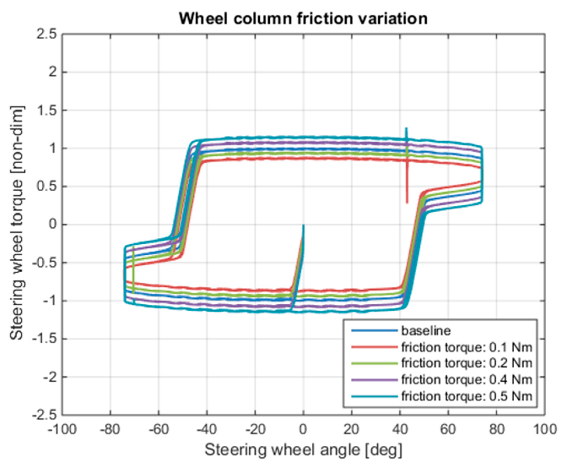
Friction on the steering wheel column directly influences the effort of the driver during steering. As Figure 15 displays, when increasing the friction factors (static and dynamic friction forces) the area enclosed on the steering torque-steering wheel angle diagram increases, since it represents the energy dissipated when performing the operation. Also the step variation of the torque when the steering direction is inverted at the steering wheel increases with the friction.

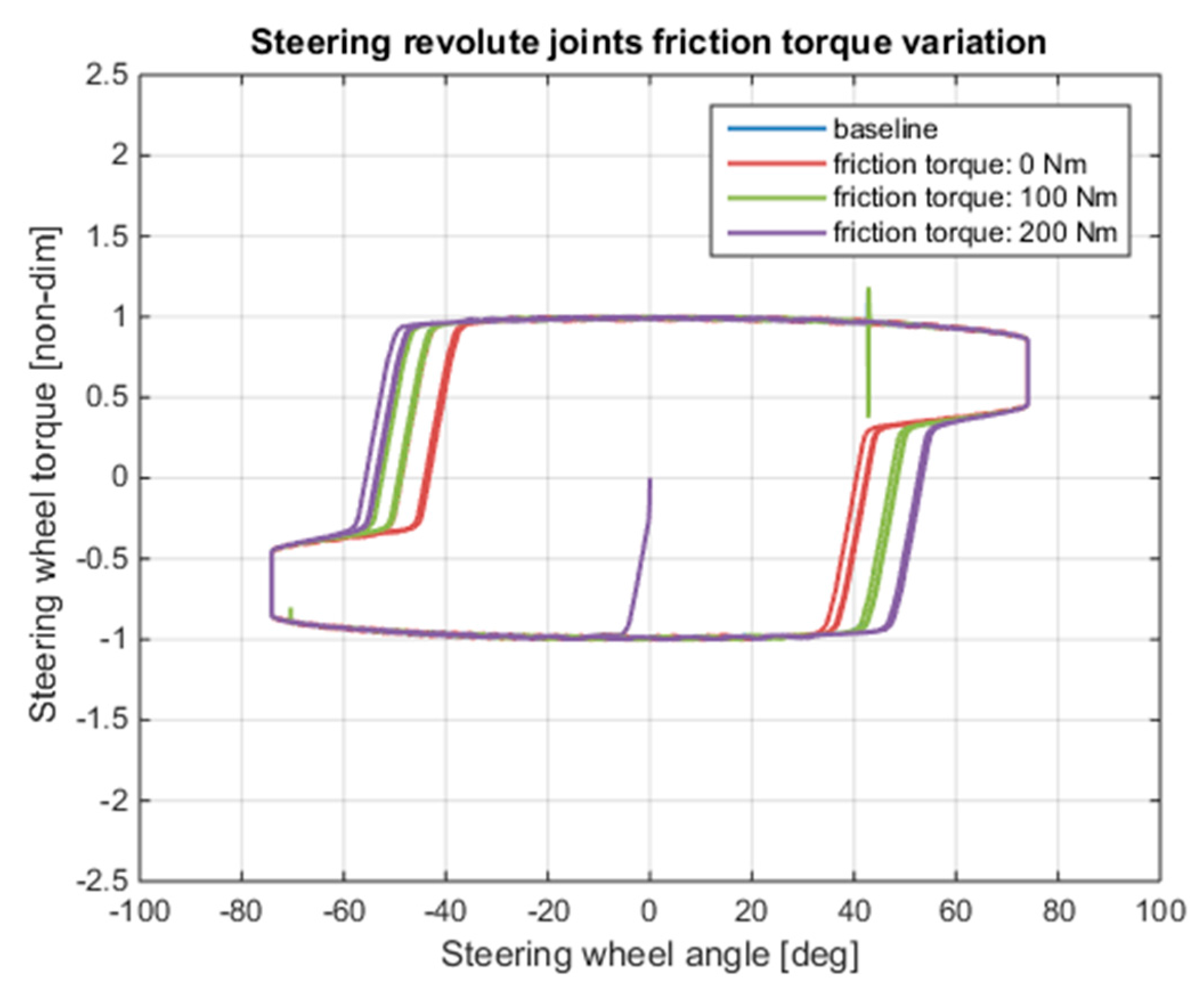
5.3. Friction on Revolute Joints of the Steering Mechanism

In these simulations the friction torque values at the joints between the vehicle front axle and the vehicle tires hub is varied (Figure 16). This has a main effect on the steering wheel torque transition between negative and positive values and vice-versa: with more friction the re-aligning moment of the tires is in part dissipated, hence the driver has to anticipate his effort on the steering wheel (i.e., for lower steering wheel angle) if compared with the baseline setting.

5.4. Flow Areas on the Rotary Valve

The rotary flow areas have been defined with accuracy in the model after the reverse engineering work on the steering unit. At this point little variation in the flow areas are introduced to analyse the influence on the steering behaviour. This kind of analysis may also be used to guide the design of a new rotary valve in which the connections are optimized on the basis of the driver’s feel. With the new potential offered by the additive manufacturing techniques, it is plausible to imagine a next future in which the standard rotary valve geometry can be adapted to the driver’s need when using a specific vehicle typology and performing a specific work on a terrain.

What most influences the steering behaviour is the flow areas opening and closing timing, hence this analysis is focused on this aspect, translating the flow area curves to increase and decrease the overlap. Two different test cases are analysed, with reference to Figure 4.

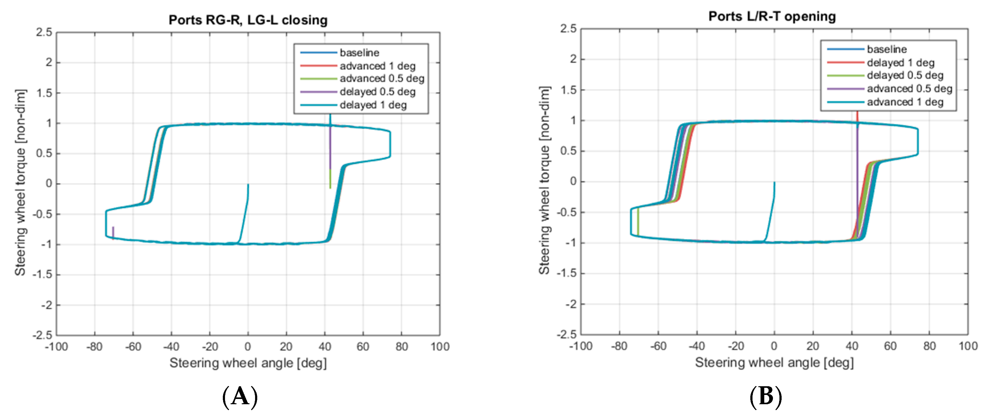
First test case: modification of the overlap between the flow area RG-R and the flow area LG-L (the connections going to the steering cylinders) respectively with flow area R-T and the flow area L-T (the connections between the steering cylinders and the tank).

The overlap is changed first translating the curves RG-R or LG-L, then translating the curve R-T or L-T; since the geometry is not exactly the same in the two cases, different results can be obtained. In the first case, the influence on the steering wheel torque is quite negligible, as it can be seen in Figure 17A. Increasing or decreasing the overlap here simply means that the steering cylinder chambers connected to the tank are discharged a little bit earlier or later (at the beginning PG-R and LG-L are connected because the steering unit is of the reactive typology). This has no greater effect in determining the steering torque, which is more sensitive to the delicate opening connections between the fluid power unit and the steering cylinders.

In Figure 17B the trends shown refer to the variation of the angular interval in which the cylinders are connected to the tank: when increasing the overlap between the flow area RG-R and the flow area R-T—and, on the other side, the flow area LG-L and the flow area L-T connections—by advancing the opening of the connections to the tank, the back-pressure at the cylinders chambers is lower, and the torque transition happens for slightly higher wheel steering angle.

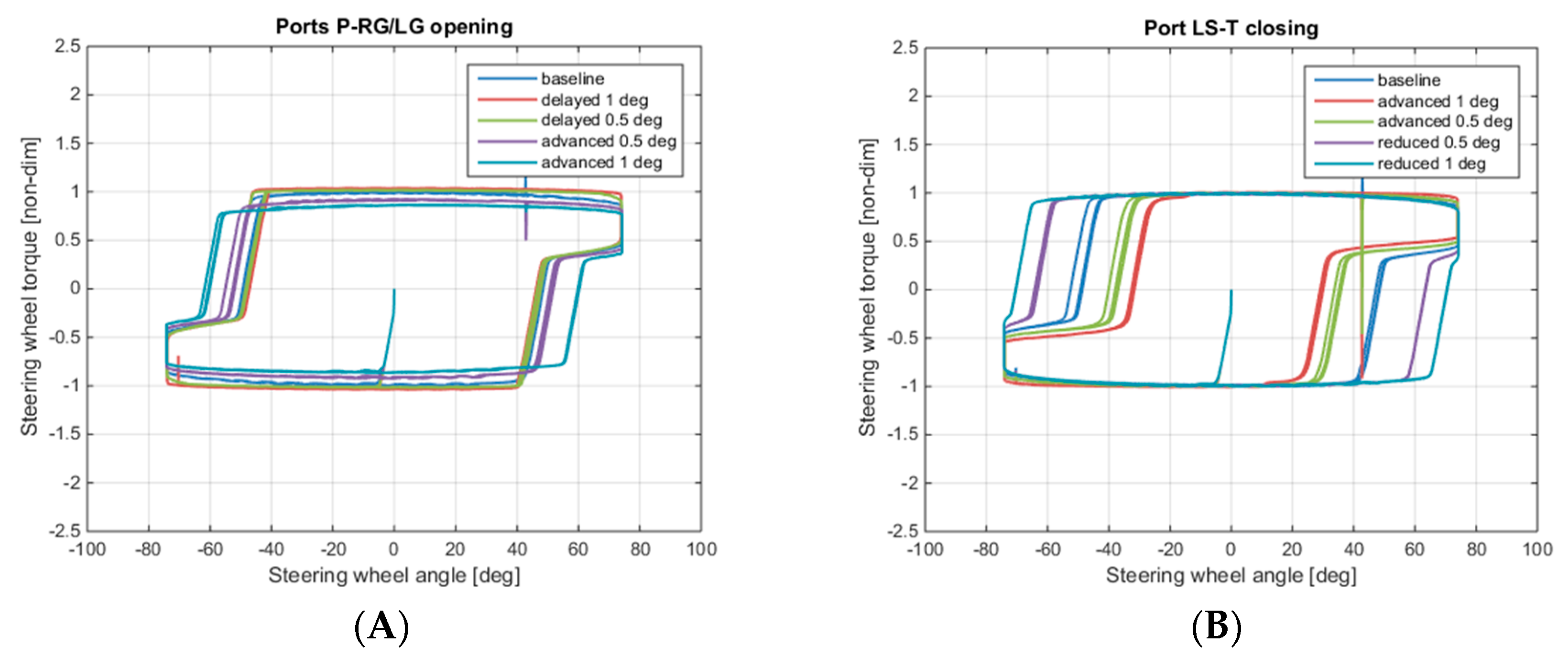
Second test case: modification of the overlap between the closing of the connection LS-T (flow area that allows the load sensing to be connected to the tank with the rotary valve in neutral position), and the connections P-LG and P-RG (flow areas that connect the fluid power generator unit with the rotary valve). The overlap is changed first translating the curves P-RG and or P-LG, then modifying the angular interval during which the area LS-T is open; since the geometry is not exactly the same in the two cases, different results can be obtained.

In the first case (Figure 18A), the overlap is decreased by delaying the opening of flow areas P-RG and P-LG, hence the opening of the connection of the cylinders with the fluid power unit is delayed; the effect is that, during the transition from the maximum steering angle to zero, the torque requested at the steering wheel is higher when looking at the same steering wheel angle and the steering manoeuvre takes less advantage of the re-aligning moment on the vehicle tyres. In the case of continuous manoeuvres during the tractor operation on field, this aspect has to be considered as a factor that can determine the driver tiredness at the end of a day of work.

When the overlap is increased, beside the lowering of the driver’s effort during the transition, another desired effect is happening: the maximum steering wheel torque needed does not decrease while approaching the maximum steering wheel angle but remains constant (with a maximum value very similar to the baseline test case): from the point of view of the driver’s feel, this is a more intuitive behaviour respect to the slight decrease visible in all the other analysed cases. The designer has hence to be aware of the chance of slightly modifying the overlap in a way to better encounter the driver’s opinion to make the handling of the vehicle easier.

Modifying the area LS-T (Figure 18B), in particular reducing the angular interval during which the area is opened, the area enclosed in the diagram steering wheel torque-steering angle decreases. A little reduction in the angular interval in which the LS-T is opened, allows obtaining a more gradual variation of the torque when the direction of steering is inverted, taking advantage of the self-aligning moment on the vehicle tyres and reducing the effort of the driver.

6. Conclusions

A detailed model of a hydrostatic steering system of an agricultural tractor has been described in this work; the steering system is a closed-centre, load sensing, reactive hydraulic steering system. The model has been developed using the lumped parameters approach and it comprises the hydraulic circuit layout of the system, the rotary valve, the steering cylinders, the steering mechanism and a simplified model of the vehicle. The aim of the work was to analyze the steering system behaviour, in particular observing the steering wheel torque needed to perform steering and the influence of some design and operating parameters on this characteristic.

Design parameters of the rotary valve (springs characteristic, flow areas timing) are shown to have a deep impact on the steering wheel torque-angle curve and should be considered while designing the system in a way to meet the need of the driver and eventually to minimize his effort. In particular, changing the timing of the connections between the rotary valve and the steering cylinders or between the load sensing line and the rotary valve, greatly influences the shape of the steering wheel torque-steering wheel angle characteristic. A set of leaf springs with gradually higher stiffness characteristics leave the steering characteristic shape the same but enlarge it, determining higher value of steering wheel torque, needed to perform the same steering operation.

The friction contributions on the steering mechanism and on the wheel column cannot being totally considered design parameters, given the difficulty to control these values during design; however, the analysis done can be useful both during the tuning phase of the model, when the experimental results are compared with the numerical ones, and also in the eventuality of the analysis of critical behaviour in the system. More friction generally requires more steering torque from the driver to perform the same operation but also, in particular the friction at the steering mechanism, influences the steering wheel torque transition from the maximum value in one direction to zero.

From the point of view of a designer or a researcher, the model presented allows to understand the system behaviour, to analyze new designs of the rotary valves and the influence of operating parameters. The hydraulic system model is very detailed and takes into account not only of the design of the components but also of the properties of the fluid, in particular the bulk modulus, density and viscosity, and of the pipes and hoses contribution to the system stiffness.

One aspect that can be improved in the future is the vehicle modelling, kept very simple on this work to highlight the role of the hydraulic components in the system. Furthermore, to analyse the vehicle handling and stability and using the same model of the hydrostatic steering system, a more detailed vehicle model has to be considered. Moreover, in this work, as in many similar works, the impact and role of an uneven terrain is not considered when studying the steering. Since an agricultural tractor deals and works with several environments—from the road, to the field with different kinds of terrain, to snow—this aspect may have a huge impact, especially if the handling and stability of the vehicle are under analysis. Besides, this analysis also requires the introduction in the model of the suspension system of the front axle, which acts as a filter with respect to the terrain disturbances. In the future, this issue will be addressed simulating the terrain as a series of external disturbances on the wheels and analysing the impact on a complete virtual model that comprises the steering system and the suspension system [11].