Feature Reduction for Power System Transient Stability Assessment Based on Neighborhood Rough Set and Discernibility Matrix

Abstract

In machine learning-based transient stability assessment (TSA) problems, the characteristics of the selected features have a significant impact on the performance of classifiers. Due to the high dimensionality of TSA problems, redundancies usually exist in the original feature space, which will deteriorate the performance of classification. To effectively eliminate redundancies and obtain the optimal feature set, a new feature reduction method based on neighborhood rough set and discernibility matrix is proposed in this paper. First, 32 features are selected to structure the initial feature set based on system principle. An evaluation index based on neighborhood rough set theory is used to characterize the separability of classification problems in the specified feature space. By constructing the discernibility matrix of input features, a feature selection strategy is designed to find the optimal feature set. Finally, comparative experiments based on the proposed feature reduction method and several common feature reduction techniques used in TSA are applied to the New England 39 bus system and Australian simplified 14 generators system. The experimental results illustrate the effectiveness of the proposed feature reduction method.

1. Introduction

With the increasing demand of society and economic development, power systems tend to be interconnected and large-scale. However, the disturbance may cause more serious accident such as stability crisis and large-scale blackout in this case, which brings huge economic losses [1]. Therefore, it’s essential to analyze the dynamic security behavior of power system by transient stability assessment (TSA). The main purpose of TSA is to judge if the power system is stable or not while a large disturbance occurs [2]. There are mainly two traditional methods for TSA, including the time domain simulation method [3], and the transient energy function method (direct method) [4]. Based on that, many improved methods and strategies are proposed to handle transient stability contingencies [5,6,7]. The methods mentioned above are based on mathematical models, which are quite precise and reliable to obtain the results. Unfortunately, it takes too much time to simulate for the TSA problem, while the scale of power system is large, which is less appropriate for the requirements of real-time online TSA. Nowadays, with the development of phasor measurement units (PMU) and wide area monitoring systems (WAMS), collecting massive synchronized power system data has become a reality [8,9,10]. Moreover, sample and pattern recognition based machine learning methods provide researchers another feasible path. Owing to the advantages of fast real-time response and high precision, many machine learning-based methods are proposed to solve TSA problems [11,12,13,14,15,16,17,18,19,20], such as probabilistic neural networks [11], core vector machine [12], decision trees [13], extreme learning machine [14], etc.

Machine learning-based methods mainly include three steps: (1) constructing the original feature set and selecting the optimal feature set, (2) structuring and training the classifiers offline and (3) evaluating the classifiers online. A general framework of machine learning-based TSA is shown in Figure 1. In terms of classifiers, there are generally two aspects determining their performance. One is the structure and training mechanism of classifiers; the other is the selection of input features and correlation of feature space. Up to now, most related researches are mainly focus on the construction and structure design of classifiers for higher classification accuracy and there is relatively less attention paid to the feature reduction methods for TSA problems. During the running process of power system, there exists massive state data with little difference, which would generate similar feature samples with high correlation. This may cause reuse of similar data and redundancy of features. In addition, too many superfluous features will not only increase the burden on computation but also have an impact on precision of classifiers. Thus, it’s extremely necessary to study the feature reduction problem of TSA.

There are mainly two aspects to be considered in such problems, including the evaluation index of feature set and the designed feature selection strategy. At present, some valuable work on feature reduction of TSA has been done by the previous scholars; we briefly review as follows. In [16], three methods were designed to obtain a feature reduction: sensitivity index and sensitivity analysis were used to construct an original feature set without redundant features and principle component analysis (PCA) was applied to reduce the input feature dimensions. However, the number of features will increase rapidly as the scale of power systems expands. In [11], correlation analysis (CA) and PCA were used for feature selection, but this method can only measure correlations between features and fails to reflect the relevance between features and classes, which means that there may exist features irrelevant to classification. Moreover, the feature space obtained by PCA may not be as complete as the original one. In [17], a bread-first searching technique based on the separability index was proposed to find an optimal feature set which considers correlation between features and classes, but it can’t avoid redundancy. From the above analysis, we can see that an optimal feature set should have no redundancy and be closely related to the classification. Thus, it’s necessary to adopt a comprehensive feature evaluation index that can fully reflect the above two points.

In recent years, rough set theory [20] has been proven to be an effective granular computing technique for data mining and pattern recognition [21,22,23]. By using rough set techniques, the relevance between features and decision labels will be clear and the redundancy can be eliminated. There have been some valuable and pioneering studies using rough set theory to evaluate features and handle TSA problems, owing to its mathematical ability to characterize the separability of feature space [24,25,26,27]. In [25], rough set was developed to reduce the original feature set. In [26], rough set and entropy method were applied to seek an optimal feature set. However, both above methods should discretize the input space first, which ignores differences between data and will cause information loss. In [27], fuzzy rough set and a memetic algorithm were used to select the optimal input features, which have better performance, but the result is critically dependent on control parameters setting and the design of objective function. Moreover, the existing feature selection strategies such as the forward heuristic search, backward heuristic search and the bread-first search are time-consuming, which have the weakness of poor efficiency.

To overcome the above problems and explore a high-efficiency method to find the optimal feature set for the classifiers, this paper proposes a new feature reduction method for TSA problem using neighborhood rough set (NRS) [28,29,30] and discernibility matrix. By utilizing neighborhood rough set, the discretization of input data can be avoided and the positive region of decision attribute to features are computed to serve as the evaluation index of feature set. Based on that, the discernibility matrix, which reflects the discernibility relations between samples is constructed to compute the feature reduction with minimum redundancy and maximum classification ability. Moreover, compared with other feature selection methods, the structure of feature reduction may be unraveled and clear by using the proposed method.

The remainder of this paper is structured as follows. The constructive principle and approach of original feature set for TSA problems are introduced in the next section. Section 3 reviews some basic knowledge of neighborhood rough set. In Section 4, the discernibility matrix for neighborhood rough set is defined. Moreover, the importance of features is defined from the point of discernibility matrix. Based on that, a reduction algorithm using discernibility matrix is designed to compute the optimal feature set. Then, the proposed approach is applied to the New England 39 bus system and the Australian simplified 14 generators system with some comparative experiments in Section 5. Finally, we conclude this paper in Section 6.

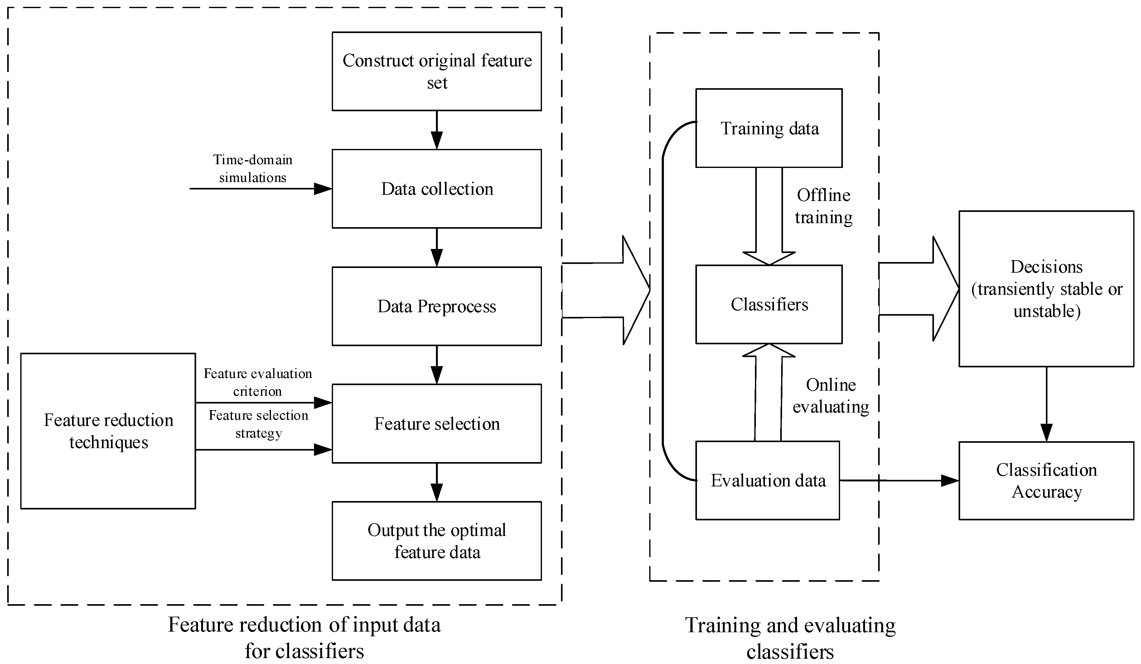
2. Construction Principles of the Initial Input Features for Transient Stability Assessment

The construction of initial input features is foundation of machine learning-based TSA methods, which has a significant impact on the precision of classifiers. The initial features can be established from different perspectives. For example, according to time order, features at fault-free, fault-occurring and fault-clearing time can be selected. By collecting feature data at different running statuses, the impact of fault on the system can be reflected more sufficiently and accurately. In terms of variation of feature size, there are two kinds of features, including system-level features and single-machine features [19,27]. The system-level features are combination indices which are computed by state data of multiple components in system. Thus, the feature dimension will not change with the variation of system size. The single-machine features are state data of single component in system, such as the rotor angle, rotor angular velocity and rotor kinetic energy of each generator. The larger the size of system is, the greater the number of single-machine features is. From the view of sample learning, the features may be closely or indirectly related to classification.

A reasonable initial feature set should follow the system principle, mainstream principle and real-time principle [19,26,27]. System principle refers to that the initial feature set should be system-level to keep its size fixed while the system scale increases. In such cases, the initial features are combination indices of different state data in power system. The mainstream principle means that there should exist high relevance between the selected features and transient stability of power system. The real-time principle requires that the selected features can fully reflect the running state of power system after a fault occurs. Based on the existing researches [11,12,13,14,15,16,17,18,19,25,26,27], 32 features following the above principles are chosen to form the initial feature set after a great deal of time domain simulations, where t₀ , t₁ and t₂ represent the fault-free time, fault-occurring time and fault-clearing time respectively. The details are shown in

Table 1. The initial feature set.

Feature	Feature Description
1	Mean value of all the mechanical power at t0
2	Total energy adjustment of system
3	Maximum value of active power impact on generator at t1
4	Minimum value of active power impact on generator at t1
5	Mean value of generator accelerating power at t1
6	Rotor angle relative to center of inertia of generator with the maximum acceleration at t1
7	Generator rotor angle with the maximum difference relative to center of inertia at t1
8	Mean value of all generator angular acceleration at t1
9	Generator angular acceleration with the maximum difference relative to center of inertia at t1
10	Variance of all generator angular acceleration at t1
11	Variance of all generator accelerating power at t1
12	Mean value of all generator accelerating power at t2
13	Maximum generator rotor kinetic energy at t2
14	Mean value of generator rotor kinetic energy at t2
15	Rotor kinetic energy of generator with the maximum angular acceleration at t2
16	Active power impact on system at t2
17	Rotor angle relative to center of inertia of generator with the maximum rotor kinetic energy at t2
18	Difference of generator rotor angle relative to center of inertia at t1 and t2
19	Generator rotor angle with the maximum difference relative to center of inertia at t2
20	Difference of generator rotor angular velocity relative to center of inertia at t1 and t2
21	Generator rotor angular velocity with the maximum difference relative to center of inertia at t2
22	Difference of maximum and minimum generator rotor angular velocity at t2
23	Difference of generator rotor acceleration relative to center of inertia at t1 and t2
24	Generator rotor acceleration with the maximum difference relative to center of inertia at t2
25	Difference of maximum and minimum generator rotor acceleration at t2
26	Difference of maximum and minimum generator rotor kinetic energy at t2
27	Difference of maximum and minimum variation of generator rotor kinetic energy at t2
28	Sum of generator active power at t2
29	Difference of maximum and minimum generator rotor angle at t2
30	Variance of all generator accelerating power at t2
31	Mean value of all generator rotor angular velocity at t2
32	Mean value of all the mechanical power at t2

.

From Table 1, it’s easy to see that all initial features are independent of system size, which reflect the system principle. From the perspective of real-time principle, features at three different running statuses of system are considered, where features 1,2 are selected to reflect the impact of operation status on system. Features 3–11 reflect the break of power balance at the moment when fault happens. Features 12–32 reflect the impact of unbalanced energy during the fault on power balance. From the point of mainstream principle, features correlated with rotor statuses and operation conditions may reveal the stable tendency and operation status of system. More specially, features 6,7,17–19,29 are related to rotor angle, which can reflect the synchronization conditions between generators. Features 5,8–15,20–27,30,31 are correlated with rotor speed and acceleration, which can reflect the impact of disturbance on rotor movement. Features 1–4,16,28,32 are associated with operation conditions, which reflect the impact of fault on power balance.

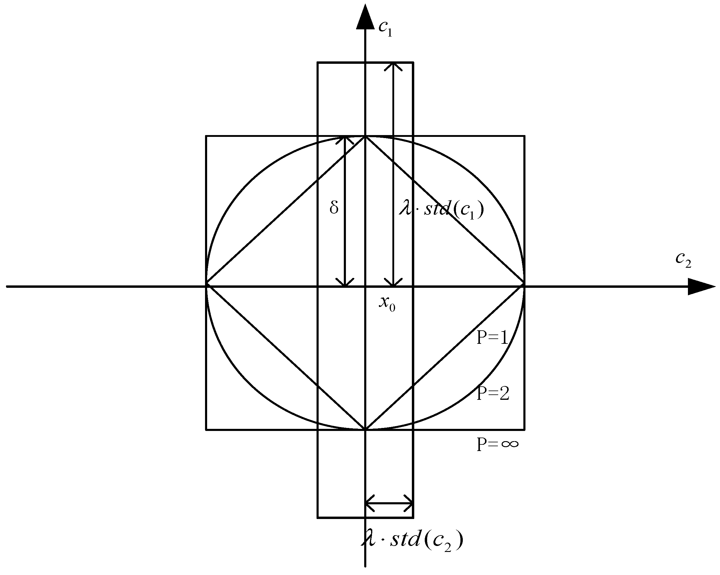
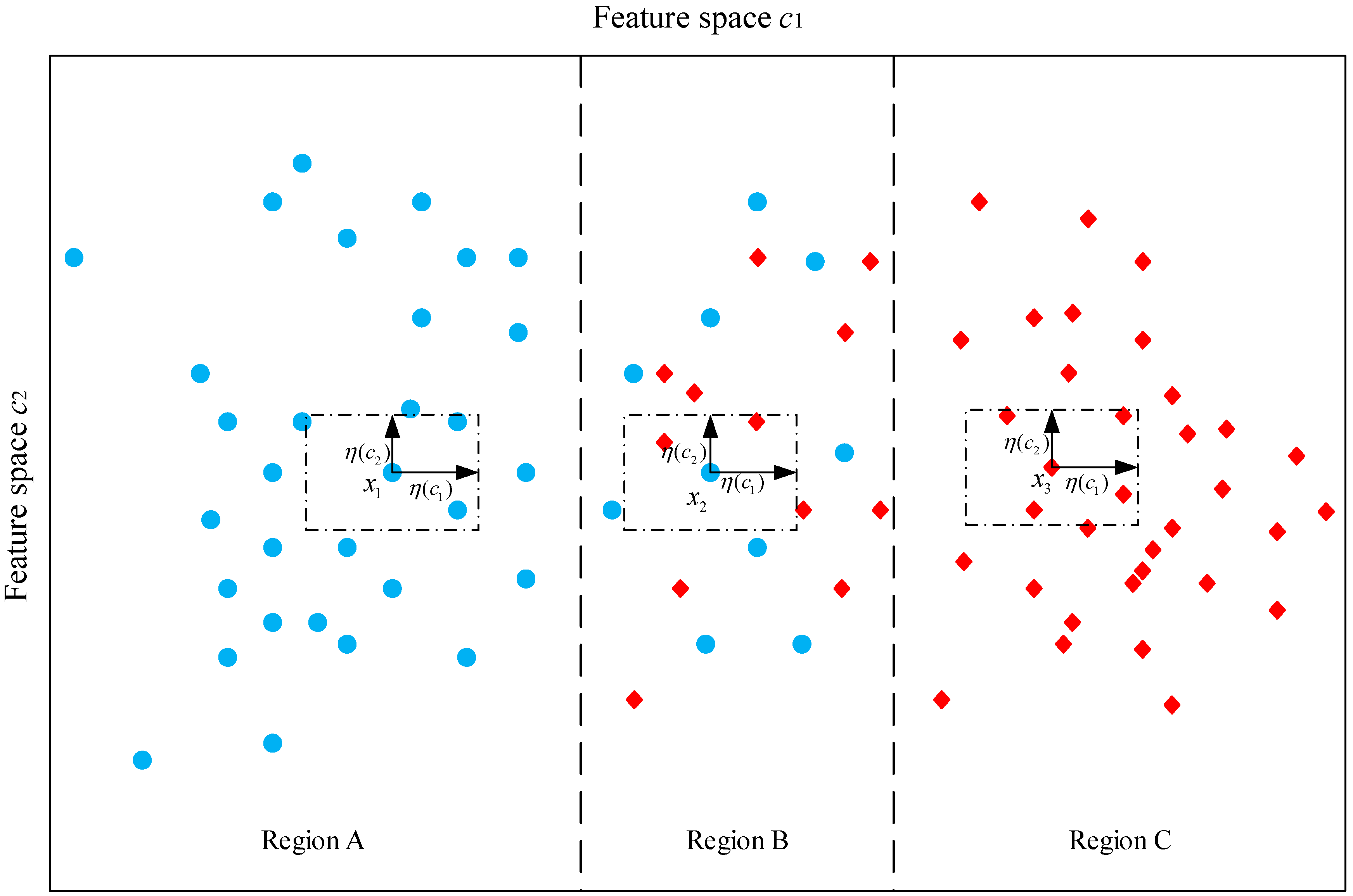
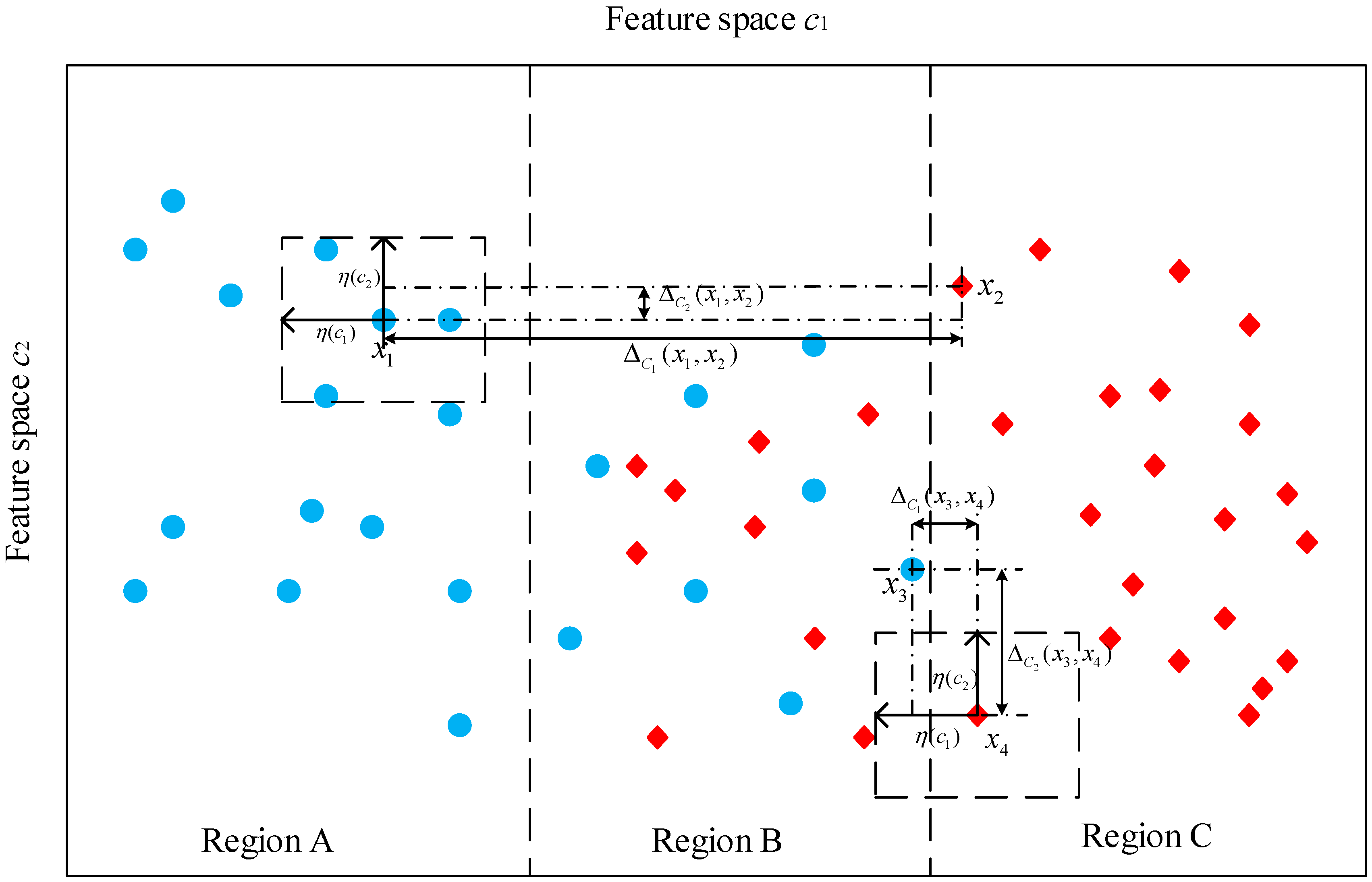
3. Fundamentals on Neighborhood Rough Set

From the view of NRS, a classification task is treated as an information system $IS=\langle U,C,D\rangle$, where $U$ is a finite set of sample data, $C=\{c_1,c_2,\dots ,c_n\}$ is the set of conditional attributes (features) and $D$ is the decision attribute (transient stability state). $IND(D)=\{(x,y)\in U\times U|f(x,D)=f(y,D)\}$ is used here to denote the equivalence relation induced by $D$ and the equivalence class of $IND(D)$ including $x_i$ is denoted by $[x_i]{}_D$, Moreover, $IS$ is also referred to as a decision system.

Definition 1

[29]. Let $IS=\langle U,C,D\rangle$ be an information system, where $U=\{x_1,x_2,\dots ,x_m\}$ is the set of samples, $C=\{c_1,c_2,\dots ,c_n\}$ is the set of conditional attributes, $B\subseteq C$ and $D$ is the decision attribute. Then, the neighborhood of $x_i(i=1,2,\dots ,m)$ in $B$ is defined as follows:

$${\eta }_B(x_i)=\left\{x_j|x_j\in U,{\Delta }_B(x_i,x_j)\le \eta \right\}$$

(1)

where ${\eta }_B(x_i)$ denotes the neighborhood of $x_i$, $\eta$ is the threshold ranges in [0, 1] which controls the size of neighborhood, ${\Delta }_B$ is a distance function, usually defined by the following P-norm.

$${\Delta }_B(x_i,x_j)={\left({\displaystyle {\sum }_{k=1}^N\left|f(x_i,c_k)-f{(x_j,c_k)}^p\right|}\right)}^{1/p}$$

(2)

It’s noted that the neighborhood defined in Equation (1) is uniform, which ignores the difference of data distribution. However, the distributions of data in different attributes are usually quite different in practice. It’s evident that the attribute where data is more scattered carries greater weight in Equation (1). In other words, the higher the standard deviation of the deleted feature is, the more samples may be added in the neighborhoods. In [30], different neighborhood thresholds are used for different types of features to solve the heterogeneous feature selection problem. Inspired by this, in this paper, different neighborhood thresholds are employed according to the data distribution. Based on the above analysis, the definition of neighborhood in NRS is rewritten as follows.

Definition 2.

Let $IS=\langle U,C,D\rangle$ be an information system, where $U=\{x_1,x_2,\dots ,x_m\}$ is the set of samples, $C=\{c_1,c_2,\dots ,c_n\}$ is the set of conditional attributes, $B\subseteq C$ and $D$ is the decision attribute. Then, the neighborhood of $x_i(i=1,2,\dots ,m)$ in $B$ is defined as follows:

$${\eta }_B(x_i)=\left\{x_j\in U|{\wedge }_{k=1}^n\left|f(x_i,c_k)-f(x_j,c_k)\right|\le \eta (k)\right\}$$

(3)

where $\eta (k)=\lambda \cdot std(c_k),\lambda \in [0,1]$, $std(c_k)$ denotes the standard deviation of data in feature space $c_k$ and $\lambda$ is a control parameter ranges in [0, 1], which determines the size of neighborhood in the specified feature space. Take a 2-dimensional feature space as example, the neighborhoods defined by Equations (2) and (3) are shown in Figure 2. It can be seen that as to Equation (3), the higher the standard deviation, the larger the neighborhood is; Thus, when we delete one feature, the number of added samples in neighborhoods would not be influenced by its data distribution. In such case, the information system is also called a neighborhood information system $NIS=\langle U,C,D,\eta \rangle$.

Differing from the equivalent relation of rough set, the similarity relation of sample pairs induced by the neighborhood granules ${\eta }_B(x_i)$ and feature space $B$ is referred to as a neighborhood similarity relation, denoted by $N_B=\{\langle (x_i,x_j),r_{ij}\rangle |(x_i,x_j)\in (U\times U)\}$, where:

$$r_{ij}=\{\begin{array}{ll}1,& {\wedge }_{k=1}^n\left|f(x_i,c_k)-f(x_j,c_k)\right|\le \eta (k)\\ 0,& otherwise\end{array}$$

(4)

$N_B$ reflects neighborhood information of each sample. $x_j$ belongs to neighborhood of $x_i$ and we say that $x_j$ is similar to $x_i$, if $r_{ij}=1$. It’s evident that $N_B$ is symmetric and reflexive.

Definition 3.

[29]. Let $NIS=\langle U,C,D,\eta \rangle$ be a neighborhood information system, where $U=\{x_1,x_2,\dots ,x_m\}$ is the set of samples, $C=\{c_1,c_2,\dots ,c_n\}$ is the set of conditional attributes, $B\subseteq C$ and $D$ is the decision attribute. $d_1,d_2,\dots ,d_N$ are equivalence classes obtained by $D$. Then, the upper and lower rough approximations of $D$ with respect to $B$ is defined as follows:

$$\underset{\_}{N_B}D={\cup }_{i=1}^N\underset{\_}{N_B}{d}_i;\overline{N_B}D={\cup }_{i=1}^N\overline{N_B}{d}_i$$

(5)

where

$$\underset{\_}{N_B}{d}_i=\left\{x_j\right|{\eta }_B(x_j)\subseteq d_i,x_j\in U\},\overline{N_B}{d}_i=\{x_j|{\eta }_B(x_j)\cap d_i\ne \varnothing ,x_j\in U\}$$

The lower rough approximation is also referred to as the positive region of decision attribute, denoted by $PO{S}_B(D)$, which reflects the capability of conditional attributes to approximate the decisions. By Definition 3, we could see that the neighborhoods of samples in positive region can be certainly divided into the same class. Namely, all samples similar to the one in positive region have the same class label. Thus, samples in the positive region can be definitely classified into one decision class, which are beneficial to the classification. Furthermore, the complementary set of lower approximation in upper approximation is called the boundary region, which reflects the inconsistency between conditional attributes (features) and decision class. Unlike the positive region, the neighborhoods in boundary region are inconsistent on the decision labels, which means that the similar samples may belong to different classes. Thus, it’s easy to misclassify the samples in boundary region. From the above analysis, we can find that by dividing the input space into positive region and boundary region, the separability of the feature space is distinct, which can well reflect the classification ability of input data. Thus, we adopt the positive region to act as the evaluation index of feature space. To better illustrate the rationale of the above definitions, we take example of two-pattern classification in a two-dimensional feature space, namely, $C=\{c_1,c_2\}$. The samples are divided into two classes $d_1$ and $d_2$, where samples in $d_1$ are labeled by red rhombus and samples in $d_2$ are labeled by blue dot. The demonstration of positive and boundary region is shown in Figure 3. Suppose that the neighborhoods of samples $x_1,x_2,x_3$ computed by Equation (3) are the rectangular regions shown in Figure 3. Since $\eta (x_1)\subseteq d_1$ and $\eta (x_3)\subseteq d_2$, we can obtain that $x_1,x_3\subseteq PO{S}_C(D)$. Similarly, since $\eta (x_2)\not\subset d_1$ and $\eta (x_2)\not\subset d_2$, we can conclude that $x_2$ belongs to the boundary region. In general, the positive region includes region A and region C, while the region B belongs to the boundary region.

Theorem 1.

Let $NIS=\langle U,C,D,\eta \rangle$ be a neighborhood information system, where $U=\{x_1,x_2,\dots ,x_m\}$ is the set of samples, $B_1\subseteq C,B_2\subseteq B_1$, $D$ is the decision attribute and $d_1,d_2,\dots ,d_N$ are equivalence classes obtained by $D$, then we have:

$$\underset{\_}{N_{B_2}}D\subseteq \underset{\_}{N_{B_1}}D;\overline{N_{B_1}}D\subseteq \overline{N_{B_2}}D$$

Proof. 

Suppose $B_2=\{c_1,c_2,\dots ,c_k\}$ and $B_1=\{c_1,c_2,\dots ,c_k,c_{k+1},\dots ,c_{k+n}\}$. According to Definition 2, we can obtain that ${\eta }_{B_1}(x_i)=\left\{x_j\in U|({\wedge }_{l=1}^k\left|f(x_i,c_l)-f(x_j,c_l)\right|\le \eta (l))\wedge ({\wedge }_{l=k+1}^{k+n}\left|f(x_i,c_l)-f(x_j,c_l)\right|\le \eta (l))\right\}$ and ${\eta }_{B_2}(x_i)=\left\{x_j\in U|{\wedge }_{l=1}^k\left|f(x_i,c_l)-f(x_j,c_l)\right|\le \eta (l)\right\}$. Hence, there exists ${\eta }_{B_1}(x_i)\subseteq {\eta }_{B_2}(x_i)$. By Definition 3, we have $\underset{\_}{N_{B_2}}D\subseteq \underset{\_}{N_{B_1}}D$ and $\overline{N_{B_1}}\subseteq \overline{N_{B_2}}$. □

By Theorem 1, we can see that deleting features will cause the expansion of neighborhoods and the neighborhood granules will coarsen. Moreover, with the expansion of neighborhood, the decisions of samples in neighborhood may be inconsistent, which leads to the diminution of positive region. This implies that the increase of features can enlarge the positive region and strengthen the classification ability of input data.

Definition 4.

Let $NIS=\langle U,C,D,\eta \rangle$ be a neighborhood information system, where $U=\{x_1,x_2,\dots ,x_m\}$ is the set of samples, $C=\{c_1,c_2,\dots ,c_n\}$ is the set of conditional attributes, $B\subseteq C,a\in B$ and $D$ is the decision attribute. $d_1,d_2,\dots ,d_N$ are equivalence classes obtained by $D$. Then, the dependency of $D$ to $B$ is defined as follows:

$${\gamma }_B(D)=Card(PO{S}_B(D))/Card(U)$$

(6)

The significance of $a$ to $B$ is defined as:

$$si{g}_B(a)={\gamma }_B(D)-{\gamma }_{B-\left\{a\right\}}(D)$$

(7)

where $Card(X)$ is the cardinality of a set $X$. The dependency ${\gamma }_B(D)$ indicates the proportion that the samples characterized by the feature set $B$ necessarily belong to their classes. Namely, ${\gamma }_B(D)$ reflects the ability of $B$ to approximate the decision. In special, the information system is called consistent if ${\gamma }_B(D)=1$. In this case, all samples certainly belong to their classes. We say that $a_i$ is indispensable in $B$, if $si{g}_B(a_i)>0$ , otherwise, $a_i$ is dispensable in $B$. The collection of all indispensable attributes or features in $B$ is called core set of $B$ to $D$, denoted by $COR{E}_D(B)$. By Definitions 3 and 4, we can see that for any $B\subseteq C$, there exist $PO{S}_B(D)\subseteq PO{S}_C(D)$ and ${\gamma }_B(D)\le {\gamma }_C(D)$. $B\subseteq C$ is referred to as a reduction of $C$ to $D$ if ${\gamma }_B(D)={\gamma }_C(D)$ (or equivalently $PO{S}_B(D)=PO{S}_C(D)$) and $\forall B^{\prime }\subseteq B$, there exists ${\gamma }_{B^{\prime }}(D)<{\gamma }_B(D)$. That is, feature reduction is to make the number of features least and keep the positive region invariable.

4. Feature Reduction Using Neighborhood Rough Set and Discernibility Matrix

From the previous discussion in Section 3, we know that the positive region reflects the classification ability of input data. Thus, from the view of NRS, feature reduction is to find a feature subset which contains the least number of features and keeps the same positive region as the original feature set. To discern the conditions whereby a feature subset can keep the same positive region as the original feature set, we defined the discernibility matrix for neighborhood rough set, which is an important method in granular computing [31,32,33]. Based on that, a feature selection strategy by using discernibility matrix is designed to find the feature reduction. To better illustrate it, we first take the neighborhood information system defined in Theorem 1 as an example and illustrate that in what conditions does $B_2$ keep the same positive region as $B_1$.

By Theorem 1, we know that deleting attributes will diminish the positive region of decision attribute. This is caused by the expansion of neighborhoods of samples, which increases the inconsistency of decisions of individuals in neighborhoods. Thus, if we hope that $PO{S}_{B_2}(D)=PO{S}_{B_1}(D)$ holds, neighborhoods induced by $B_2$ should keep consistent with neighborhoods induced by $B_1$. In other words, if $B_1$ can separate from $x_i\in \underset{\_}{N_{B_1}}{d}_l$ and $x_j\notin \underset{\_}{N_{B_1}}{d}_l$, then so can $B_2$. Hence, for any $x_i\in PO{S}_{B_1}(D)$, neighborhood of $x_i$ induced by $B_2$ should not contain any individual with different decision classes. According to Definition 2, we can obtain that for any individual $x_j$ possessing different decision classes, there should exist $c_{l^{\prime }}$ satisfying $\left|f(x_i,c_{l^{\prime }})-f(x_j,c_{l^{\prime }})\right|>\eta (l^{\prime })$ to ensure $x_j\notin {\eta }_{B_1}(x_i)$, where $c_{l^{\prime }}\in B_2$. To better demonstrate the rationale, we still take the two-pattern classification problem in Section 3 as an example and present it in Figure 4. As we can see, samples $x_1$ and $x_2$ belong to the positive region since their neighborhoods have consistent class labels. However, if we delete feature $c_1$, these two samples will be no longer belong to the positive region, since they are similar in terms of feature $c_2$, while they have different class labels. Thus, if we want to keep the positive region invariable, $c_1$ is needed to distinguish samples $x_1$ and $x_2$. Similarly, feature $c_2$ is needed to distinguish samples $x_3$ and $x_4$, otherwise, $x_3$ will belong to the neighborhood of $x_4$ in terms of feature $c_1$ and the positive region will diminish. Namely, as to the discussed problem in Figure 4, both features $c_1$ and $c_2$ should be reserved to maintain the classification ability. Based on the above analysis, we define the discernibility matrix for neighborhood rough set as follows.

Definition 5.

Let $NIS=\langle U,C,D,\eta \rangle$ be a neighborhood information system, where $U=\{x_1,x_2,\dots ,x_m\}$ is the set of samples, $C=\{c_1,c_2,\dots ,c_n\}$ is the set of features and $D$ is the decision attribute. $d_1,d_2,\dots ,d_N$ are equivalence classes obtained by $D$. Then, the discernibility matrix of NIS is denoted by a $m\times m$ matrix $M_D(C)={(m_{ij})}_{m\times m}$ as follows:

$$m_{ij}=\{\begin{array}{l}\left\{c_k\in C|\left|f(x_i,c_k)-f(x_j,c_k)\right|>\eta (k)\wedge con(x_i,x_j)\right\}\\ \varnothing ,\hspace{1em}otherwise\end{array}$$

(8)

where $con(x_i,x_j)$ satisfies $x_i,x_j\in PO{S}_C(D)\wedge f(x_i,D)\ne f(x_j,D),x_i\in PO{S}_C(D)\wedge x_j\notin PO{S}_C(D)$ or $x_i\notin PO{S}_C(D)\wedge x_J\in PO{S}_C(D)$. Samples $(x_i,x_j)$ satisfying $con(x_i,x_j)$ have different decision labels and $m_{ij}$ is the collection of features, where distance between $x_i$ and $x_j$ exceeds the corresponding neighborhood threshold. This implies that if all relevant features in $m_{ij}$ are deleted, $x_i$ and $x_j$ will not be distinguished and both the samples will be contained in the boundary region. In other words, at least one feature in $m_{ij}$ should be reserved to distinguish $x_i$ and $x_j$. By Equation (8), we can see that the discernibility matrix is symmetric and $m_{ii}=\varnothing$. Thus, we can only compute the upper or lower triangular matrix in practice.

Theorem 2.

Let $NIS=\langle U,C,D,\eta \rangle$ be a neighborhood information system, where $U=\{x_1,x_2,\dots ,x_m\}$ is the set of samples, $C=\{c_1,c_2,\dots ,c_n\}$ is the set of features and $D$ is the decision attribute. $M_D(C)={(m_{ij})}_{m\times m}$ is the discernibility matrix defined in Definition 5, then there exists:

$$COR{E}_D(B)=\left\{c_l|m_{ij}=\{c_l\}\right\}$$

(9)

Moreover, if $B\subseteq C$ is a reduction of $C$ to $D$, then for any $m_{ij}\ne \varnothing$, there exists $B\cap m_{ij}\ne \varnothing$.

Proof. 

(1) According to Definition 4, if $c_l\in COR{E}_D(B)$, there exists $si{g}_C(c_l)={\gamma }_C(D)-{\gamma }_{C-\left\{c_l\right\}}(D)>0$. $\iff$ $PO{S}_C(D)\ne PO{S}_{C-\left\{c_l\right\}}(D)$ $\iff$ There exists $x_i\in U$, such that ${\eta }_C(x_i)\subseteq {[x_i]}_D$ and ${\eta }_{C-\left\{c_l\right\}}(x_i)\not\subset {[x_i]}_D$ $\iff$ There exists $x_j\notin {[x_i]}_D$, such that $\left|f(x_i,c_k)-f(x_j,c_k)\right|\le \eta (k)$ $(k=1,2,\dots ,l-1,l+1,\dots ,n)$ and $\left|f(x_i,c_l)-f(x_j,c_l)\right|>\eta (l)$. $\iff$ $M_D(C)(i,j)\cap M_D(C-\{c_l\})(i,j)=c_l$ and $M_D(C-\{c_l\})(i,j)=\varnothing$ $\iff$ $M_D(C)(i,j)=\left\{c_l\right\}$ $\iff$ $m_{ij}=\left\{c_l\right\}$.

(2) $B$ is a reduction of $C$ to $D$ $\iff$ for any $x_i\in PO{S}_C(D)$ satisfying ${\eta }_C(x_i)\subseteq {[x_i]}_D$, there exists ${\eta }_B(x_i)\subseteq {[x_i]}_D$ $\iff$ For any $x_j\notin {\eta }_B(x_i)$, there exist $x_j\notin {\eta }_C(x_i)$. $\iff$ There exists $c_l\in B$ such that $|f(x_i,c_l)-f(x_j,c_l)|>\eta (l)$ $\iff$ According to Definition 5, we can obtain that $m_{ij}\ne \varnothing$ and $c_l\in m_{ij}$ $\iff$ $B\cap m_{ij}\ne \varnothing$. □

From Theorem 2, we can see that features in the core set are used to distinguish a few specific samples and the core set could be empty. Features in reduction can distinguish all sample pairs $(x_i,x_j)$ satisfying $con(x_i,x_j)$, which means that a reduction has the same separability as the original feature space. The remaining features are eliminated since the sample pairs which can be distinguished by them can also be distinguished by features in reduction. From the above analysis, we can add features into the reduction set one by one until the intersection of reduction set and each nonempty unit in discernibility matrix is nonempty. However, this method is inefficient and the obtained reduction set is usually redundant since there isn’t any effective guideline. To find the most important feature in each round, we introduce the following definition. Based on that, we design a feature selection strategy to find the optimal feature set.

Definition 6.

Let $NIS=\langle U,C,D,\eta \rangle$ be a neighborhood information system, where $U=\{x_1,x_2,\dots ,x_m\}$ is the set of samples, $C=\{c_1,c_2,\dots ,c_n\}$ is the set of features and $D$ is the decision attribute. $M_D(C)={(m_{ij})}_{m\times m}$ is the discernibility matrix of NIS, then the discernibility set of $C$ with respect to $M_D(C)$ is defined as $DIS(C)=\left\{m_{ij}\right|m_{ij}\ne \varnothing \}$. The discernibility set of $c_l$ with respect to $M_D(C)$ is defined as $DIS(\{c_l\})=\left\{m_{ij}\right|m_{ij}\ne \varnothing {,}_{}{c}_l\in m_{ij}\}$. Obviously, there exists $DIS(C)={\cup }_{c_l\in C}DIS(\{c_l\})$. The importance of $c_l$ to $M_D(C)$ is defined as:

$$IMP(c_l)=Card(DIS(\left\{c_l\right\}))/Card(DIS(C))$$

(10)

The importance of $c_l$ reflects that the capacity of $c_l$ to distinguish sample pairs $(x_i,x_j)$ satisfying $con(x_i,x_j)$. The higher the importance of $c_l$ is, the greater the ability of $c_l$ is to approximate the decision. To find the feature reduction, we first initialize the reduction set as an empty set and keep adding features into the reduction set one after another until it can distinguish all the sample pairs with nonempty units in $M_D(C)$, where the added feature in each round maximizes the increment of importance of current reduction set. Based on the above analysis, we design a feature selection strategy based on NRS and discernibility matrix to compute the optimal feature reduction, the Algorithm 1 is as follow.

Algorithm 1: Feature Selection Strategy Based on NRS and Discernibility Matrix

Input: Neighborhood information system $NIS=\langle U,C,D,\eta \rangle$, where $U=\{x_1,x_2,\dots ,x_m\}$ is the set of samples, $C=\{c_1,c_2,\dots ,c_n\}$ is the set of features, $D$ is the decision attribute which divides samples into several equivalence classes $\{d_1,d_2,\dots ,d_N\}$. $CORE=\varnothing$, $RED=\varnothing$.

Output: reduction set $RED$

Step 1: Normalize the data by 0-1 normalization method to decrease the influence caused by difference of units of measures.

Step 2: Compute the discernibility matrix $M_D(C)$ of NIS and the discernibility set $DIS(C)$ of $C$ to $M_D(C)$. Choose the nonempty units $m_i$ in $DIS(C)$ with single feature, and put them into core set $CORE$.

Step 3: For each unit $m_i$ in $DIS(C)$, if the intersection of $m_i$ and $CORE$ is not empty, delete the unit from $DIS(C)$.

Step 4: Put the features in core set into reduction set, namely, $RED=CORE$.

Step 5: If $DIS(C)=\varnothing$, then go to Step 7, otherwise, go to Step 6.

Step 6: For each feature $c_l\notin RED$, compute the discernibility set $DIS(\{c_l\})$ and importance $IMP(c_l)$ of $c_l$ to $M_D(C)$. Find the maximum $IMP(c_l)$ and the corresponding feature $c_l$. Put $c_l$ into reduction set $RED$ and delete units which includes $c_l$ from $DIS(C)$. Then go to Step 5.

Step 7: Output the reduction set $RED$.

The computation complexity of constructing discernibility matrix is equal to $O(|U{|}^2\times n)$ and the computation complexity of computing core set and reduction is $O(|U{|}^2\times n)$. Thus, the overall computation complexity of the proposed algorithm is $O(|U{|}^2\times n)$. In practice, it can be found that most of sample pairs can be distinguished by the feature with maximum importance. Since each time we add a new feature into reduction set, the size of $DIS(C)$ will be reduced. Thus, the computation times will decrease after each round, especially at the start of search.

5. Illustrative Example

In this section, the proposed method is applied to the New England 10 generator 39 bus system and Australian simplified 14 generators system to illustrate its effectiveness. Moreover, comparative experiments are also provided to analyze its performance.

5.1. New England 10 Generator 39 Bus System

The New England 10 generator 39 bus system (NES39) [34] is a well-known test system for the study of transient stability and dynamic security analysis. This benchmark includes 10 generators, 39 buses, 19 loads and 46 transmissions, where the generator 1 represents an interconnected power system in Canada.

According to features listed in Table 1, we first generate the initial sample space after a large amount of offline time domain simulations. 10 different basic load conditions (80%, 85%, …, 125%) are considered and the generator outputs are changed accordingly to ensure the power balance of system. Three-phase short-circuit fault on each bus is set as the contingency, which is happened at 0.1 s and cleared at 0.2 s, 0.25 s, 0.3 s or 0.35 s, respectively and there isn’t topology change from the fault. The simulation time is set as 3s. We randomly choose 15 different fault locations at each load level and 600 samples are generated, with 315 stable samples and 285 unstable samples. Seventy percent of samples are used to train the classifiers, and the rest are used to test. The constant impedance load and 4th order generator model are considered in this system. The IEEE type DC1 is used as the excitation system model. The decision system consists of feature data and the corresponding transient stability state. The maximum difference of any two generators at the stop time of simulation is used to judge if the system is transiently stable or not. If it doesn’t exceed ${180}^{\circ }$, the system is transiently stable and we mark the decision label of corresponding sample data with “1”; otherwise, the system is transiently unstable and we mark the decision label of sample data with “0”. The above experiments are all carried out in MATLAB/Simulink (2013b, MathWorks, Natick, MA, USA).

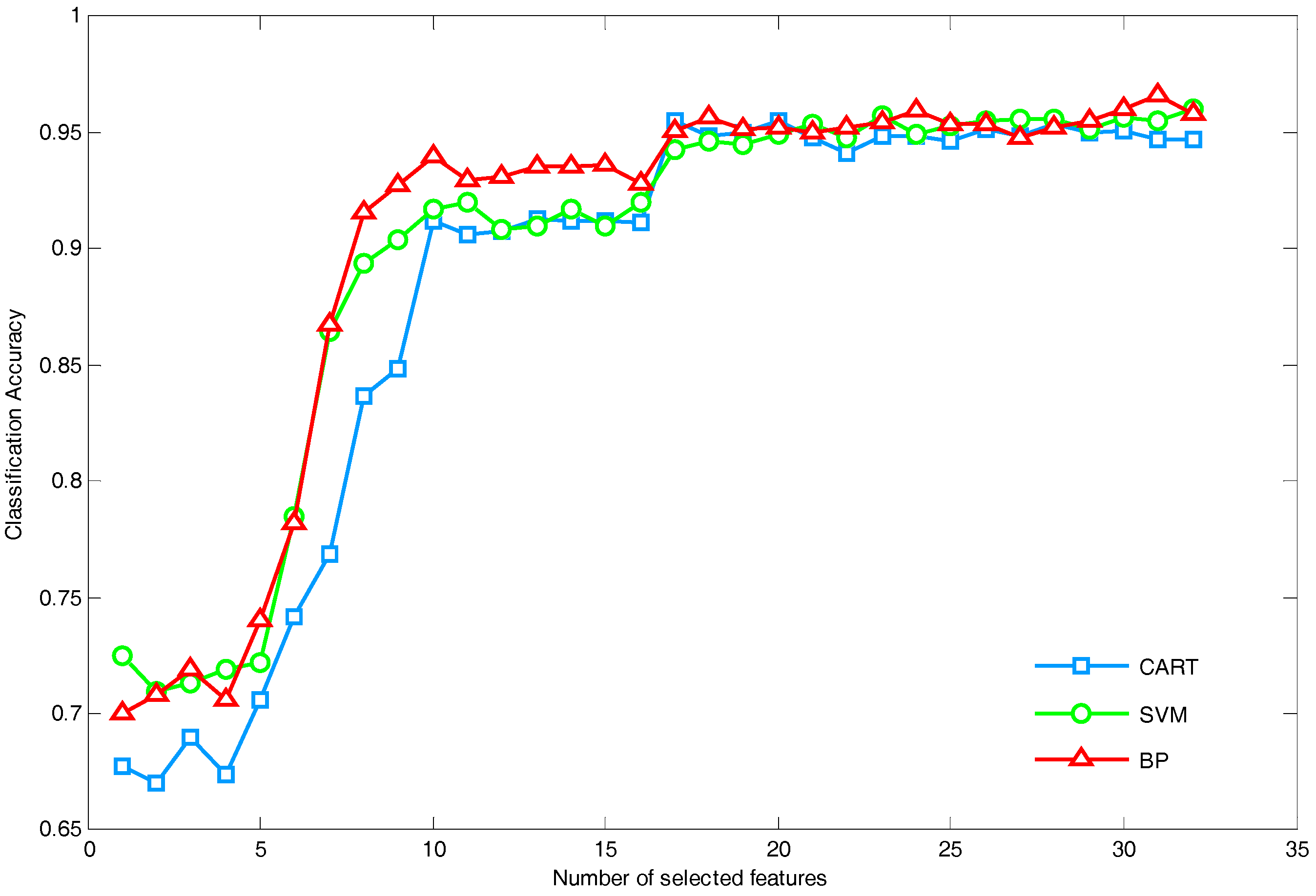
5.1.1. Performance Analysis of Feature Selection Strategy

By using the positive region of NRS theory as the evaluation index, different feature selection strategies could be used to search the optimal feature set. To illustrate the effectiveness and superiority of our proposed feature selection strategy, in this subsection, we first discuss the performance of the proposed feature selection strategy by some comparative analysis. To avoid the occasionality, three representative classifiers including back propagation neural network (BP), radial basis function based support vector machine (RBF-SVM) and classification and regression tree (CART) are selected to evaluate classification performance of the reduction set. The least-squares method is used to find the separating hyperplane and the kernel parameter is set as 2 in RBF-SVM. As to BP, we adopt two hidden layers and the L-M algorithm as training function. The classification accuracies are tested 100 times and the statistics are utilized to evaluate the characteristic of selected features. To explore the correlations between number of features and classification performance, we first analyze the ranking based feature selection strategy (Ranking for short) [24]. By comparing the significance (see Definition 4) of single features, features with greater significance are added one after another. The classification accuracies with different number of selected features are presented in Figure 5. It can be seen that the classification accuracy increases distinctly at the start of the screening process. After adding 17 features, the classification accuracy doesn’t visibly increase and maintain in 0.95 approximately. This indicates that there is redundant information in the original feature space, thus, it’s necessary to further reduce the original features.

Two other widely used feature selection strategies for NRS including the forward heuristic search (Forward for short) and the backward heuristic search (Backward for short) [30] are also employed here to make comparisons. The results are shown in

Table 2. Performance comparison of different feature selection strategies (NES39).

Feature Selection Strategy	Selected Features in Reduction	Accuracy (%) CART	Accuracy (%) RBF-SVM	Accuracy (%) BP	Computation Time
DM	17,1,10,7,3,2	95.33 ± 1.84	95.80 ± 1.76	95.75 ± 1.69	162.37 s
Forward	17,5,1,24,3,6	94.10 ± 2.03	95.23 ± 2.03	94.29 ± 1.63	224.55 s
Backward	9,22,26,29,31,32	96.03 ± 2.17	95.60 ± 1.92	95.07 ± 1.86	340.28 s

, where our proposed feature selection strategy is denoted by DM for short. The orders of selected features in Table 2 are arranged by the orders of features added by the corresponding algorithm.

As shown in Table 2, we can see that all the above strategies finally select six features. However, the feature reductions obtained by these three strategies are quite different. For instance, as to DM, features 17,1,10,7,3,2 are selected while features 17,5,1,24,3,6 are chosen by Forward. There are three features identical. As to Backward, the obtained reduction set includes features 9,22,26,29,31,32, which are completely different from the selected features obtained by DM or Forward. The differences mainly arose from different search strategies. From the view of classification performance, we could find that all the feature reductions selected by the above strategies have similar classification abilities with the original feature set. However, the features selected by DM have more stable test results, which are more ideal. In terms of computation time, it is easy to find that DM has spent less computation time. The underlying reason is that the maximum computation complexity of DM is $O(|U{|}^2\times n)$ while the maximum computation complexity of Forward and Backward is $O(|U{|}^2\times n^2)$, where $\left|U\right|$ represents the number of samples and $n$ represents the number of features. Thus, the proposed discernibility matrix based feature selection strategy is more efficient to find the optimal feature reduction.

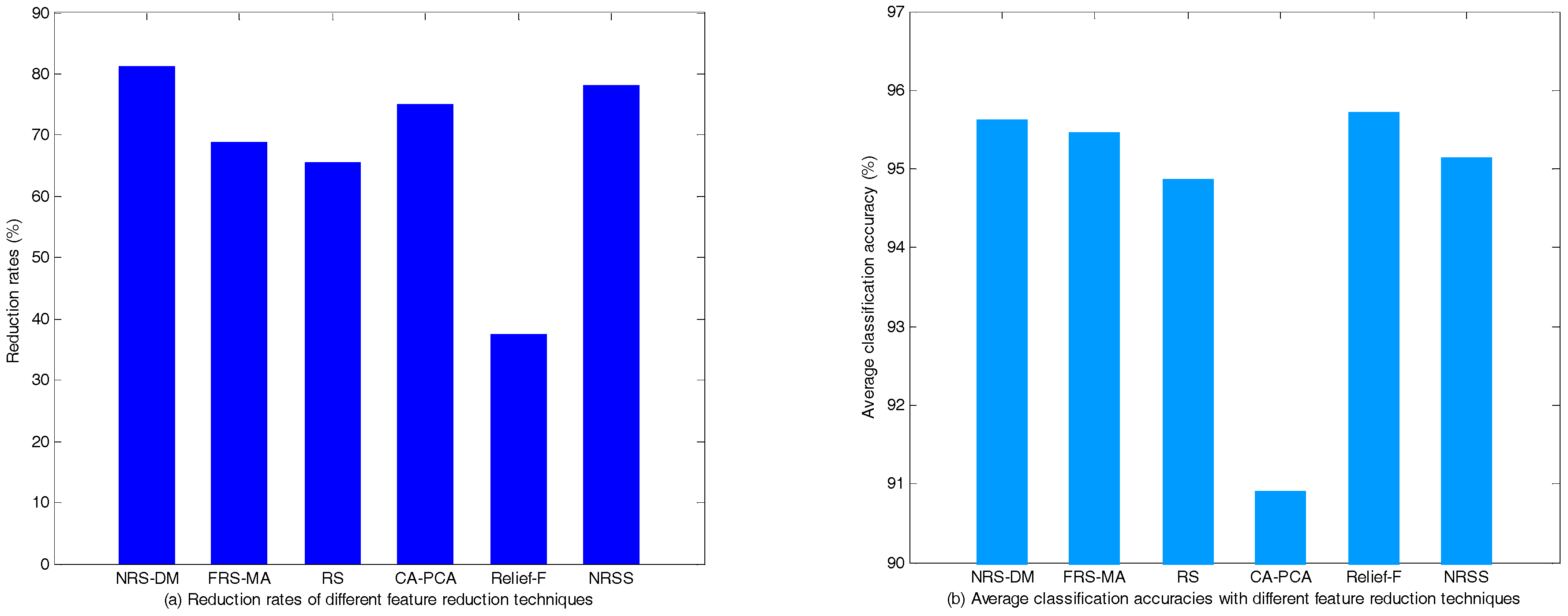
5.1.2. Performance Comparison of Different Feature Reduction Methods

It’s noteworthy that a feature reduction method consists of both a feature evaluation index and the feature selection strategy. In order to analyze the performance of our proposed feature reduction method, we further compare our method with several existing feature reduction methods of TSA, which include the Pawlak rough-set-based method (RS for short) [25,26], the kernelized fuzzy rough set and memetic algorithm based method (FRS-MA for short) [27], correlation analysis and principle component analysis based method (CA-PCA for short) [11] and Relief-F [35]. Our proposed feature reduction method is denoted by NRS-DM for short. The above-mentioned methods have different feature evaluation indexes and feature selection strategies. In the meanwhile, we report the reduction performance of NRS with single neighborhood threshold (NRSS for short), where the threshold is set as 0.1 according to the recommended value range of neighborhood threshold in [28]. Some basic configurations are given as follows. The population size and maximum generation are set as 30 and 100 respectively in FRS-MA. The equal frequency discretization is used in RS and the frequency is set as 4. In CA-PCA, if the correlation of each pair of features is greater than 0.95, we delete one of them. Moreover, 95% of variation of feature space is considered in PCA. As to Relief-F, each feature negative correlative with the classification will be deleted. The results are given in

Table 3. Comparison of different feature reduction methods (NES39).

Feature Reduction Method	Selected Optimal Feature Set	Dimension	Accuracy (%) CART	Accuracy (%) RBF-SVM	Accuracy (%) BP
NRS-DM	17,1,10,7,3,2	6	95.33 ± 1.84	95.80 ± 1.76	95.75 ± 1.69
FRS-MA	1,2,4,7,8,14, 17,23,26,31	10	95.08 ± 2.02	95.28 ± 1.71	96.02 ± 1.88
RS	17,2,13,12,21,7, 3,27,25,4,9	11	95.12 ± 1.87	94.25 ± 2.08	95.29 ± 2.08
CA-PCA	* 1,2,3,4,5,6,7,8,9,12,13,17, 19,20,21,24,25,26,27,29,30	8	88.30 ± 2.43	92.12 ± 2.35	92.28 ± 1.95
Relief-F	2,7,8,9,10,13,14,16,17,18, 19,21,22,23,24,25,28,30,31,32	20	95.12 ± 1.78	96.08 ± 1.34	95.96 ± 1.80
NRSS	17,5,32,1,7,6,3	7	95.92 ± 1.78	94.45 ± 1.87	95.04 ± 2.38
The original feature set	--	32	94.75 ± 2.06	95.67 ± 1.63	96.46 ± 1.69

. Figure 6 shows the corresponding reduction rates and average classification accuracies of three classifiers. The orders of selected features in Table 3 are arranged by the orders of features added by the corresponding method. Since the final feature space has changed, in Table 3, we only provide features obtained by CA for CA-PCA (labeled by *).

From Table 3 and Figure 6, we can find that the dimension of features selected by NRS-DM is only one fifth of the original feature set, but the corresponding classification accuracies are similar to or even better than the original feature set. As to FRS-MA and RS, there are 10 and 11 features selected respectively, which are more than NRS-DM. Moreover, their average classification accuracies are lower than NRS-DM. The above differences may result from two aspects. One is the difference of feature selection strategies. As we discussed above, a sound search strategy has a direct impact on the result of feature reduction. Since the randomness of evolutionary algorithm, FRS-MA may be trapped into local optimal. Moreover, the result is susceptible to the control parameters setting. In contrast, NRS-DM is more robust and has a good suitability for feature reduction. The other is the used evaluation index. Since RS is based on the equivalence relation, it can’t directly handle the real-valued data, which means that we need to discretize input data first. As we know, data discretization will inevitably result in information loss. In contrast, the equivalence relation is replaced by the neighborhood similarity relation in NRS-DM, which avoids the influence of discretization. The results of NRSS show that NRS with multiple neighborhood thresholds has better performance than the one with single threshold. As to CA-PCA, we can see that at the first round, 21 features are selected by correlation analysis and the dimension is finally reduced to 8 by PCA at the second round. The final reduction rate is high to 75%, however, the classification performance is not as high as NRS-DM. The underlying reason is that the component with lower variation may include important information closely associated to classification. Moreover, not matter CA or PCA, the decision information is not considered. As to Relief-F, although the selected features has similar classification accuracies to the original feature set, it can’t effectively eliminate the redundancies in feature space. From the above analysis, it can be seen that NRS-DM performs better than the other feature selection methods for TSA problem.

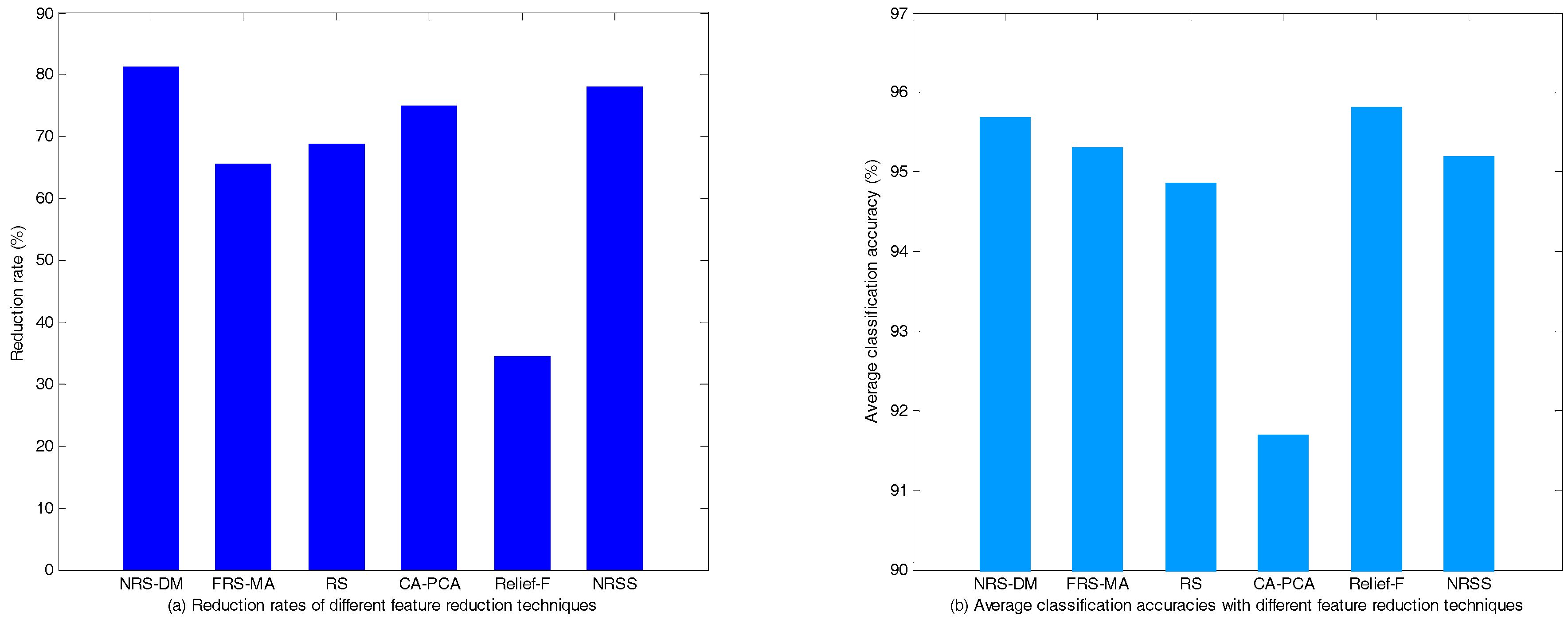
5.1.3. Performance Test in the Condition of N-1 Contingencies

In order to verify the effectiveness of our method in different conditions, in this subsection, the method is tested in the condition of N-1 contingencies, where any one of the transformers or transmission lines is out of the service. A three-phase short-circuit fault on bus is set as the contingency and we randomly choose the fault locations. The load conditions and fault-occurring and fault-clearing time are set in the same way. 600 samples are generated, with 249 stable samples and 351 unstable samples. In the same way, five feature reduction methods mentioned above are applied to make comparisons with the proposed method. The results are presented in Figure 7 and

Table 4. Results in the condition of N-1 contingencies (NES39).

Feature Reduction Method	Selected Optimal Feature Set	Dimension	Accuracy (%) CART	Accuracy (%) RBF-SVM	Accuracy (%) BP
NRS-DM	6,17,29,10,7,2	6	95.44 ± 1.55	95.51 ± 1.31	96.07 ± 1.12
FRS-MA	1,2,3,14,16,17, 19,20,26,31,32	11	95.15 ± 1.46	94.87 ± 1.47	95.87 ± 1.32
RS	13,21,12,9,4,7, 26,8,3,19	10	95.08 ± 1.39	94.93 ± 1.48	94.58 ± 1.45
CA-PCA	* 1,2,3,4,5,6,7,8,9,12,13, 17,19,20,21,25,26,27,29,30	8	89.44 ± 2.06	93.07 ± 1.67	92.58 ± 1.79
Relief-F	2,7,8,9,10,11,13,14,16,17,18, 19,21,22,23,25,28,29,30,31,32	21	95.53 ± 1.37	96.18 ± 1.11	95.73 ± 1.00
NRSS	17,7,1,2,3,6,11	7	95.28 ± 1.22	94.63 ± 1.45	95.69 ± 1.13
The original feature set	--	32	95.43 ± 1.26	95.30 ± 1.19	96.28 ± 1.20

. The results show that the classification accuracy of our method is almost the highest (just little lower than Relief-F). Moreover, compared with other methods, our method owns the highest reduction rate. The results are consistent with the previous conclusions. The underlying reason is that our evaluation index can well reflect the classification ability of input features, it is applicable to different circumstances. Based on that, the proposed feature selection strategy helps us to find the optimal feature set.

5.2. Australian Simplified 14 Generators System

To further illustrate the effectiveness of the proposed method, the Australian simplified 14 generators system (ASS14) [36] is employed in this subsection. The Australian simplified 14 generators system models the southern and eastern Australian power system (refer to [36] for more details). This system includes 14 generators, 59 buses, 29 loads and 114 transmissions. Several power system stabilizers are provided in this system. Moreover, five Static Var Compensators are also included in this system. 10 different basic load conditions (80%, 85%, …, 125%) are considered and the generator outputs are changed accordingly to ensure the power balance of system. Three-phase short-circuit fault on each bus is set as the contingency, which is happened at 0.1 s and cleared at 0.15 s, 0.2 s, 0.25 s or 0.3 s, respectively and there isn’t topology change from the fault. The simulation time is set as 3 s. We randomly choose 30 different fault locations at each load level and 1200 samples are generated, with 727 stable samples and 473 unstable samples. Seventy percent of samples are used to train the classifiers, and the rest are used to test. The constant impedance load and 4th order generator model are considered in this system. The IEEE type AC4A is used as the excitation system model.

5.2.1. Performance Analysis of Feature Selection Strategy

The obtained feature reductions with different feature selection strategies are given in

Table 5. Performance comparison of different feature selection strategies (ASS14).

Feature Selection Strategy	Selected Features in Reduction	Accuracy (%) CART	Accuracy (%) RBF-SVM	Accuracy (%) BP	Computation Time
DM	5,30,13,2,4,8,19,7	96.38 ± 1.45	96.03 ± 1.22	94.02 ± 1.32	209.96 s
Forward	31,32,6,2,29,8,5,13,30	95.25 ± 1.46	95.13 ± 1.43	94.27 ± 1.49	1335.06 s
Backward	5,8,17,22,25,26,29,30,31,32	95.90 ± 1.79	95.94 ± 1.61	94.23 ± 1.48	1447.29 s

. It can be seen that all the three acquired feature reductions have similar classification accuracies, but the number of selected features obtained by DM is less than the other two algorithms. Moreover, it’s noted that the computation time is greatly reduced by DM. This is mainly because that in NRS-DM, most sample pairs can be distinguished by the selected features at the start of algorithm, thus, the dimension of discernibility set will be greatly reduced, which reduces the cycle times. In contrast, each time a new feature is added, the neighborhoods of samples would be recomputed in Forward and Backward. Therefore, as the number of samples increases, the computation time of Forward and Backward will increase exponentially.

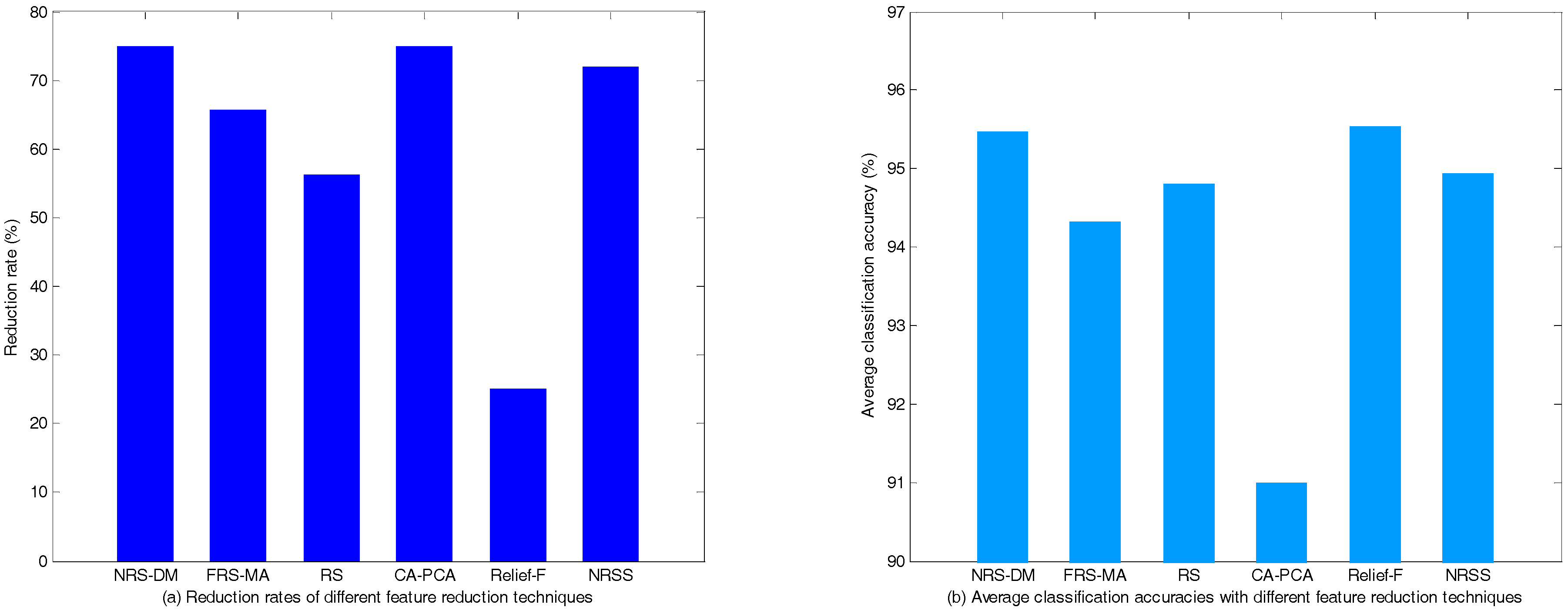
5.2.2. Performance Comparison of Different Feature Reduction Methods

In the same way, five feature reduction methods mentioned above are applied to make comparisons with the proposed method.

Table 6. Comparison of different feature reduction methods (ASS14).

Feature Reduction Method	Selected Optimal Feature Set	Dimension	Accuracy (%) CART	Accuracy (%) RBF-SVM	Accuracy (%) BP
NRS-DM	5,30,13,2,4,8,19,7	8	96.38 ± 1.45	96.03 ± 1.22	94.02 ± 1.32
FRS-MA	2,4,7,13,14,18, 20,21,22,26,31	11	93.79 ± 2.15	95.19 ± 1.66	94.02 ± 1.55
RS	21,16,7,29,2,4,14, 30,10,5,8,17,28,19	14	94.95 ± 1.66	95.04 ± 1.27	94.44 ± 1.10
CA-PCA	* 1,2,3,4,5,6,7,8,9,11,12,13,15, 16,19,20,21,26,27,28,29,30,32	8	90.14 ± 2.15	92.48 ± 1.64	90.38 ± 2.09
Relief-F	2,5,7,8,9,10,11,12,13,14,18,19,20, 21,22,23,24,25,27,28,29,30,31,32	24	95.13 ± 1.50	96.33 ± 1.21	95.15 ± 1.28
NRSS	31,32,1,2,11,5,13,8,30	9	94.90 ± 1.82	95.94 ± 1.24	93.98 ± 1.15
The original feature set	--	32	94.55 ± 1.81	95.63 ± 1.22	94.41 ± 1.62

presents the obtained feature reductions and their classification accuracies. Figure 8 shows the corresponding reduction rates and average classification accuracies of three classifiers. The results show that the feature reductions obtained by NRS-DM and CA-PCA have the minimum dimension, however, the classification performance of CA-PCA is distinctly lower than the original feature set. In contrast, we can find that although the reduction rate of NRS-DM is the highest, but its classification performance is the best. Moreover, it’s noted that no matter what method we utilize, the dimension of obtained feature reduction is higher than the obtained feature reduction in NES39. This indicates that as the scale of systems increases, more features should be correspondingly added to describe the characteristics of systems.

6. Conclusions

In this paper, we present a novel feature reduction technique based on NRS and discernibility matrix for TSA problems, where NRS is used to act as the evaluation index and a discernibility matrix based feature selection strategy is used to find the optimal feature set. Moreover, the rationale and some useful properties of NRS and discernibility matrix are explored. In order to verify our proposed method, the New England 10 generator 39 bus system and the Australian simplified 14 generators system are employed to conduct the comparative experiments. According to the analysis, the following conclusions can be obtained:

• By using neighborhood rough set theory, the input space is divided into positive region and boundary region, which can intuitively describe the effective classification information contained in the feature space. Compared with some existing evaluation index, such as CA, Relief-F and Pawlak rough set, the NRS is more comprehensive to characterize features.
• Through analyzing the mechanism and principle of positive region of input space based on NRS theory, the discernibility matrix is constructed and a feature selection strategy based on that is designed to search the optimal feature set. The comparative experiments show that our proposed search strategy expends lower computation time, which has higher search efficiency.
• Both the normal power network topology and the condition in N-1 configuration are considered; it shows that our method is applicable to different circumstances. Moreover, the features selected by the proposed method are applicable to different classifiers such as CART, RBF-SVM and BP-Neural Network. Compared with several existing feature reduction methods of TSA, the proposed method owns the maximum reduction rate and relatively the best classification performance, which is more favorable to find the optimal feature subset.

This paper provides a systematic methodology for the feature reduction of TSA. However, it’s based on the assumption that all feature data are available. In practice, due to the loss of measurement units or communication delay, the collected data may be incomplete. Thus, how to find the optimal feature set in such case still needs to be further studied. Moreover, the classification accuracy of machine learning-based methods requires further improvement.

References

1. Morison, K.; Wang, L.; Kundur, P. Power system security assessment. Power Energy Mag. IEEE 2004, 2, 30–39. [Google Scholar] [CrossRef]
2. Kundur, P.; Paserba, J.; Ajjarapu, V.; Anderson, G.; Bose, A.; Canizares, C.; Hatziargyriou, N.; Hill, D.; Stankovic, A.; Taylor, C.; et al. Definition and classification of power system stability. IEEE Trans. Power Syst. 2004, 19, 1397–1401. [Google Scholar]
3. Pavella, M. Power system transient stability assessment—Traditional vs. modern methods. Control Eng. Pract. 1998, 6, 1233–1246. [Google Scholar] [CrossRef]
4. Pavella, M. From the Lyapunov general theory to a practical direct method for power system transient stability. Electr. Technol. Russ. 2000, 2, 112–131. [Google Scholar]
5. Ernst, D.; Ruizvega, D.; Pavella, M.; Hirsch, P.M.; Sobajic, D. A unified approach to transient stability contingency filtering, ranking and assessment. IEEE Trans. Power Syst. 2001, 16, 435–443. [Google Scholar] [CrossRef]
6. Capitanescu, F.; Ramos, J.L.M.; Panciatici, P. State-of-the-art, challenges, and future trends in security constrained optimal power flow. Electr. Power Syst. Res. 2011, 81, 1731–1741. [Google Scholar] [CrossRef]
7. Ruiz-Vega, D.; Messina, A.R.; Pavella, M. Online assessment and control of transient oscillations damping. IEEE Trans. Power Syst. 2004, 19, 1038–1047. [Google Scholar] [CrossRef]
8. Zhang, Y.; Markham, P.; Xia, T.; Chen, L.; Ye, Y.; Wu, Z.; Yuan, Z.; Wang, L.; Bank, J.; Burgett, J.; et al. Wide-area frequency monitoring network (FNET) architecture and applications. IEEE Trans. Smart Grid 2010, 1, 159–167. [Google Scholar] [CrossRef]
9. Li, Q.; Cui, T.; Weng, Y.; Negi, R.; Franchetti, F.; Ilic, M.D. An information-theoretic approach to PMU placement in electric power system. IEEE Trans. Smart Grid 2013, 4, 446–456. [Google Scholar] [CrossRef]
10. Terzija, V.; Valverds, G.; Cai, D.Y.; Regulski, P.; Madani, V.; Fitch, J.; Skok, S.; Begovic, M.M.; Phadke, A. Wide-area monitoring, protection, and control of future electric power networks. Proc. IEEE 2011, 99, 80–93. [Google Scholar] [CrossRef]
11. Wahab, N.I.A.; Mohamed, A.; Hussain, A. Fast transient stability assessment of large power system using probabilistic neural network with feature reduction techniques. Expert Syst. Appl. 2011, 38, 11112–11119. [Google Scholar] [CrossRef]
12. Wang, B.; Fang, B.; Wang, Y.; Liu, H.; Liu, Y. Power system transient stability assessment based on big data and the core vector machine. IEEE Trans. Smart Grid 2016, 7, 2561–2570. [Google Scholar] [CrossRef]
13. Rahmatian, M.; Chen, Y.C.; Palizban, A.; Moshref, A.; Dunford, W.G. Transient stability assessment via decision trees and multivariate adaptive regression splines. Electr. Power Syst. Res. 2017, 142, 320–328. [Google Scholar] [CrossRef]
14. Sulistiawati, I.B.; Priyadi, A.; Qudsi, O.A.; Soeprijanto, A.; Yorino, N. Critical clearing time prediction within various loads for transient stability assessment by means of the extreme learning machine method. Int. J. Electr. Power Energy Syst. 2016, 77, 345–352. [Google Scholar] [CrossRef]
15. Sharifian, A.; Sharifian, S. A new power system transient stability assessment method based on Type-2 fuzzy neural network estimation. Int. J. Electr. Power Energy Syst. 2015, 64, 71–87. [Google Scholar] [CrossRef]
16. Sawhney, H.; Jeyasurya, B. A feed-forward artificial neural network with enhanced feature selection for power system transient stability assessment. Electr. Power Syst. Res. 2006, 76, 1047–1054. [Google Scholar] [CrossRef]
17. Tso, T.K.; Gu, X.P. Feature selection by separability assessment of input spaces for transient stability classification based on neural networks. Int. J. Electr. Power Energy Syst. 2004, 26, 153–162. [Google Scholar] [CrossRef]
18. Wahab, N.I.A.; Mohamed, A.; Hussain, A. Feature selection and extraction methods for power systems transient stability assessment employing computational intelligence techniques. Neural Process. Lett. 2012, 35, 81–102. [Google Scholar] [CrossRef]
19. Ye, S.; Wang, X.; Liu, Z. Dual-stage feature selection for transient stability assessment based on support vector machine. Proc. CSEE 2010, 30, 28–34. [Google Scholar]
20. Pawlak, Z. Rough sets. Int. J. Parallel Program. 1982, 38, 88–95. [Google Scholar] [CrossRef]
21. Chen, D.G.; Yang, Y.Y. Attribute reduction for heterogeneous data based on the combination of classical and fuzzy rough set models. IEEE Trans. Fuzzy Syst. 2014, 22, 1325–1334. [Google Scholar] [CrossRef]
22. Tsang, E.C.C.; Chen, D.G.; Yeung, D.S.; Wang, X.; Lee, J.W.T. Attributes Reduction using fuzzy rough sets. IEEE Trans. Fuzzy Syst. 2008, 16, 1130–1141. [Google Scholar] [CrossRef]
23. Li, F.; Miao, D.Q.; Pedrycz, W. Granular multi-label feature selection based on mutual information. Pattern Recognit. 2017, 67, 410–423. [Google Scholar] [CrossRef]
24. Hu, Q.H.; Zhang, L.; Chen, D.G.; Pedrycz, W.; Yu, D. Gaussian Kernel Based Fuzzy Rough Sets: Model, Uncertainty Measures and Applications. Int. J. Approx. Reason. 2010, 51, 453–471. [Google Scholar] [CrossRef]
25. Gu, X.P.; Tso, S.K.; Zhang, Q. Combination of rough set theory and artificial neural networks for transient stability assessment. Int. Conf. Power Technol. 2000, 1, 19–24. [Google Scholar]
26. Liu, Y.; Gu, X.P.; Li, J. Discretization in artificial neural networks used for transient stability assessment. Proc. CSEE 2005, 25, 56–61. [Google Scholar]
27. Gu, X.P.; Li, Y.; Jia, J.H. Feature selection for transient stability assessment based on kernelized fuzzy rough sets and memetic algorithm. Int. J. Electr. Power Energy Syst. 2015, 64, 664–670. [Google Scholar] [CrossRef]
28. Hu, Q.H.; Yu, D.R.; Xie, Z.X. Neighborhood classifiers. Expert Syst. Appl. 2008, 34, 866–876. [Google Scholar] [CrossRef]
29. Hu, Q.H.; Liu, F.J.; Yu, D.R. Mixed feature selection based on granulation and approximation. Knowl. Based Syst. 2008, 21, 294–304. [Google Scholar] [CrossRef]
30. Hu, Q.H.; Yu, D.R.; Liu, J.F.; Wu, C. Neighborhood rough set based heterogeneous feature subset selection. Inf. Sci. Int. J. 2008, 178, 3577–3594. [Google Scholar] [CrossRef]
31. Qian, J.; Miao, D.Q.; Zhang, Z.H.; Li, W. Hybrid approaches to attribute reduction based on indiscernibility and discernibility relation. Int. J. Approx. Reason. 2011, 52, 212–230. [Google Scholar] [CrossRef]
32. Yao, Y.Y.; Zhao, Y. Discernibility matrix simplification for constructing attribute reducts. Inf. Sci. 2009, 179, 867–882. [Google Scholar] [CrossRef]
33. Zhao, Y.; Yao, Y.Y.; Luo, F. Data analysis based on discernibility and indiscernibility. Inf. Sci. 2007, 177, 4959–4976. [Google Scholar] [CrossRef]
34. Pai, A. Energy Function Analysis for Power System Stability; Springer: Berlin, Germany, 1989. [Google Scholar]
35. Robnik-Sikonja, M.; Kononenko, I. Theoretical and empirical analysis of ReliefF and RReliefF. Mach. Learn. 2003, 53, 23–69. [Google Scholar] [CrossRef]
36. Moeini, A.; Kamwa, I.; Brunelle, P.; Sybille, G. Open data IEEE test systems implemented in simpowersystems for education and research in power grid dynamics and control. In Proceedings of the 2015 50th International Universities Power Engineering Conference (UPEC), Stoke on Trent, UK, 1–4 September 2015; pp. 1–6. [Google Scholar]
Figure 1. Framework of TSA based on machine learning techniques.
Energies 11 00185 g001
Figure 2. Neighborhoods of x 0 in terms of different definition.
Energies 11 00185 g002
Figure 3. An illustration of positive region and boundary region.
Energies 11 00185 g003
Figure 4. An illustration of discernibility matrix.
Energies 11 00185 g004
Figure 5. Variation of accuracies of with different number of selected features (NES39).
Energies 11 00185 g005
Figure 6. Performance comparison of different feature reduction methods (NES39).
Energies 11 00185 g006
Figure 7. Performance comparison in the condition of N-1 contingencies (NES39).
Energies 11 00185 g007
Figure 8. Performance comparison of different feature reduction methods (ASS14).
Energies 11 00185 g008