Power Quality Event Detection Using a Fast Extreme Learning Machine

Abstract

Monitoring Power Quality Events (PQE) is a crucial task for sustainable and resilient smart grid. This paper proposes a fast and accurate algorithm for monitoring PQEs from a pattern recognition perspective. The proposed method consists of two stages: feature extraction (FE) and decision-making. In the first phase, this paper focuses on utilizing a histogram based method that can detect the majority of PQE classes while combining it with a Discrete Wavelet Transform (DWT) based technique that uses a multi-resolution analysis to boost its performance. In the decision stage, Extreme Learning Machine (ELM) classifies the PQE dataset, resulting in high detection performance. A real-world like PQE database is used for a thorough test performance analysis. Results of the study show that the proposed intelligent pattern recognition system makes the classification task accurately. For validation and comparison purposes, a classic neural network based classifier is applied.

1. Introduction

The Smart grid is a complex network that needs an advanced monitoring system to assure its reliability, security, and sustainability. The increase in stream of data from the smart devices makes more amount of knowledge to be processed by network operators. Considering the industrial Internet of Things (IoT) architecture, intelligent devices use embedded processing and communication capabilities that produce exceptionally large amounts of data, rising the necessity of fast processing algorithms. Furthermore, today’s power system experts face with a new paradigm. The government is not the only provider of energy, there are also non–public companies providing grid demand. Common purpose is effective energy consumption. Thus, power providers bring service quality, resilience, sustainability and reliability into the forefront. Blackouts and power quality issues inherently create significant financial loses because modern industrial area and electrical energy are tightly coupled [1,2,3,4].

In the research field of power quality monitoring, Power Quality Event (PQE) classification has an important position. In monitoring centers, measured PQ signals are collected and transformed to knowledge for managing the whole grid with the help of intelligent systems. Researchers investigate event classification in terms of feature space and decision space [5,6,7,8,9,10,11,12]. Feature space includes extracting distinctive features of signal and in a decision space the classifier performs discrimination. Construction of feature set relies on different signal processing methods [5,13]. In literature, there has been many studies based on transform and model–based methods [14,15,16,17,18,19]. In addition to data–driven methods, such models using micro–synchrophasor measurement data [20] are also proposed. Conventionally, Fast Fourier Transform (FFT) and Root Mean Square (RMS) variation tracking methods exist and have a long-term usage in feature extracting [21,22]. In addition, FFT and RMS methods have no ability in signal analysing of time and frequency domains [23]. Short time FFT (ST–FFT), which is proposed to upgrade the FFT method with a time domain analysis, has a fixed window width when analyzing a raw signal. Kalman Filter, Hilbert–Huang Transform, and S–Transform are enumerable among the most used methods [3,5,24,25]. In power systems, Wavelet Transform (WT) was first used in the year 1996 with its Multi–Resolution Analysis (MRA) structure [26,27]. WT is a time–frequency analysis method that uses a variable window width to gain a robust frequency tracking [28,29]. The histogram is a representation, which briefs distribution of a numerical array by counting the same values of data within specified intervals. Sturges Rule defines the choice of those intervals in data range [30]. This article uses a histogram method as a crucial part of the feature set and proposes the method as its contribution. Histogram and commonly used feature extraction method WT are integrated to obtain an effective feature set. The histogram method is easy to implement and it has a less computational time. This study proposes a fast algorithm for feature extraction that is the most important phase of PQE classification.

Developing technology of computer hardware systems brings powerful components, which have a high process capability. Following this, intelligent systems are able to implement complex artificial methods. Conventional Artificial Neural Network (ANN) structure, Support Vector Machine (SVM) classifier, and Fuzzy and Expert system based classifiers are commonly used decision makers in the literature [5,13,23,25,31,32,33]. Today, Machine Learning (ML) based classifiers are challenging topics for researchers. Furthermore, one method that has presented top performance is Extreme Learning Machine (ELM). ELM is a learning algorithm that covers the Single Layer Feed Forward Neural Network (SLFN) structure and it has an adequate performance without any necessity of iterative process [34]. Since it was first proposed, ELM has been applied to classification and regression models in the various field of research as computer vision, biomedical signal processing and so on [35,36,37,38,39,40,41,42].

In this article, a novel feature extracting method is highlighted, which is combined with Discrete Wavelet Transform (DWT) Entropy details. Decision-making is held by ELM with a high performance value. The histogram method retrieves distinctive features from the raw PQE data and has never been used before in PQE classification. With an ELM based classifier, the proposed pattern recognition system compiles PQE classification process with an acceptable performance improving. Using ELM and the histogram, this study expresses its novelty among other studies in the literature. The processed database has been simulated via an elaborate software. Simulation model generates the more frequent voltage disturbances such as sag, swell, interruption, harmonics, and flickers. In literature, there has been so many studies using transform based methods in feature extraction. The study in Ref. [8] uses Discrete Gabor Transform (DGT) with a type-2 fuzzy based SVM classifier. They experiment two different level of noise conditions using a synthetic dataset. In our study, we use a non-transform based easy to implement method using an extremely fast ELM classifier, our proposed system outperforms the DGT with SVM method. (Please see Section 6).

The proposed system utilizes a single phase event classification that is compatible with a multiple usage in three–phase systems. DWT–Entropy and Histogram methods generate a distinctive feature set from raw synthetic data. We designed the dataset using a comprehensive model in MATLAB (R2015a, MathWorks, MA, US) [43]. In our study, we may list our contributions as: (1) we propose a non-transform based feature extraction method that uses a histogram with an effective computational cost. Using a conventional DWT based method has improved the overall performance; (2) in decision-making, we use a machine learning based non-iterative ELM classifier. In comparison with classical algorithms like ANN, ELM solves a single linear equation to reach the solution; and (3) an intelligent classifier system uses a detailed dataset that we designed through a PQE generator toolbox elaborately. For the next stages, we have planned to prepare it as a virtual toolbox for Power Systems lectures. 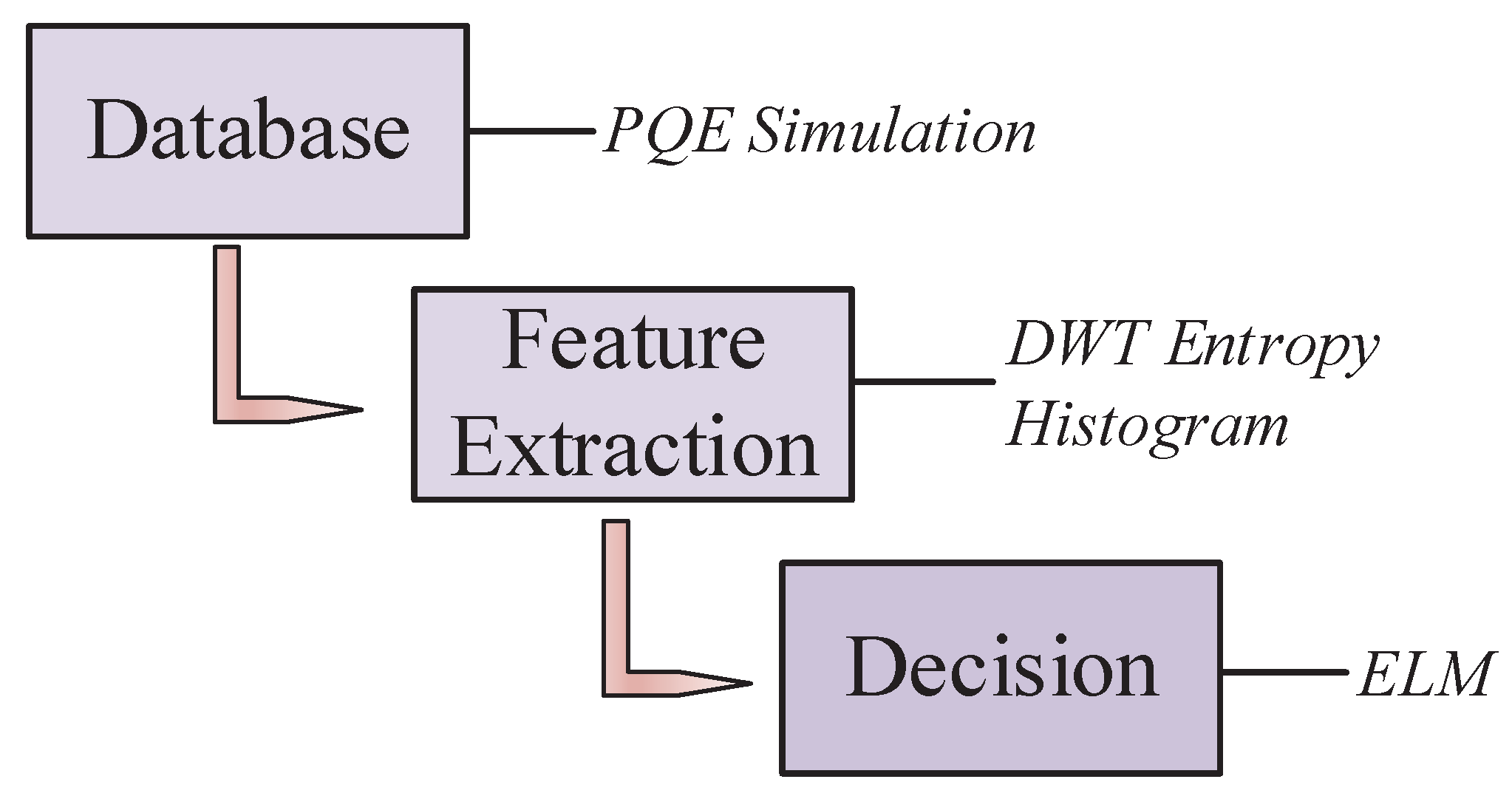In Figure 1, we present the general block sheme of the proposed intelligent event classification system. The three main steps—database construction, feature extraction and decision steps—are demonstrated with the included methods.

Following this chapter, the rest of this article is structured in this case: Section 2, Section 3 and Section 4 describe the methodology of FE and decision-making under the topics of DWT and the Entropy method, histogram, and ELM structure, respectively. Section 5 describes the PQE dataset and designated PQE generator; Section 6 emphasizes analyses and results of the proposed pattern recognition system. The last chapter is a brief conclusion for the study.

2. Feature Extraction: Wavelet–Entropy

WT operates a resilient time-frequency analysis and reveals the implicit partitions that signal includes. While FFT only performs frequency analysis, ST–FFT fills the gap and performs its analysis in the time-frequency domain. ST–FFT utilizes a fixed width window when tracking the signal. WT overcomes this issue by means of a scalable window width. Thus, analysis continues with extended window width to probe low-frequency divisions of signal and with reduced window width to probe high-frequency divisions. In power system signal processing, WT is a useful tool because it can clearly detect beginning and ending points of events [44]. WT governs a scalable wavelet model when healing the constant resolution affair and gives a flexible time–frequency analysis at different resolution levels [22,26,44,45,46]. The discrete form of WT is expressed as:

$$DWT(a,b)=2^{-a/2}\int y(t)\psi (2^{-a}t-b)dt,$$

(1)

where a is the scaling parameter of frequency, and b is a time offset. $y(t)$ represents the processed signal while $\psi (t)$ is the wavelet function. DWT method uses MRA, dividing the signal into lower frequency levels. Theoretically, levels of frequency sub–bands are unlimited whereas in practice sampling frequency restricts the levels of MRA [44]. In this study, 8-level decomposition is used in DWT MRA and the wavelet function is “Daubechies 4” ($db4$) based on former works in literature [5]. 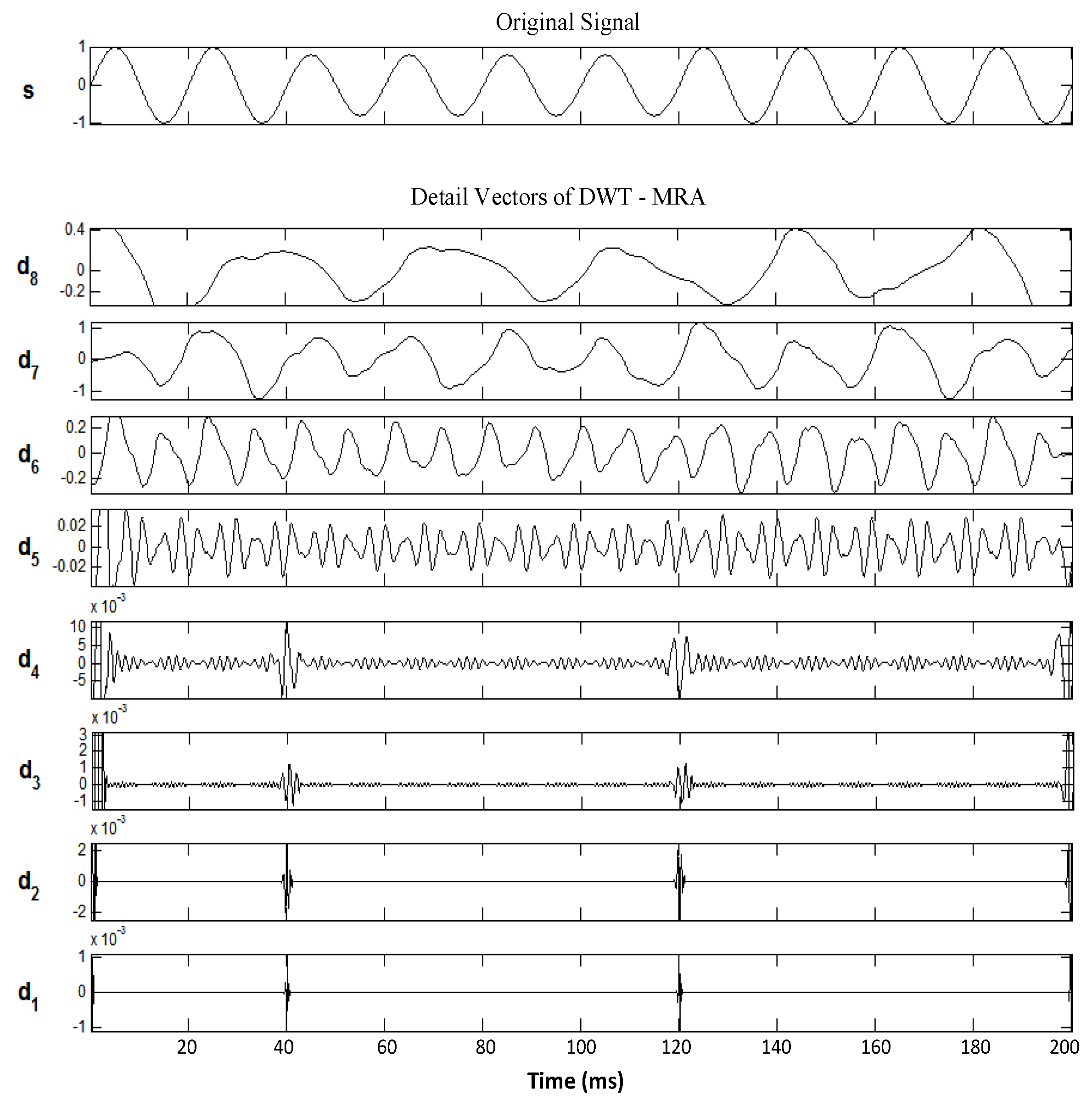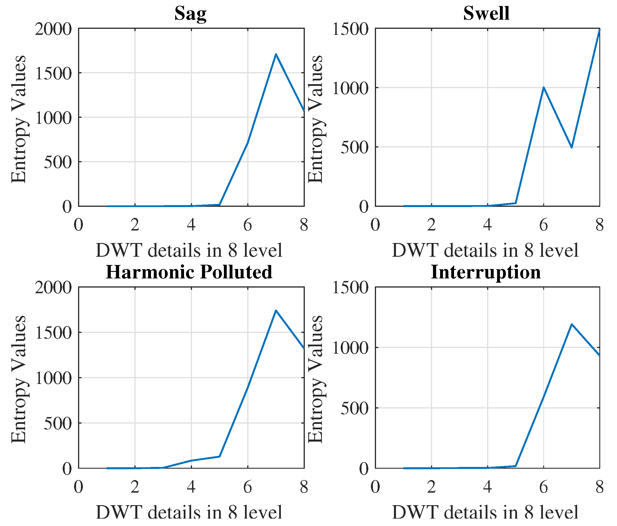Figure 2 shows DWT–MRA analysis in graphical representation for chosen sample events. As it can be seen in depth, details in $d_1$–$d_4$ range indicate start and end moments of PQE, clearly. In Figure 2, “s” is the raw signal.

Raw signals should be subject to a size reduction process before serving as classifier input. In this study, the entropy method is applied to detail vectors of DWT (for detail vectors, see Figure 2). In terms of statistical explanation, entropy states the “disorder” in a signal. The usage of signal processing field, Shannon is one of the first proponents of the entropy approach [47]. Entropy computation is an optimum way to measure the disorder in a non-stationary signal. Commonly used entropy calculations in signal processing are Shannon, Threshold, Norm, Sure method and Logarithmical Energy [46,48]. Shannon Entropy is preferred in this study, which is described as:

$$E(y)=\sum _i{y}_i^2·{log}_2(y_i^2),$$

(2)

where $y_i$ is the element of signal number i. Entropy computation generates eight features based on DWT coefficient vectors for each PQE.

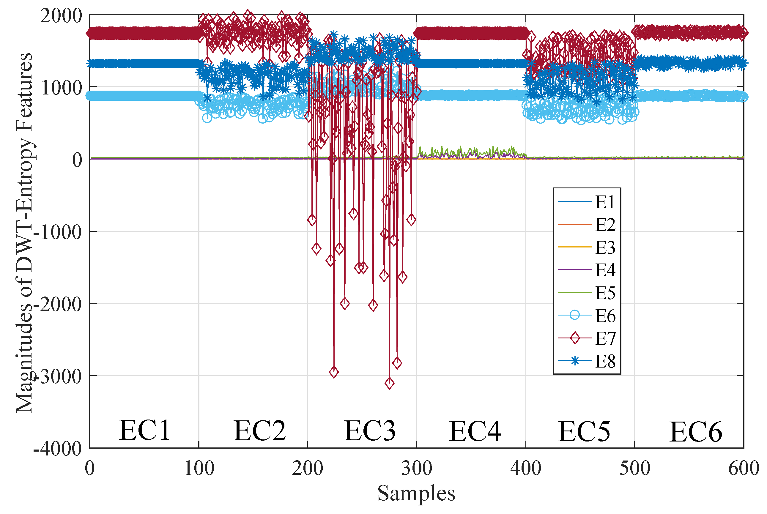
Figure 3 illustrates a graphical representation of DWT details’ entropy of four selected sample events in the dataset. It can be clearly seen that DWT–Entropy features characterize PQE data effectively. In this study, DWT is preferred for performance boosting of the histogram method.

3. Feature Extraction:Histogram

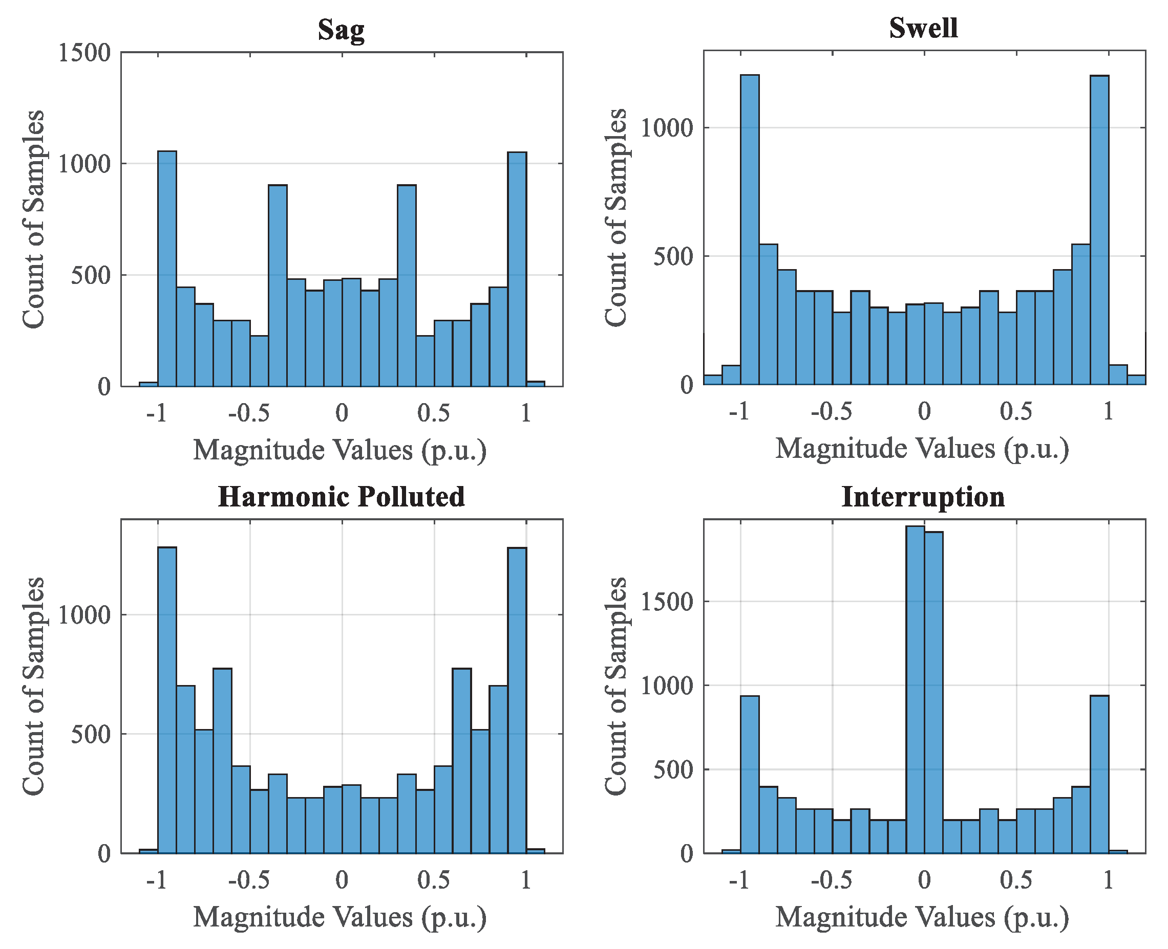
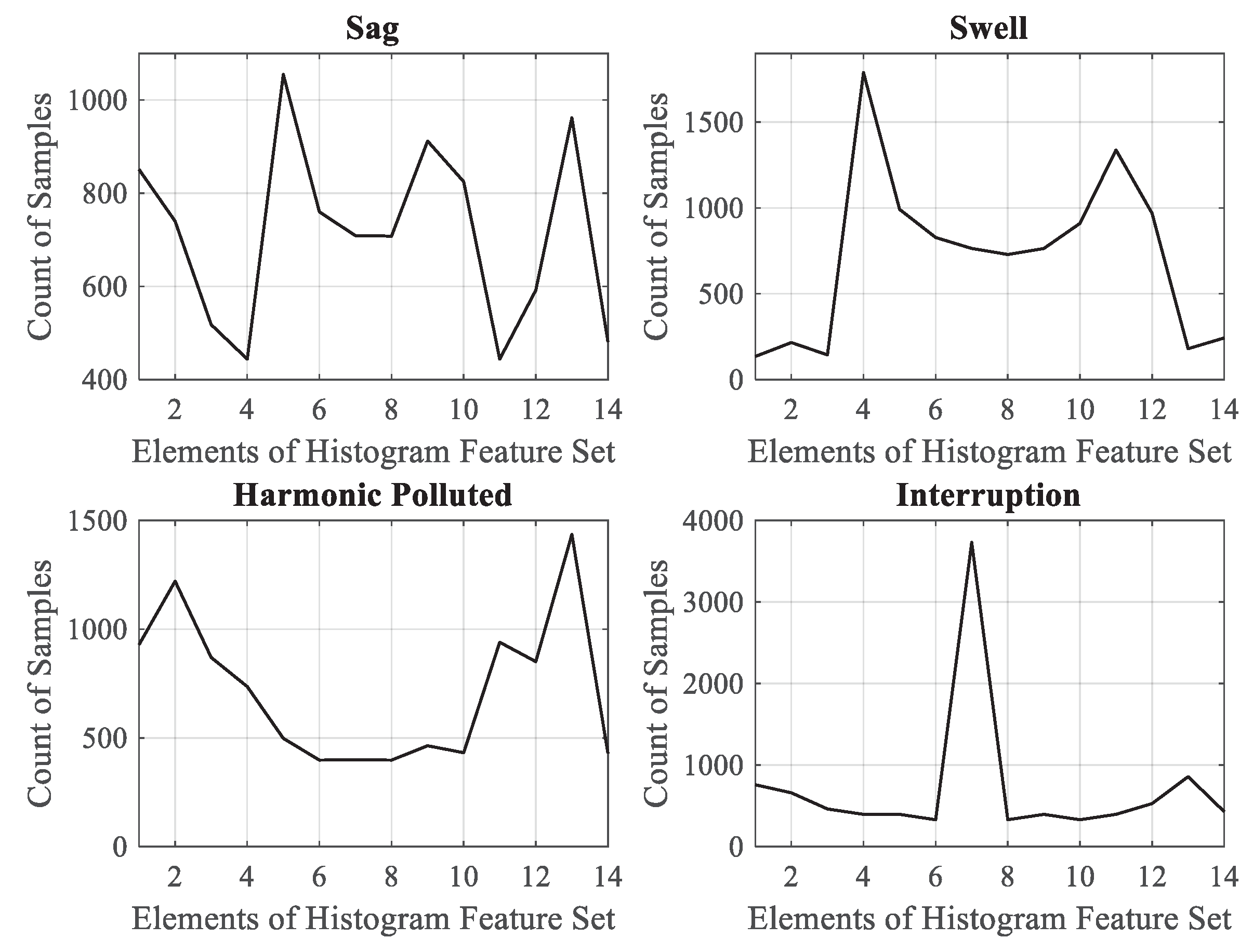
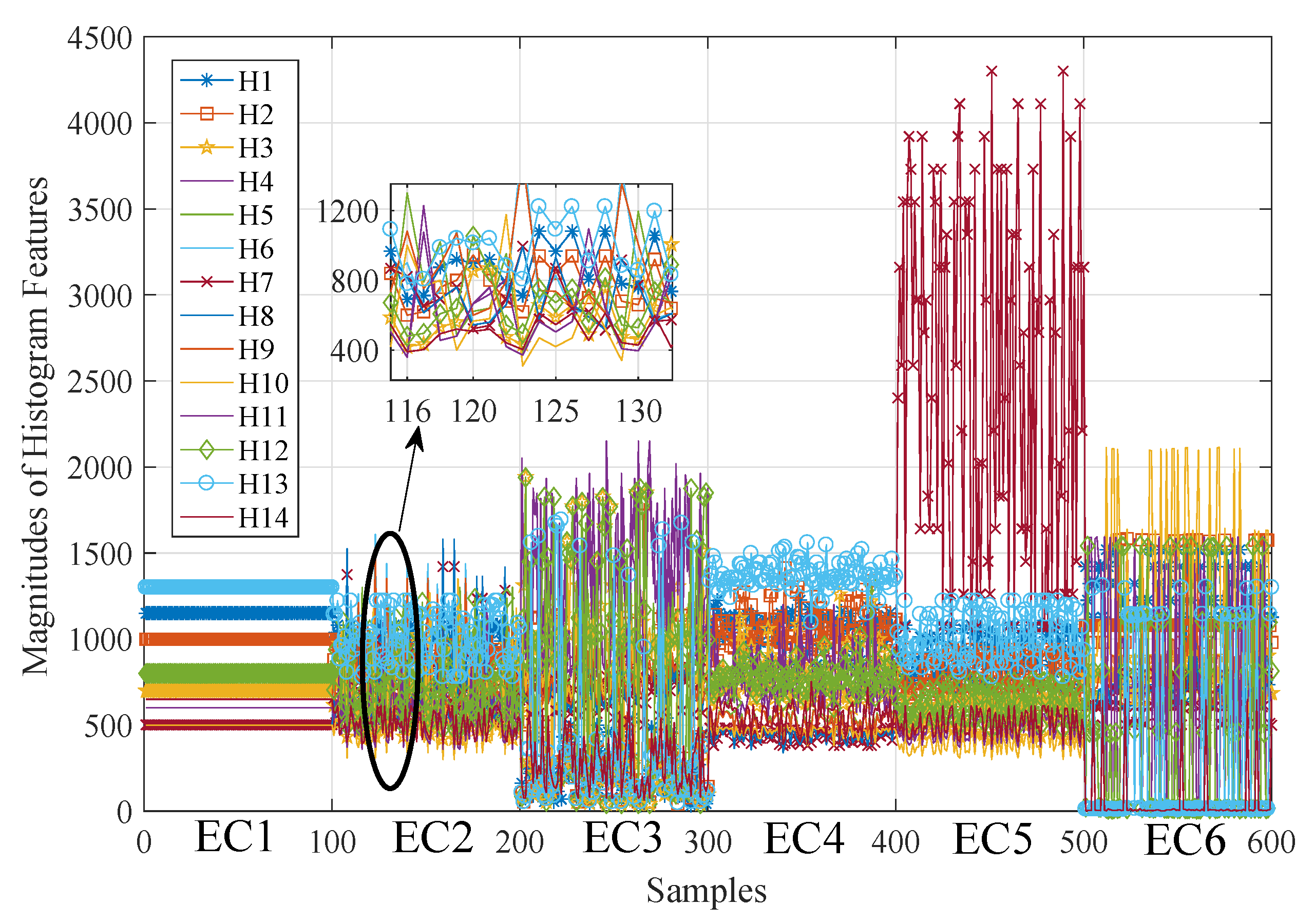
Using histogram, a graphical distribution is achieved that indicates the counts of samples in specific intervals throughout complete data array [30,49,50]. In our PQE dataset, histogram features characterize nearly whole events individually. Figure 4 illustrates the general histogram bars of sample events.

Figure 4 shows a unique distribution scene for each event, making feature extraction more distinctive.

In this study, counting points of each interval, so called “bins”, are specified by Sturges’ Rule, which is defined inclusively in [30]. With this designation according to Equation (3), the histogram feature set has consisted of 14 elements for each PQE , where C is the interval number and k is the samples of each signal here is 10.001. Figure 5 shows us histogram features of sample events:

$$C=1+3.322log(k).$$

(3)

As one can see in Figure 5, histogram features have the ability to emphasize nearly all PQE individually. Figure 5 includes the counts of signal magnitudes according to chosen 14 bins.

Algorithm 1 briefs the whole process of feature extracting. Algorithm 1 runs for every sample of the dataset, which is a number of 600.

Algorithm 1 Applied FE method using DWT–Entropy and histogram

Input: Loading PQE Dataset

Output: Total feature set to be classified

Feature Extraction :

1: for $i=1$ to 600 do 2:  Calculate the DWT details of PQE signals using (1), 3:  Calculate the Entropy values of DWT details with (2) 4:  Form the feature set $[E_1\dots E_8]$, 5:  Calculate the Histogram counts of PQE signals 6:  Form the feature set $[H_1\dots H_{14}]$ 7: end for 8: Compose the total feature vector $[E_1\dots E_8,H_1\dots H_{14}]$

4. Decision-Making: Extreme Learning Machine

ELM was firstly proposed by Huang et al. [34] and is a learning structure applied to SLFNs. In the ELM algorithm, weights and biases of the input layer are arbitrary while only the outputs are calculated [51]. The fact that the first layer is assigned arbitrarily has been stated, and the learning time for ELM is extremely short. Additionally, the ELM structure has accurate generalization ability compared to Feed Forward ANN (FF–ANN) based conventional learning algorithm [38,39]. 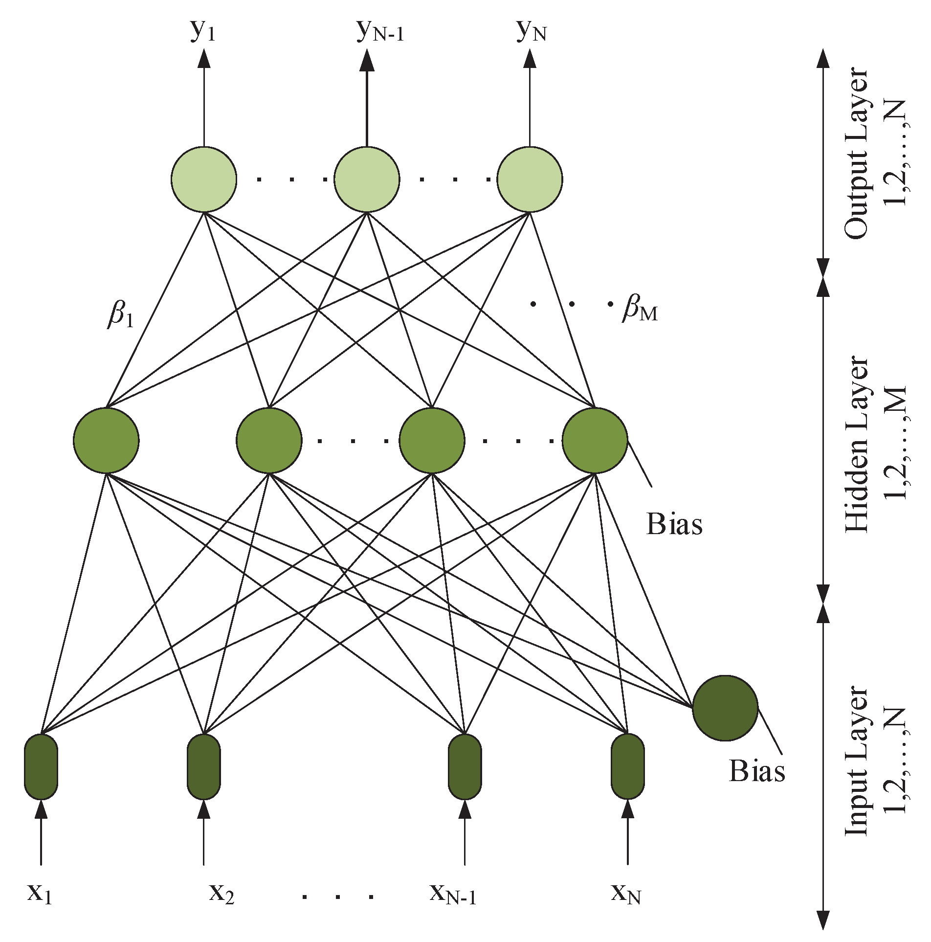Figure 6 briefs a basic SLFN frame. Inputs and outputs of the classifier are shown as $x_i$ and $y_i$.

The basic SLFN frame, which contains M total of hidden nodes and operates with $g(x)$ activation function, can be described in mathematical form as:

$$\sum _{i=1}^M{\beta }_{i}g(w_i·x_j+b_i)=o_j,j=1\dots N,$$

(4)

where w is the input weights of the layer, and $\beta$ is weights of the output layer. $b_i$ is bias values of the input layer. o defines the expected output of ELM. $(w_i·x_j)$ operand is the inner product of $w_i$ and $x_j$ so-called weighted inputs. Given the structure of SLFN can establish the “zero error” theoretically, i.e., o value is equal to y output vector. Thus, Equation (4) can be reformulated as:

$$\sum _{i=1}^M{\beta }_{i}g(w_i·x_j+b_i)=y_j,j=1\dots N.$$

(5)

Equation (5) exhibits that there are suitable output weights able to form measured outputs or real outputs of SLFN. If a facilitation is implemented as in (6), Equation (5) can be reformed as in (7):

$$\begin{array}{cc}\hfill g(w_i·x_j+b_i)& =H_{ij},\hfill \end{array}$$

(6)

$$\begin{array}{cc}\hfill Y& =H·\beta .\hfill \end{array}$$

(7)

Equation (7) refers to a linear equation whose solution takes us to output values of ELM. In usual learning frames, there is a need for iterative processes to obtain expected outputs, but ELM solves only a linear equation to execute the similar process at one time without any iteration. Equation (8) describes the solution for getting $\beta$ value from (7):

$$\beta =H^{◊}·Y,$$

(8)

where $H^{◊}$ is operated via the “Moore–Penrose inverse” so-called generalized inverse of H matrix [22,52].

Algorithm 2 briefs the ELM learning. In decision-making, we use the last feature vector with a length of 22 that includes eight features ($E_1,\dots ,E_8$) from DWT–Entropy and 14 features ($H_1,\dots ,H_{14}$) from the histogram method. Process loop runs for every sample of the dataset.

Algorithm 2 ELM Method

Input: Training set, $[t=1,2,\dots ,T]$,

Output: Output weights of ELM structure: Calculation of $\mathit{\beta }$ from $\mathbf{Y}=\mathbf{H}\mathit{\beta }$.

Initialisation :

1: Defining input weights and biases randomly. 2: for $t=1,2,\dots ,T.$ do 3:  Compute $\mathbf{H}$ matrix using (4) and (6), 4:  Compute the output weights from (8), 5: end for

Test :

6: Predict an unlabeled test input 7: Decide the type of PQE

5. Power Quality Event Data Description

The PQE simulation model presented in this paper has three steps: generating events using mathematical equations, normalization, and building last datasets to be processed. All three steps of the model have been designed in MATLAB [43]. Built simulation model generates five categories of voltage events such as sag, swell, interruption, harmonic polluted voltage, and flicker. In addition, a pure sinusoidal voltage is generated in order to depict normal operating conditions. PQE generator is operated at 10 kHz sampling frequency. Sampling frequency value can be thought of as measurement devices’ operating frequency. The built model composes the dataset using mathematical models of events [8,25]. The frequency of the grid model is considered as $50\mathrm{Hz}$; thus, a data array includes 200 samples in a period duration and measured time is set to 1-s. This operation time gives $1\times$ 10,001 length of raw data vector. The complete dataset includes six different classes for a total of 600 events, each with a length of 10,001 samples. At the end of the feature extraction process, the dataset is subject to a size reduction and as a result the feature vector has a length of 22 before processing in the classifier stage. In a 1-s period of an operation window, data rows have three sections as pre–event, event and post–event. Occurring durations are different from each other for every single event data. The built simulation model sets different durations of events in every data row. This makes every PQE unique in each class.

Table 1. Mathematical model based power quality event types and numbers.

PQE Type	Class	Number of Signals
Normal Sine	EC1	100
Sag	EC2	100
Swell	EC3	100
Harmonics	EC4	100
Interruption	EC5	100
Flicker	EC6	100
Total		600

briefs the dataset in terms of Event Class (EC) types.

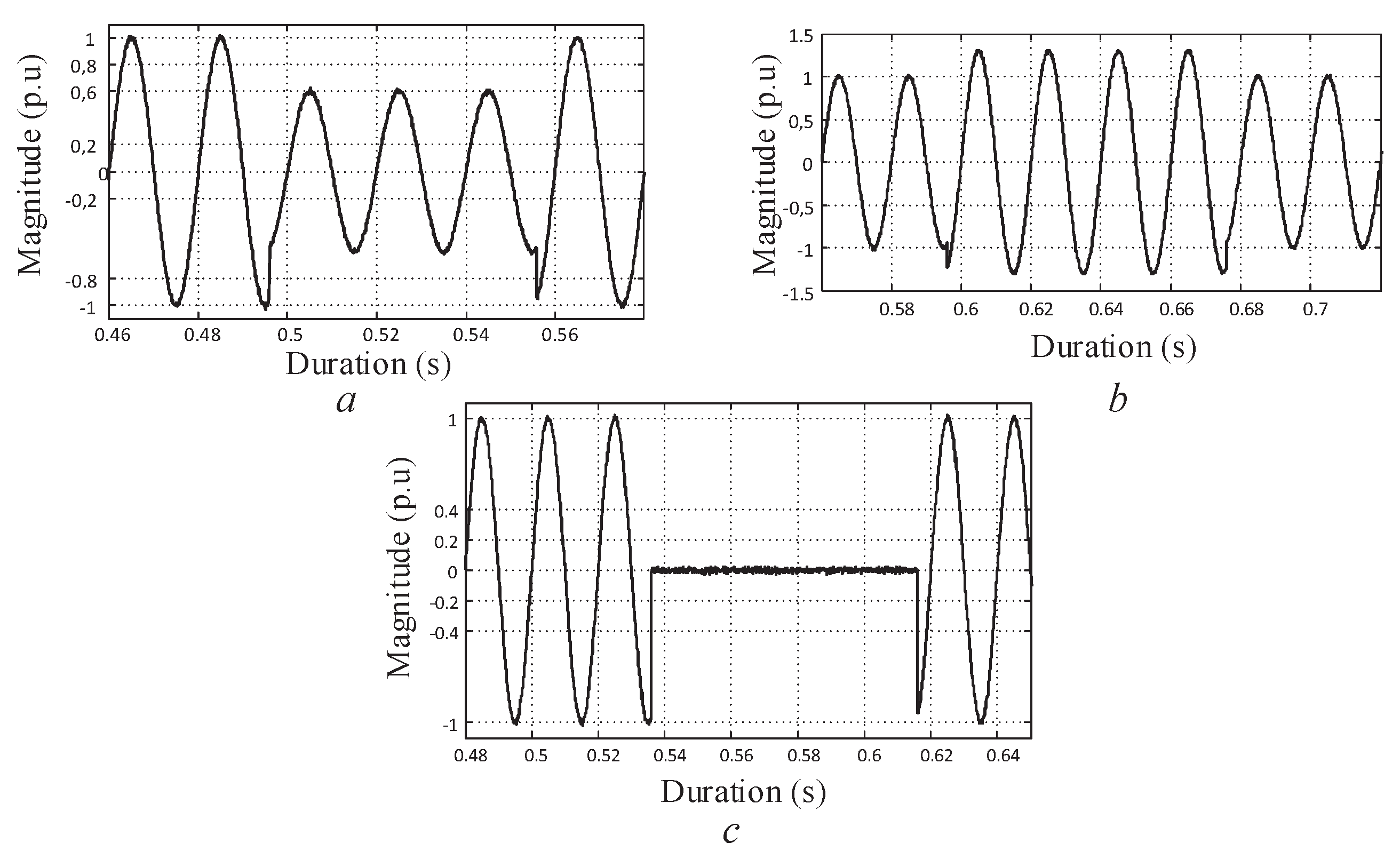
In order to resemble a real-field dataset, noise distortion is considered at values of Signal-to-Noise Ratio (SNR) 10 dB, 20 dB, and 30 dB. Noise addition makes dataset closer to real-site signals so that classifier performance is forced to various difficulty levels. Figure 7 illustrates three type of exemplary PQE signals in the dataset.

6. Results and Discussion

After feature extraction process using DWT–Entropy and histogram methods, a set of distinctive features is obtained to be classified in a decision-making phase. Whole feature set matrix includes $E_1,\dots ,E_8$ set as DWT–Entropy features, and $H_1,\dots ,H_{14}$ set as the histogram features. The feature matrix has a row number of 600, the same as samples of the dataset. In this study, a feature vector that consists of 22 elements is used for classification.

The feature set has a pre-processing period containing normalization and a cross-validation procedure. A 10-fold cross validation algorithm is used to get a better test performance and to force classifiers to more complicated test periods. Because of using cross-validation, accuracy values are given for 10-fold on average. FF–ANN and ELM have the same form as the SLFN structure. Because of this reality, we compare the proposed method just with the classic FF–ANN topology. In our experiments, number of hidden neurons are 225 and 20 for ELM and FF–ANN. Both classifiers use tangent sigmoid activation function in the hidden layer. Given parameters are acquired empirically as optimum values of several experiments. All the simulation is held by a work station hardware including a dual-processor with a clock of $2.1\mathrm{GHz}$ and $32\mathrm{GB}$ of RAM value. Results for SNR 10 dB, SNR 20 dB, and SNR30 dB are given using those classifier parameters above.

In

Table 2. The result table for signal-to-noise ratio 30 dB, 20 dB, and 10 dB conditions.

Classifier Type	Average Accuracy (%)	Time (s)
		Training	Test
Results for 30 dB Conditions
ELM	100	0.3266	0.0250
FF–ANN	99.0	0.9007	0.0111
Results for 20 dB Conditions
ELM	99.66	0.3141	0.0000
FF–ANN	98.00	0.8883	0.0262
Results for 10 dB Conditions
ELM	99.83	0.2906	0.0000
FF–ANN	99.17	0.9641	0.0138

, results for SNR 30 dB, 20 dB, and 10 dB noise conditions are presented collectively for both classifiers. It is said that ELM has a robust structure for different noise states. In Table 2, results for SNR 30 dB conditions show that ELM has a superior performance with $100\%$ accuracy and classifies all the classes correctly. In addition, ELM is good at a time cost in both training and test phases. FF–ANN has an adequate performance, but it is nearly three times slower in the training period. This time costs when processing the big data concept. In Table 2, we can see the accuracy performance of SNR 20 dB as $99.66\%$. In Ref. [8], the performance value that belongs to the same condition is $96.22\%$. Using an easy to implement method with less features and less computational time, our proposed system outperforms the DGT with type-2 fuzzy based SVM. Because our classifier demonstrates its robustness in Table 2 with different noise levels, we set the SNR 30 dB value as the benchmark level. Other result tables present the results with the benchmark noise level as SNR 30 dB.

When making a comparison between two similar classifiers, it is always considered whether the test is running under equal circumstances. The results carried out using the optimal classifier parameters are above. In this part of the experiments, two more different operation conditions are provided for classifiers: (1) when ELM has a number of 20 hidden layer neurons just the same as FF–ANN; and (2) when FF–ANN has a number of 225 hidden neurons just the same as ELM. This allows both classifiers for evaluating with the same situations.

Table 3. The result table for SNR 30 dB and both ELM & FF–ANN are under equal terms of neuron numbers.

	20 Neurons			225 Neurons
Classifier	Average Accuracy (%)	Training Time (s)	Testing Time (s)	Average Accuracy (%)	Training Time (s)	Testing Time (s)
ELM	97.50	0.0578	0.0000	100	0.3266	0.0250
FF–ANN	99.00	0.9007	0.0111	96.00	129.353	0.0325

presents the results of those two conditions.

The most important argument of this evaluation approach is about time cost of FF–ANN. In Table 3, when FF–ANN has 225 neurons, training time is nearly four hundred times more. In comparison with FF–ANN, when ELM has 20 neurons, it generates nearly accuracy of $98\%$ with a fast training time. Dealing with a large-scale dataset, training time is a crucial value of interest.

The results above are obtained via using of the full feature set. Now, the ongoing analysis has a feature searching starting with DWT–Entropy features. Figure 8 shows $E_1,\dots ,E_8$ feature sub-set for all the samples of the dataset.

One can see from Figure 8 that $E_1$ to $E_5$ features are less distinctive comparing to $E_6$ to $E_8$ features. Magnitudes of $E_1$–$E_5$ are low values and show a little change only for $EC4$ class, but $E_6$–$E_8$ features differ from each other for all the classes of the dataset.

Table 4. ELM results for DWT–Entropy features (SNR 30 dB).

Feature Set	Average Accuracy (%)	Time (s)
		Training	Test
$E_6$–$E_8$	72.70	0.3609	0.0156
$E_1$–$E_5$	63.80	0.3094	0.0000
$E_1$–$E_8$	96.20	0.3563	0.0000

shows the ELM results of classification using only DWT–Entropy for SNR 30 dB with different combinations.

The meaning of Table 4 differs from graphical projection. Figure 8 tells us that $E_1$–$E_5$ features are less distinctive but classification results refute that estimation. Using just $E_6$–$E_8$ features gives $72.7\%$ of average accuracy. When $E_1$–$E_5$ features are added and using the whole DWT–Entropy sub-set, average accuracy rises to $96.2\%$ value and the result for using only $E_1$–$E_5$ sub-set has an average accuracy of $63.8\%$.

General distribution of the histogram features is given in Figure 9. It can be clearly seen that all histogram features ($H_1$–$H_{14}$) are distinctive for nearly all classes. The features of $EC2$ are less distinctive among all feature sub-sets, but if we zoom in its distribution, it is seen that they differ from each other.

Now, the next results are obtained using just the histogram features, $H_1$–$H_{14}$.

Table 5. ELM result table for histogram features (SNR 30 dB).

Feature Set	Average Accuracy (%)	Time (s)
		Training	Test
$H_1$–$H_{14}$	98.70	0.3734	0.0266

lists the ELM classification according to $H_1$–$H_{14}$ feature sub-set with SNR 30 dB. The histogram feature sub-set with an average accuracy of $98.7\%$ is adequate for the proposed PQE classification system.

A general comparison is given in

Table 6. Feature extraction method comparison.

Method	Feature Set Length	Processing Time (s)	Average Accuracy of ELM (%)
DWT–Entropy	8	7.66	96.2
Histogram	14	0.51	98.7
Total feature set	22	8.2	100

according to processing time and average accuracy values; specs of total feature sets are also listed. As it can be seen in Table 6, extracting features from the histogram method is 15 times faster than DWT–Entropy. Average accuracy values are close to each other so the important point is time cost, most particularly dealing with big data. For the whole feature set, the proposed system for PQE classification reaches the perfect classification. However, the proposed intelligent recognition system can be used just preferring the histogram method based feature set, which is the novelty of this paper. Its accuracy reaches an adequate performance value and the DWT method supports this for more.

7. Conclusions

In this paper, a machine learning based ELM classifier coupled with DWT–Entropy and histogram methods for classification of PQE signals is proposed. With its MRA nature, the DWT method is used to establish a time-frequency analysis suitable for event signals. Feature extraction from DWT is based on entropy calculation. This study proposes the histogram, which is a novel feature extracting method used in power system signal processing with a machine learning based classifier. Histogram features characterize PQE data in an accurate manner. Feature extraction methods provide a size reduction in the raw dataset before classification process. In addition, the proposed feature extraction method of histogram comes to the fore with being fast in time, and its easy implementation for embedded systems. Designing a power quality event monitoring device using just histogram features is one of the future aims of this study. The conventional DWT method is used for performance improvement of the histogram. Given results prove the increase in performance.

The results from the proposed pattern recognition system prove that it carries an efficient classification process with six categories of PQE. In addition, it can be said that the proposed system has a robust structure for different noisy conditions. Future works will include building an embedded system for the histogram method. Thus, it would be able to run the algorithm on a field device.