Validating a Wave-to-Wire Model for a Wave Energy Converter—Part I: The Hydraulic Transmission System

Abstract

Considering the full dynamics of the different conversion stages from ocean waves to the electricity grid is essential to evaluate the realistic power flow in the drive train and design accurate model-based control formulations. The power take-off system for wave energy converters (WECs) is one of the essential parts of wave-to-wire (W2W) models, for which hydraulic transmissions are a robust solution and offer the flexibility to design specific drive-trains for specific energy absorption requirements of different WECs. The potential hydraulic drive train topologies can be classified into two main configuration groups (constant-pressure and variable-pressure configurations), each of which uses specific components and has a particular impact on the preceding and following stages of the drive train. The present paper describes the models for both configurations, including the main nonlinear dynamics, losses and constraints. Results from the mathematical model simulations are compared against experimental results obtained from two independent test rigs, which represent the two main configurations, and high-fidelity software. Special attention is paid to the impact of friction in the hydraulic cylinder and flow and torque losses in the hydraulic motor. Results demonstrate the effectiveness of the models in reproducing experimental results, capturing friction effects and showing similar losses.

1. Introduction

Wave energy is one of the potential suppliers of clean energy in a future de-carbonised power sector along with other more developed sources, such as solar-, wind- or hydro-power. However, if wave energy is to compete with these more developed energy sources on an equal footing, it is necessary that wave energy maximises the final energy output to minimise the cost of energy.

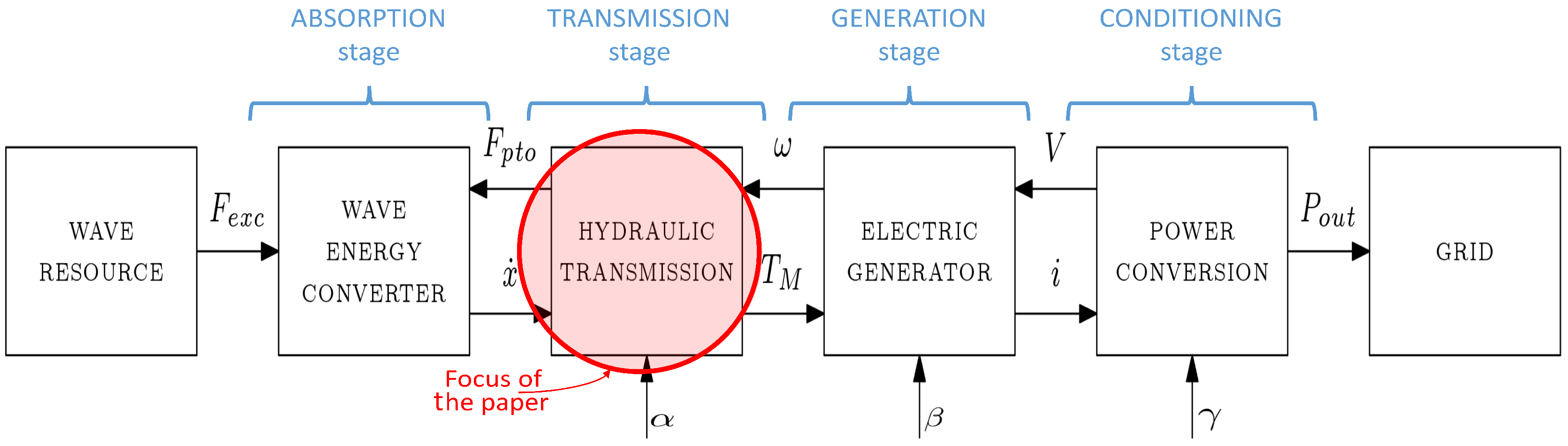
To analyse realistic final energy generation and design accurate model-based control strategies for wave energy converters (WECs), it is crucial to examine the whole chain from waves to the electricity grid. Hence, accurate mathematical models that incorporate all the necessary components of the different conversion stages from waves to the grid, known as wave-to-wire models (W2W), are necessary. Figure 1 shows the different stages of that chain that need to be incorporated in the W2W models, including the control inputs for each stage ($\alpha$, $\beta$ and $\gamma$). The most important aspects of all conversion stages in W2W models are reviewed in [1] for different power take-off (PTO) configurations: pneumatic [2], hydraulic [3] or mechanical transmission systems [4] coupled to a rotational generator, or even direct drive systems with linear generators [5].

Although diverse PTO systems have been suggested by different wave energy researchers and developers, hydraulic PTO transmission systems appear to be the choice of the vast majority of developers, including Pelamis [6], Searev [7], Wavestar [8], Oyster [9], CETO [10] or Waveroller [11]. The present paper focuses on wave-to-wire models with hydraulic transmission systems.

The W2W model validated in the present paper is designed as a combination of inter-connected sub-models, where each sub-model can take a different time-step by implementing multirate time-integration schemes [12,13]. That way, components with faster dynamics can take shorter time-steps without adding unnecessary computations to the slower components.

The large number of components included in W2W models makes the validation of W2W models, as a whole, quite challenging, mainly due to the complexity and cost of building a physical model with all the components. Therefore, the authors decided to accomplish the validation by separately validating each conversion stage of the model, which is consistent with the way the W2W model is designed.

The hydrodynamic model of the absorption stage is validated against high-fidelity software in [14], where a heaving point absorber is examined when moving with and without control. The validation of the mathematical models for the transmission, generation and conditioning stages is divided into two parts and is presented as a series of two papers. The first paper (Part I), the present paper, shows the validation of the transmission stage, as highlighted in Figure 1, and the second paper (Part II) presents the validation for the generation and conditioning stages [15].

1.1. Hydraulic Transmission Systems in Wave Energy

Several topologies of hydraulic system have been suggested for wave energy converters in the literature. The most simple hydraulic transmission systems include a hydraulic cylinder, high- and low-pressure accumulators, a rectification bridge and a fixed-displacement hydraulic motor, as suggested in several studies, such as the W2W models presented in [7,16,17,18], and also in [19], where a W2W model for arrays is proposed.

In order to improve the performance of that ‘standard’ system, alternative configurations have been suggested in the literature. Four configurations with higher flexibility are presented in [20], where the main difference among the four configurations is the arrangement of the accumulators. Another topology with direct connection between the hydraulic cylinder and a variable-displacement motor is suggested in [21], while a configuration using a multi-chamber hydraulic cylinder connected to multiple accumulators, with different pressure settings (which, in turn, are connected to a fixed-displacement motor), is presented in [22].

All these topologies can be organised in two main groups [23]: constant- and variable-pressure configurations.

1.1.1. Constant-Pressure Configuration

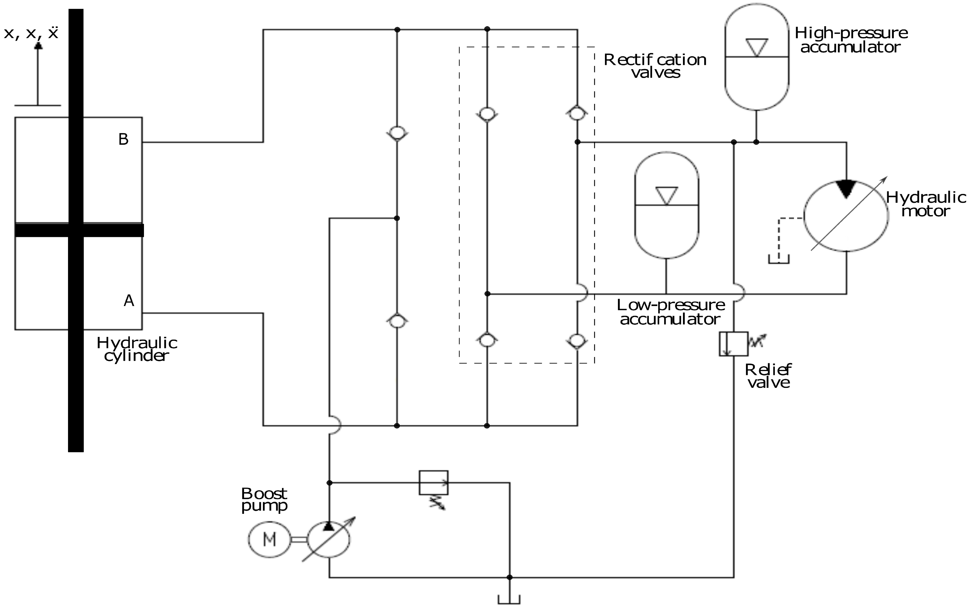
The typical constant-pressure configuration is described in [24]; and generally includes a hydraulic cylinder, a set of check-valves for the rectification of flow, low- and high-pressure (LP and HP, respectively) accumulators, a hydraulic motor, a relief valve, and a boost pump powered by an electric motor, as illustrated in Figure 2. The reciprocating motion of the WEC and, as a consequence, of the cylinder piston, is rectified by means of the rectification valves, so that the hydraulic motor operates in a single quadrant, meaning that the direction of the motor rotation and torque is always the same. The HP and LP accumulators dictate the pressure difference in the cylinder and help to provide a smooth and slowly varying torque in the hydraulic motor. Relief valves only open when the pressure in the system exceeds the maximum pressure allowed by the different components of the system and the boost pump ensures that the pressure in the system never falls below a pre-defined minimum pressure level, avoiding undesirable effects such as cavitation.

Hydraulic transmission systems based on the constant-pressure configuration have, in general, quite limited controllability. The only controllable variable in such constant-pressure hydraulic systems ($\alpha$ in Figure 1) is the displacement of the hydraulic motor. However, the use of large HP accumulators connected to the hydraulic motor constrains the whole system to perform in constant-pressure, meaning that variations in the motor displacement take a long time to affect the pressure in the hydraulic cylinder, and, eventually, the behaviour of the WEC. As a consequence, the overall power absorption in the wave energy converter can be rather poor, with limited possibilities for improvement. Only the use of extra (smaller) accumulators beside the hydraulic cylinder, as described in [16], can improve the power absorption, implementing control strategies such as latching or declutching, as shown in [25].

In spite of the limited controllability, the efficiency of constant-pressure hydraulic PTO systems can be reasonably high, since components can be controlled to perform close to the optimal operating point most of the time.

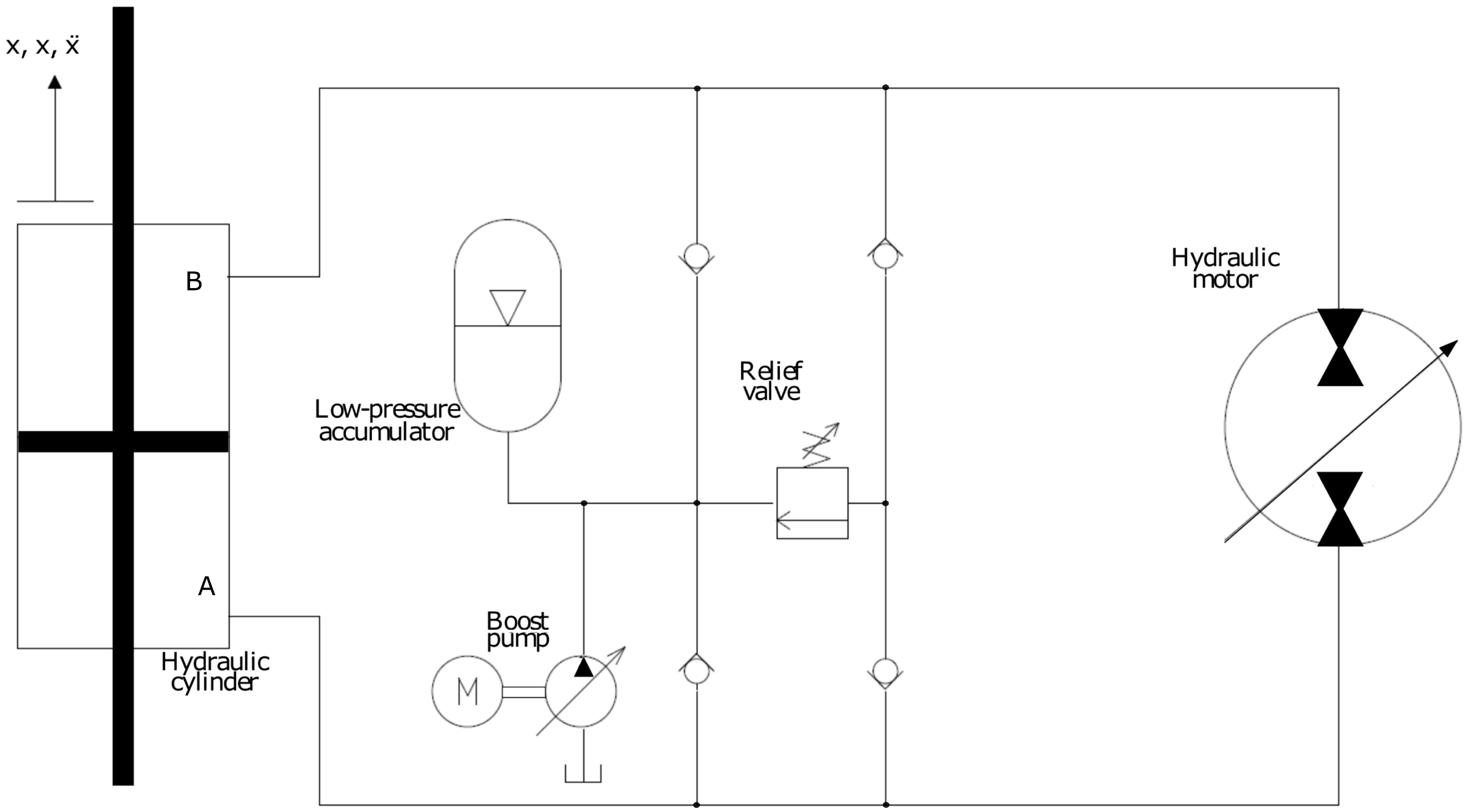
1.1.2. Variable-Pressure Configuration

The typical alternative to the constant-pressure configuration is shown in Figure 3, where the hydraulic cylinder is directly connected to a variable-displacement hydraulic motor. Only the LP accumulator is included in this configuration, which, along with the boost pump, avoid pressure drops in the low-pressure line, which can lead to undesirable situations, such as cavitation. A boost pump is also necessary to replenish the fluid leaks in the motor. Relief valves protect the system from over pressure, likewise in the constant-pressure configuration. In the variable-pressure PTO configuration, the reciprocating motion of the WEC and the cylinder piston is not rectified, obliging the hydraulic motor to operate, at least, in two-quadrants. The most common two-quadrant operation of the PTO system in WECs is that of a reversing torque and an irreversible rotation direction.

The absence of an HP accumulator provides a more flexible hydraulic system, increasing the control bandwidth. In the most basic form of a variable-pressure topology, cylinder ports are directly connected to the motor ports without any rectification system, i.e., the check-valves used in the constant-pressure configuration. Hence, variations in the hydraulic motor displacement rapidly affect the behaviour of the WEC, which allows for an effective control of the PTO force applied on the WEC to maximise power absorption from ocean waves. However, the motor may require four-quadrant operation capabilities to compensate for bi-directional flow.

The system shown in Figure 3 is close to the simplest version of a variable-pressure configuration. Similar configurations have been suggested in [20,21], including an energy overflow system connected to the relief valves. That way, when the cylinder produces more flow than the hydraulic motor can handle, the extra flow can be used to generate electricity, instead of leaking it to the LP accumulator, wasting energy contained in the HP fluid.

Further improvements of hydraulic transmission systems for wave energy converters combine the benefits of the constant-pressure and variable-pressure configurations, such as incorporating multiple HP accumulators with different pressure levels to achieve discrete force levels adapting the displacement of a variable-displacement motor [20]. Similarly, Ref. [22] incorporates multiple accumulators, but uses a fixed-displacement motor, where discrete force levels are achieved by means of a multi-chamber cylinder.

The mathematical models for the two configurations are significantly different, thus requiring separate validation. Therefore, experimental data, generated by using two different test-rigs, are used in the validation. The performance of the hydraulic cylinder for both hydraulic system configurations is validated against experimental results, while the well-known simulation software AMESim (v14.1, LMS/Siemens PLM Software, Leuven, Belgium) [26] is used to validate the performance of the hydraulic motor, due to the lack of experimental results for the hydraulic motor.

The paper is organised as follows: the mathematical models are described in Section 2, the experimental test-rigs are described in Section 3, results of the validation are given in Section 4; and conclusions of the validation are drawn in Section 5.

2. Mathematical Models for System Components

Mathematical equations to model the different components included in hydraulic transmission systems, i.e., hydraulic cylinders, valves, accumulators and hydraulic motors, are common to any hydraulic system configuration or topology. Therefore, the equations for the different components are given in the following subsections, regardless if such components are used in the constant- or variable-pressure configuration. The model structures used for each component are generic, in the sense that components of different characteristics, e.g., a hydraulic gear motor or a hydraulic radial piston motor, can be modelled using the same model structure. However, due to the very specific characteristics of each component, the parameters of the models may need to be fitted for each specific component.

2.1. Hydraulic Cylinder

Hydraulic cylinders, symmetric or asymmetric, consist, in general, of a piston that divides a cylinder into two chambers. Hence, pressure difference between the two chambers, imposed by the pressure in HP and LP accumulators in constant-pressure configurations and the torque-control implemented in the hydraulic motor in variable-pressure configurations, determines the cylinder force ($F_{PTO}$) applied on the WEC. The pressure dynamics can be described by means of the continuity equation given by the following expression:

$${\dot{p}}_A=\frac{{\beta }_{eff}\left(p_A\right)}{V_A+A_p{x}_p}(Q_A-{\dot{x}}_p{A}_p),$$

(1)

$${\dot{p}}_B=\frac{{\beta }_{eff}\left(p_B\right)}{V_B-A_p{x}_p}({\dot{x}}_p{A}_p-Q_B),$$

(2)

where $p_A$ is the pressure in the cylinder chamber A, $Q_A$ the flow entering or exiting the cylinder chamber A when leakages are neglected, ${\beta }_{eff}\left(p_A\right)$ the effective bulk modulus of the fluid and $V_A$ the minimum volume (calculated when the piston reaches its minimum or maximum position) in chamber A. Subscripts A and B refer to chambers A and B in Figure 2 and Figure 3. In addition, $A_p$ is the piston area, and $x_p$ and ${\dot{x}}_p$ are the piston position and velocity, respectively.

Equations (1) and (2) ignore both friction and inertia effects, which can represent between 5% and 10% of energy losses in the cylinder. As a result, the piston force only considering the pressure difference can result in an under-estimate of the force applied to the WEC. A more accurate representation of this force is given by

$$F_{PTO}=A_p(p_B-p_A)+F_{fric}+F_{in},$$

(3)

where $F_{fric}$ is the friction force and $F_{in}$ the inertia force. $F_{in}$ includes the inertial force of the piston, the rod and the oil, and the gravity force due to the mass of the piston and the rod:

$$F_{in}={\ddot{x}}_p(M_p+M_r+M_{oil})+(M_p+M_r)g,$$

(4)

where $M_p$, $M_r$ and $M_{oil}$ are the mass of the piston, rod and oil in the chambers, and g is the acceleration due to the gravity.

Friction Model

Friction is considered to be one of the main nonlinearities of the cylinder. Several different models have been suggested in the literature to describe friction losses in hydraulic cylinders, including static and dynamic models [27].

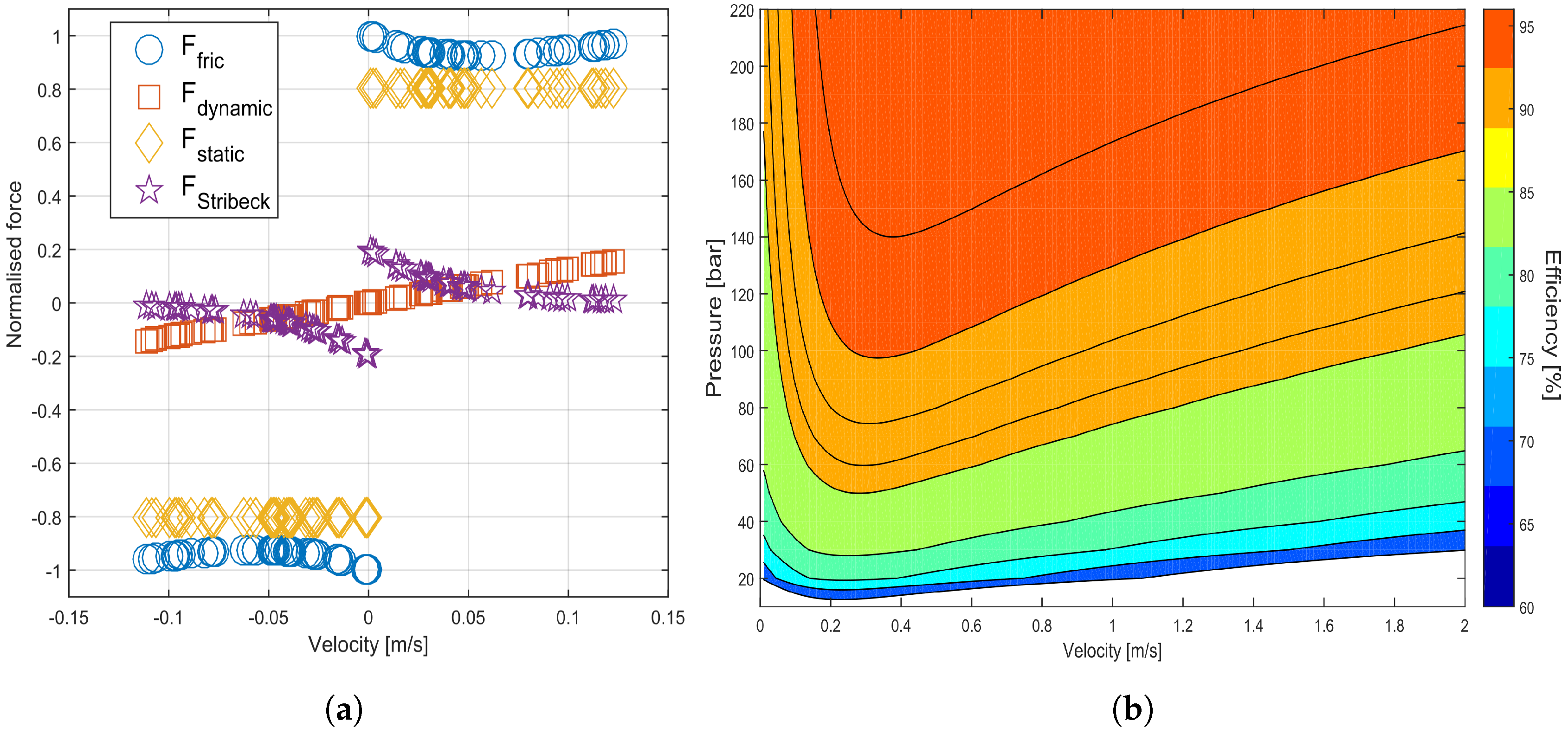
The vast majority of the models divide the friction model into different effects, i.e., viscous friction, Coulomb friction and static friction. A model, known as Stribeck model, combines the three effects as follows [28]:

$$F_{fric}=\sigma {\dot{x}}_p+sign\left({\dot{x}}_p\right)\left[F_c+F_{st}exp\left(-\frac{|{\dot{x}}_p|}{c_{st}}\right)\right],$$

(5)

where $\sigma$ is the viscous coefficient, $F_c$ the Coulomb friction force, $F_{st}$ the static friction force and $c_{st}$ the characteristic velocity of the Stribeck curve. Figure 4a illustrates the contribution of each friction effect normalized against the maximum friction force.

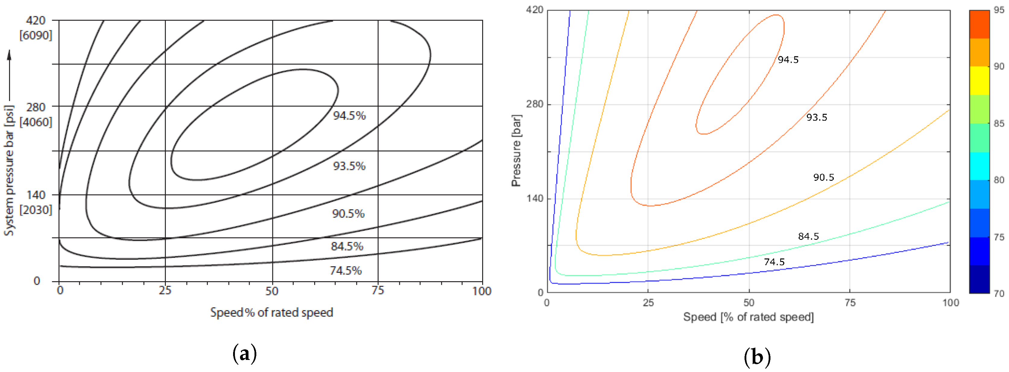
Once the model structure is selected, the parameters ($\sigma$, $F_c$, $F_{st}$ and $c_{st}$) of the model need to be defined. The most appropriate way to proceed would be fitting such parameters using experimental data from the cylinder to be implemented in real life. However, experimental results are not always available, so parameters need to be identified using other relevant information, such as manufacturers’ data. Therefore, the parameters for the present model are identified using an efficiency map as a function of velocity and pressure difference presented in [20], using the nonlinear least squares fitting technique. Figure 4b shows the efficiency map of the hydraulic cylinder, reproduced with the model parameters fitted from [20].

The friction model presented in this section assumes friction losses are symmetric, as shown in Figure 4a. However, this is not always true, especially in asymmetric cylinders. In some cases, a lag exists between the pushing (positive velocity) and retracting (negative velocity) forces. To include such asymmetry, the model structure presented in Equation (5) is still useful, but needs to be duplicated to distinguish the performance during the pushing and retracting operations, separately identifying the parameters for each operation [28].

2.2. Valves

Valves are essential components for the successful performance of hydraulic PTO systems, required to rectify or control the flow at different points of the circuit. Active and passive vales can be included in the hydraulic system, depending on the purpose of the valve, and both can be described using the orifice equation [28]:

$$Q_v=C_d{A}_v(\Delta p_v)sign(\Delta p_v)\sqrt{\frac{2}{{\rho }_{oil}}|\Delta p_v|},$$

(6)

where $Q_v$ is the flow through the valve, $C_d$ the discharge coefficient, $A_v(\Delta p_v)$ the valve opening area as a function of the pressure difference between the outlet and inlet ports of the valve, ${\rho }_{oil}$ the density of the hydraulic oil and $\Delta p_v$ the pressure difference between the inlet and the outlet of the valve.

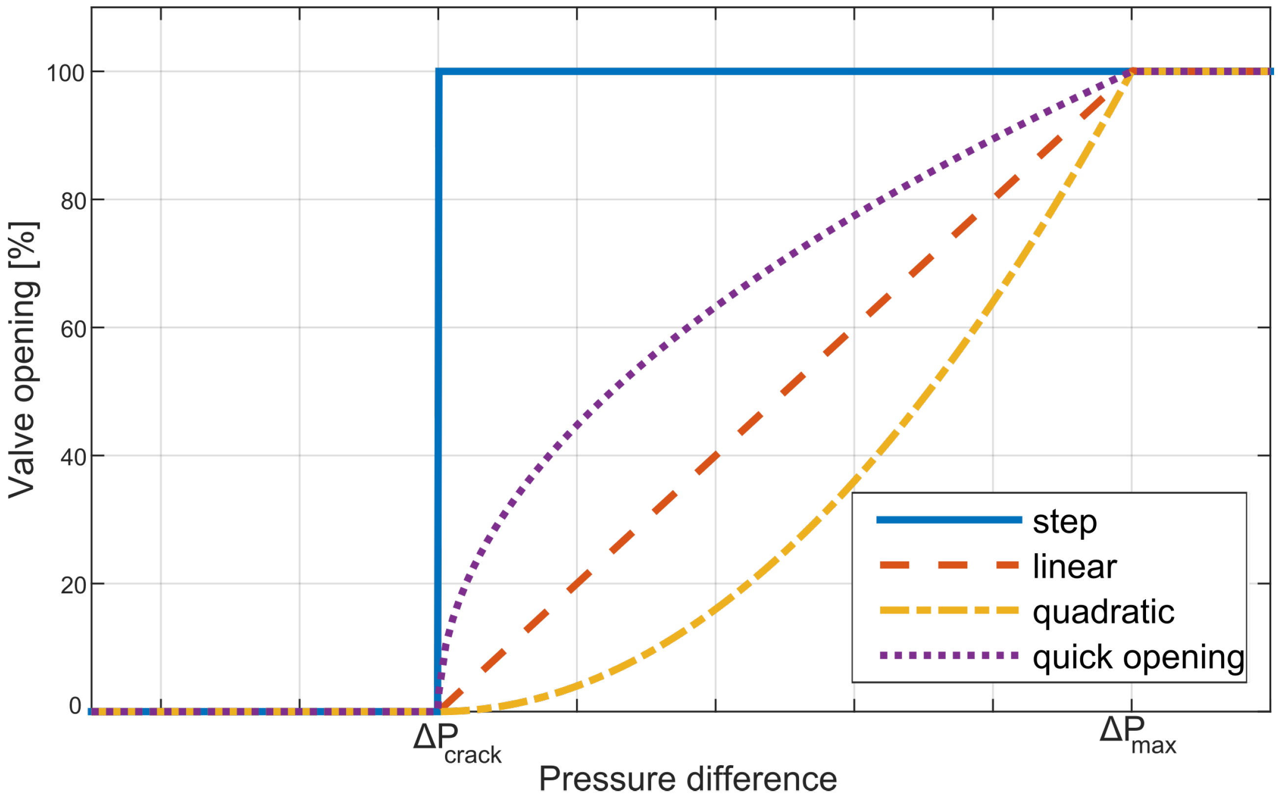
Only passive valves, check valves in the rectification bridge and relief valves are used in the present study, which open and close as a function of the pressure difference across the valve, as expressed in Equation (6). The valve remains closed while the pressure difference across the valve is lower than the cracking pressure ($\Delta p_{crack}$). Once the the cracking pressure is reached, the valve starts to open and continues opening until the valve is fully open. The pressure at which the valve is fully open is known as the maximum pressure ($\Delta p_{max}$). Hence, maximum area of the valve, and cracking and maximum pressure are, in general, provided in the manufacturers’ catalogues. However, the valve opening, from fully closed to fully open, can follow different profiles. Some of the most commonly observed profiles [29] are illustrated in Figure 5. In the model validated in this paper, the step function is implemented to reproduce the same valve opening profile as in the original study, where the experimental data is taken from [30].

2.3. Accumulators

The performance of hydraulic accumulators, typically compressed gas accumulators, can be described by means of an isentropic and adiabatic process, where volume of the hydraulic fluid contained in the accumulator changes in time as follows:

$$V_{acc}\left(t\right)={\int }_0^t{Q}_{acc}^{in}\left(t\right)dt,$$

(7)

where $Q_{acc}^{in}\left(t\right)$ is the input flow to the accumulator. Hence, following isentropic compression, the pressure in the accumulator is given by

$$p_{acc}=P_{pre}{\left(\frac{V_{tot}}{V_{gas}}\right)}^{\gamma },$$

(8)

where $p_{pre}$, $V_{tot}$ and $V_{gas}$ are the pre-charge pressure, the total volume and volume of compressed gas in the accumulator, respectively, and $\gamma$ is the adiabatic index for an ideal gas.

2.4. Hydraulic Motor

As pressure increases in the cylinder chamber, oil flows from the cylinder to the motor (through the check-valves and HP accumulator, in the case of the constant-pressure configuration), where pressure and flow discharged from the cylinder are converted into mechanical torque and rotation of the shaft. Once the motor extracts the energy from the high-pressure fluid, low-pressure oil flows back to the cylinder. The torque generated in the hydraulic motor ($T_M$) and the output flow ($Q_M$) can be expressed, respectively, as,

$$T_M=\alpha D_{\omega }\Delta p_M-T_{losses},$$

(9)

$$Q_M=\alpha D_{\omega }{\omega }_M-Q_{losses},$$

(10)

where $\alpha$ is the motor displacement fraction, $D_{\omega }$ the displacement of the hydraulic motor, ${\omega }_M$ the rotational speed of the shaft, and $\Delta p_M$ the pressure difference between the inlet and outlet ports of the hydraulic motor.

Motor Losses

Modelling mechanical ($T_{losses}$) and volumetric losses ($Q_{losses}$) in the motor, due to friction and leakages, is essential to accurately reproduce the performance of hydraulic motors. Different loss models have been suggested to approximate such losses, as described in [31]. The first loss model was suggested by Wilson [32], based on fixed-displacement gear pumps and motors, where the most widely used model structure separating torque and volumetric efficiencies was introduced. Wilson’s model [32] uses constant loss coefficients, and is implemented in a wave energy context in [18]. McCandish and Dorey [33] presented an analytical model, described in detail in [34], to compute losses using variable loss coefficients for fixed- and variable-displacement units. A polynomial based approach is suggested in [35], where the coefficients of the polynomial are identified using flow and torque data from experimental data.

The efficiency model implemented in the mathematical model presented in this paper is, however, the Schösser model [36,37], which includes losses due to friction and leakages in the motor. The beauty of this model is that it can be fitted using data from manufacturers, so no experimental data is required:

$$Q_{losses}=\Delta p_M{C}_{Q1},$$

(11)

$$T_{losses}=C_{T1}+C_{T2}\Delta p_M+C_{T3}{\omega }_M+C_{T4}{\omega }_M^2.$$

(12)

Equations (11) and (12) describe the Schlösser model. Model parameters ($C_{Q1}$, $C_{T1}$, $C_{T2}$, $C_{T3}$ and $C_{T4}$) are identified, in this case, using the data from manufacturers for the Sauer-Danfoss 250 cc Series 51-1 bent-axis motor (Ames, IA, USA) [38], which includes efficiency data for two specific cases, i.e., full-displacement ($\alpha =1$) and partial-displacement ($\alpha =0.3$). Figure 6a illustrates the efficiency map provided by the manufacturers and Figure 6b shows the efficiency map obtained using the fitted model, both for the full-displacement condition.

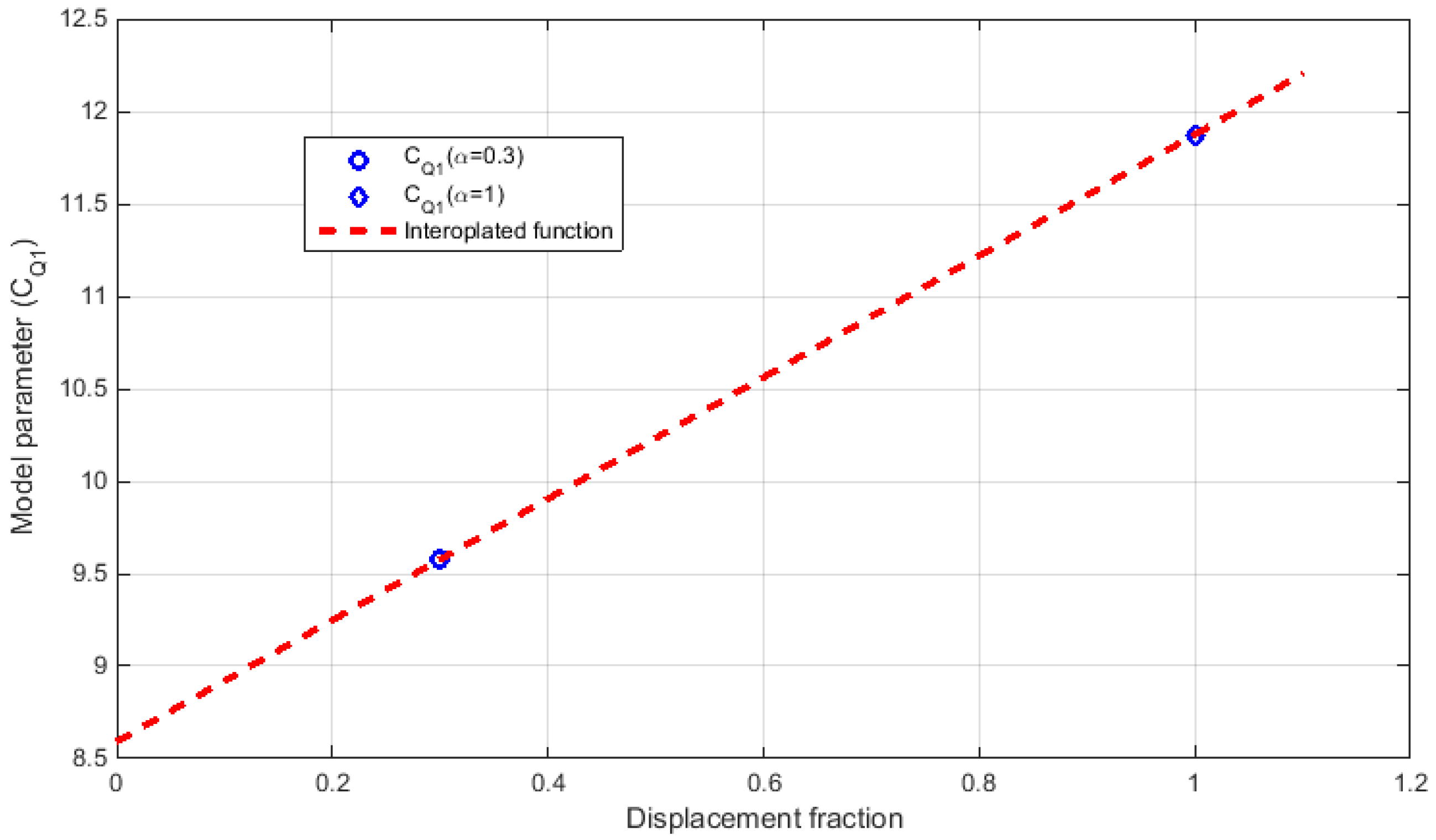
The linear least square fitting approach is used to identify the parameters of the models for each case, and once all the parameters for both cases are identified, coefficients can be expressed as a function of the displacement fraction ($\alpha$) using linear interpolation between the two coefficients, as shown in Figure 7 for the coefficient $C_{Q1}$. Linear interpolation is convenient to obtain the parameters of the loss model at different operating points, since manufacturers’ only provide the data for two operating points, but it should be noted that the real behaviour of the motor is not expected to be linear.

Since the manufacturers’ data is given in speed percentage, as shown in Figure 6a, the same model can be employed for different motor sizes by scaling the model as follows [21]:

$$Q_M^{RS}=\frac{D_{\omega }^{RS}}{D_{\omega }}\frac{{\omega }_{rated}^{RS}}{{\omega }_{reated}}{Q}_M\left(\frac{{\omega }_{rated}}{{\omega }_{reated}^{RS}}{\omega }_M,\Delta p_M\right),$$

(13)

$$T_M^{RS}=\frac{D_{\omega }^{RS}}{D_{\omega }}{T}_M\left(\frac{{\omega }_{rated}}{{\omega }_{rated}^{RS}}{\omega }_M,\Delta p_M\right),$$

(14)

where $D_{\omega }^{RS}$ is the displacement of the re-sized motor, and ${\omega }_{rated}$ and ${\omega }_{rated}^{RS}$ are the rated rotational speed of the baseline and re-sized motors, respectively.

Several types of hydraulic motors are currently available for diverse applications. Hydraulic motors that can rapidly vary the displacement are needed in WECs, due to the variability of the resource, so high efficiency is required not only at the optimum, but also at part-load operating conditions. Different hydraulic motor topologies are suggested in different hydraulic system configurations, e.g., a bent-axis hydraulic motor in [22] or a swash-plate motor in [21], for which the model structure presented in Equations (10)–(14) is suitable. However, similarly to the case of the hydraulic cylinder, it may be necessary to identify the model parameters for each specific case.

In the mathematical model presented in this paper, pressure losses in transmission lines are neglected, which is reasonable if short transmission lines are assumed.

3. Experimental Set-Up

In order to validate constant pressure and variable pressure circuits, it is necessary to use two separate test rigs. The particulars of these test rigs are discussed in this section, but there are a number of commonalities that it is prudent to document first.

Both test rigs were set-up on the same bed plate at the University of Bath’s Centre for Power Transmission and Motion Control (PTMC). Both rigs were driven by a double ended high precision linear actuator with 250 mm of stroke and piston area of 25 cm${}^2$. The linear actuator was operated in position control and was powered by a power pack capable of delivering 52 L/min at pressures up to 195 bar. A Simulink Real-Time system was used for data logging and control purposes in both test rigs, using a National Instruments PCI6221 data acquisition (DAQ) board sampling (Newbury, UK) at 1 kHz and a National Instruments PCI6229 DAQ board sampling at 100 Hz on the constant- and variable-pressure rigs, respectively.

Both test rigs were also constructed from discrete components and, as a result, losses within the circuits are higher than would be expected within custom manufactured units of similar design. Maximising efficiency was not the intent of these test rigs, and so these losses were not of concern, as long as they could be quantified for the purpose of model verification.

3.1. Constant-Pressure Configuration

The hydraulic circuit used for validating the constant pressure model varies from that shown in Figure 2 due to its use of an unequal area actuator. This necessitates further changes in order to maintain similar flow rates in extension and retraction with an area ratio of approximately 2:1. Figure 8 shows the modified PTO and

Table 1. Constant pressure test rig components.

No.	Description	Details
1	PTO cylinder	40 mm bore, 28 mm rod, 300 mm stroke
2	Regenerative check valves	0.35 bar preload
3	Rectification check valves	0.35 bar preload
4	HP accumulator	3.8 L, 10 bar precharge
5	Relief valve	100 bar cracking pressure
6	Gear motor	4.0 cc/rev
7	DC Generator	90 W at 3000 rpm
8	LP accumulator	1 L, 2 bar precharge
9	Boost pump	4 cc/rev, 7 bar relief pressure
10	Throttle valve	3/8" needle valve

details the individual components.

Hence, when the actuator is retracting, part of the fluid exiting the piston chamber (chamber A in Figure 8) is transferred, via the regenerative check valve ②, to the annulus chamber (chamber B in Figure 8). As a consequence, the rectified flow that goes to the accumulator 4 and, eventually, to the hydraulic motor 6, is equal to the annular area multiplied by the piston velocity (or half the piston area multiplied by piston velocity, due to the 2:1 area ratio). In contrast, when extending, the annulus flow is rectified to feed the motor and the LP accumulator and boost pump provide make-up flow to the piston chamber. A fixed-displacement motor was used in the PTO along with a DC generator, and a throttle valve was included in the circuit to mimic the variations of the hydraulic motor displacement.

In Figure 8, the location of the six pressure sensors and two flow sensors used in the experimental rig can be seen. The pressure sensors themselves were all Transinstrument 2000 series (Gems Sensors and Controls Ltd, Basingstoke, UK) rated to 250 bar and individually calibrated before installation. The flow meters were from the Hydac EVS3100 series (Sulzbach/Saar, Germany) capable of measuring flows between 6 L/min and 60 L/min and were delivered pre-calibrated and with signal conditioning. The physical location of these flow meters and the other major components are shown in Figure 9 .

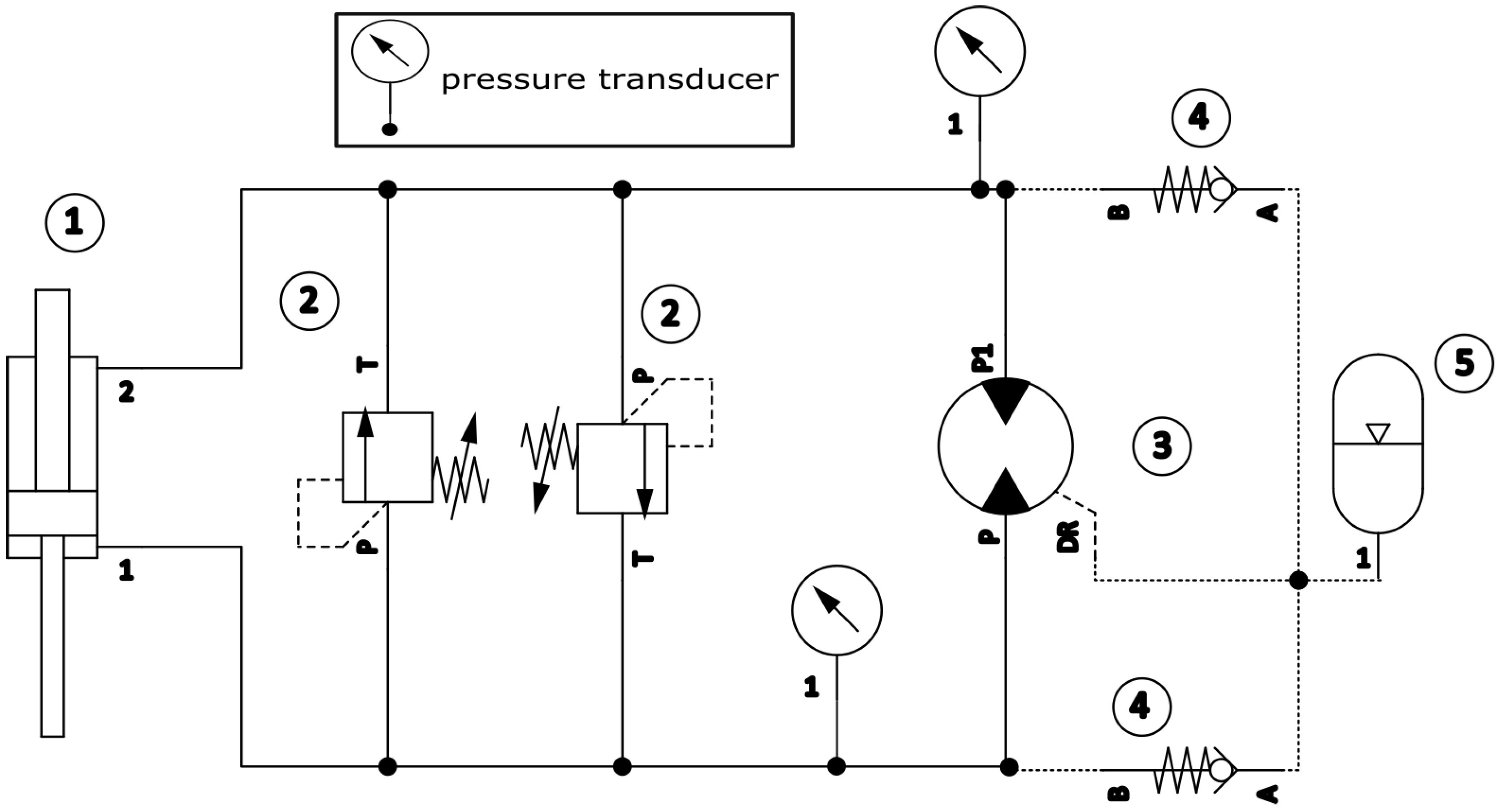
3.2. Variable-Pressure Configuration

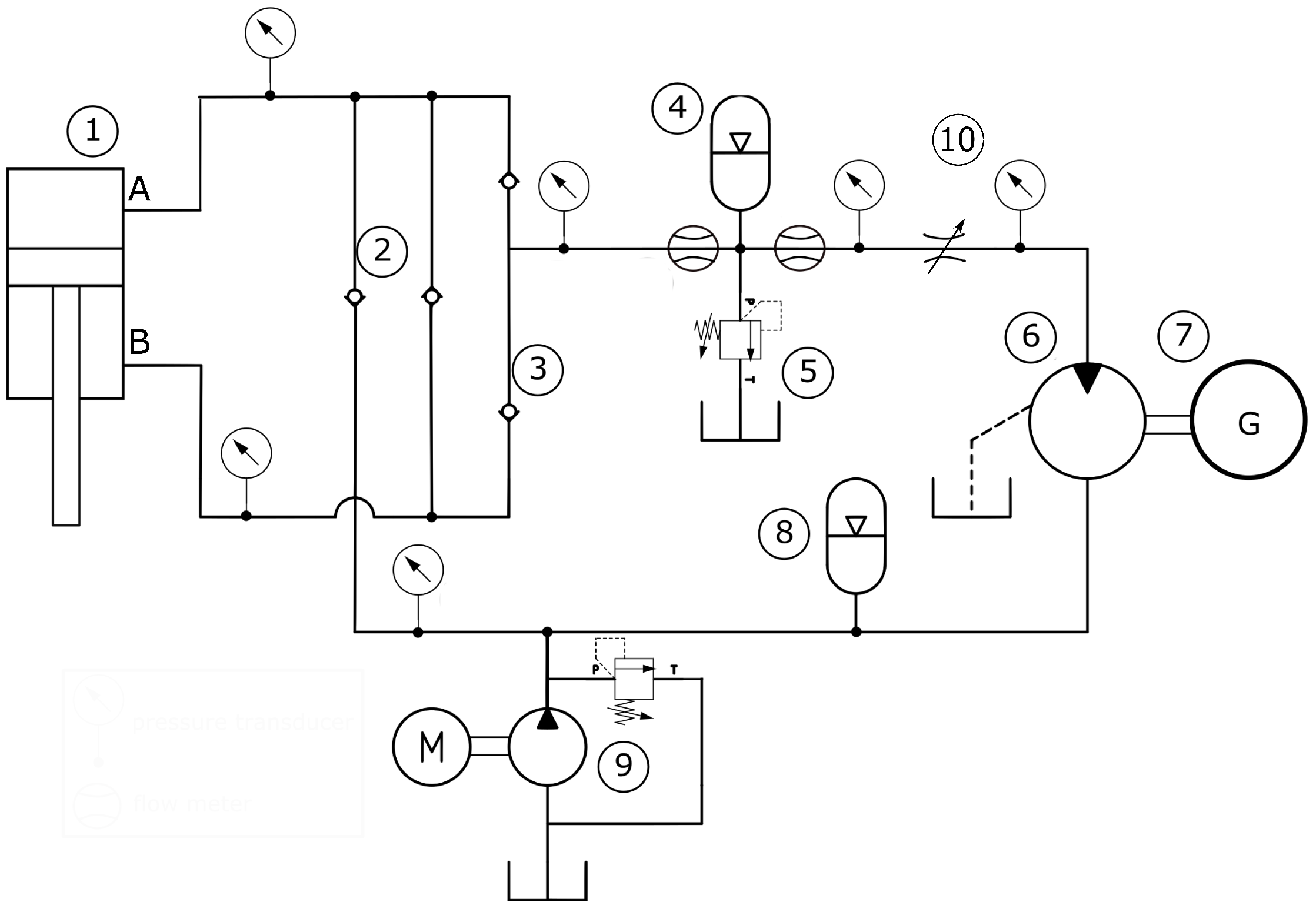
The hydraulic circuit used to validate the variable pressure configuration also used a fixed displacement motor, rather than the variable displacement motor shown in Figure 3. The leakage from the motor is directly returned to the circuit via an accumulator and a pair of check valves, obviating the need for a boost pump. Pressure signals are measured by means of pressure sensors from the Parker ASIC series (Cleveland, OH, USA) rated to 250 bar, which are calibrated at manufacture. Figure 10 shows the complete hydraulic circuit and

Table 2. Variable pressure test rig components.

No.	Description	Details
1	PTO cylinder	30 mm bore, 25 mm rod and 500 mm stroke
2	Relief valves	200 bar cracking pressure
3	Gear motor	7.8 cc/rev displacement
4	Leakage check	0.35 bar cracking pressure
5	Accumulator	5 L, 1 bar precharge

shows the details of each component.

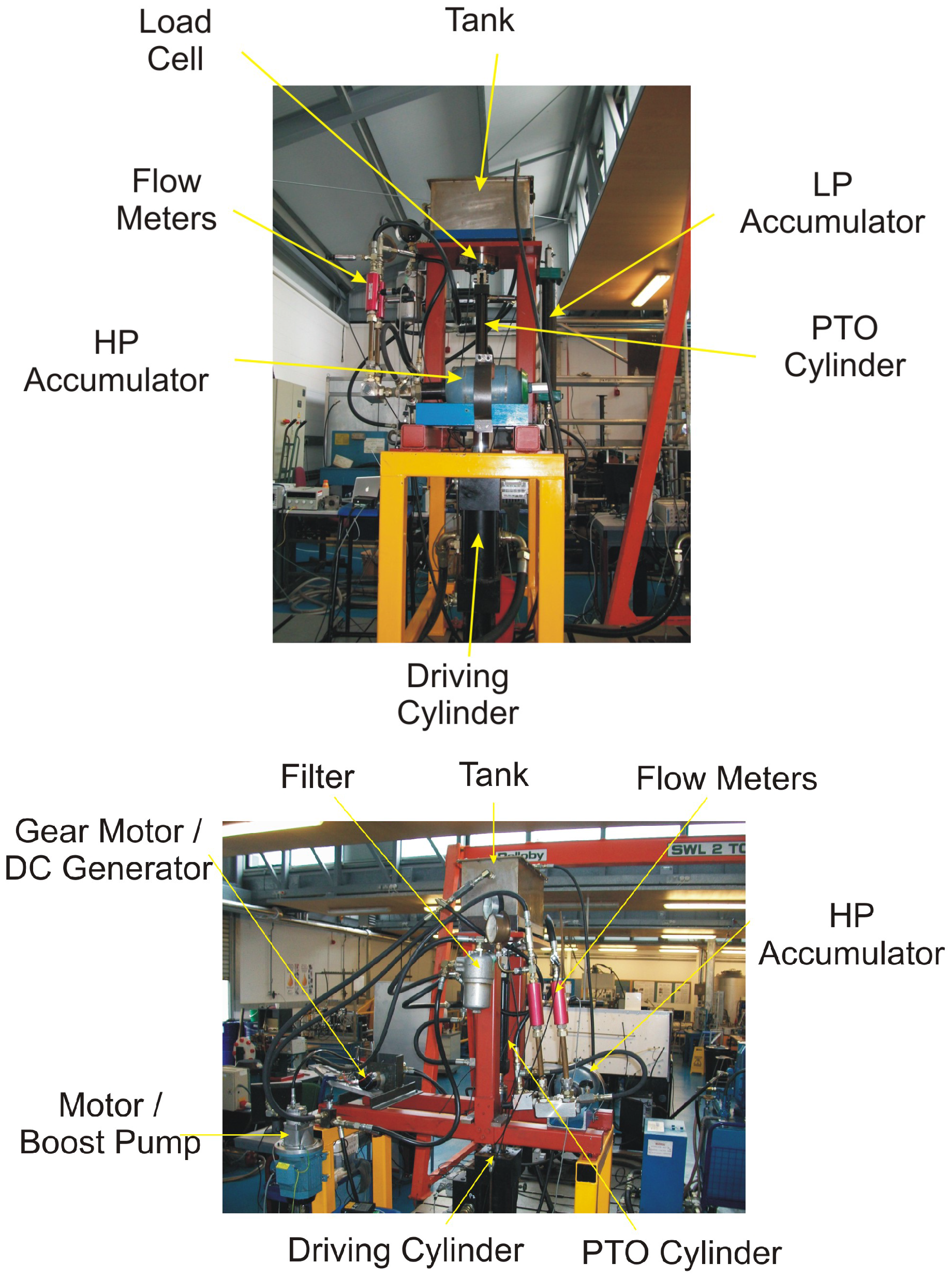
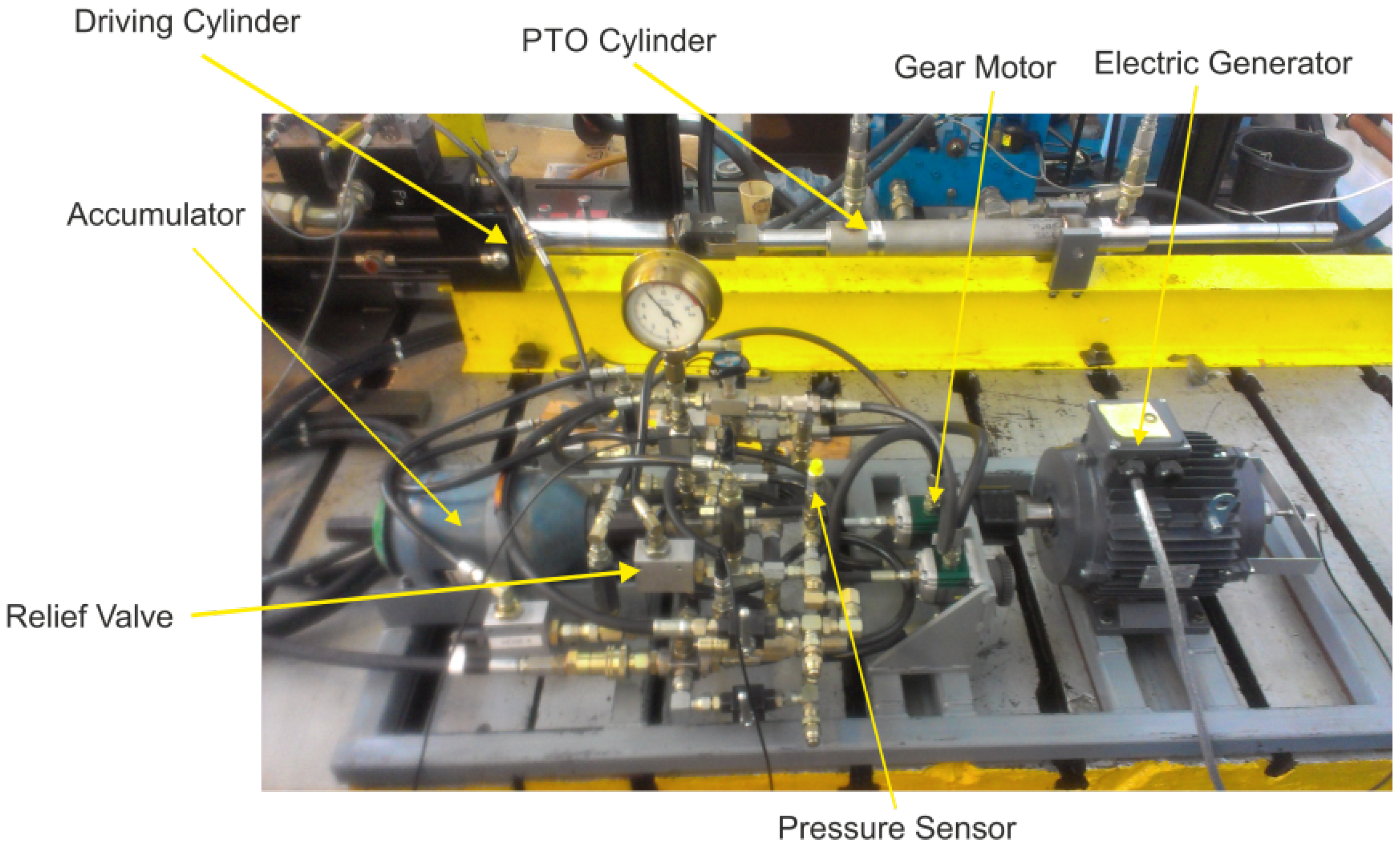
There are two motors shown in the Figure 11, as different sized motors were tested in the PTO. However, all results discussed in the present paper are measured with the 7.8 cc/rev motor installed.

3.3. Hydraulic Motor Model in AMESim

The validation of the hydraulic system was carried out using experimental results obtained in previous projects, for which the results of the hydraulic motor were not available. Therefore, resort to a high-fidelity hydraulic model was made to validate the mathematical model of the hydraulic motor, as mentioned in Section 1. A comparison is made between the model presented in Section 2.4, referred to as the Schlösser model in the following, and two different models created with the high-fidelity AMESim software, defined as idealised and detailed models.

AMESim is a physical modelling and simulation package for mechatronic systems based on bond graph methods. It is used widely within the fluid power industry and there are numerous publications validating its results against empirical data, including [39,40,41,42].

Both models created in AMESim reproduce the behaviour of a gear motor and use the pressure at the HP and LP accumulators, and the motor’s velocity of the numerical models, as inputs, and output the torque at the motor shaft and flow at the outlet of the hydraulic motor.

3.3.1. Idealised Model

The idealised motor assumes a perfect motor with no losses and continuous flow. Therefore, motor flow in the idealised model is a linear function of the shaft velocity used as input. It is further assumed that there were no losses between the pressure sensors and the motor. This is the simplest model of a hydraulic motor and is created as a reference for future models.

3.3.2. Detailed Model

A second model is also created, which models the individual teeth of the gear motor, and so has a displacement that varies with the absolute rotational position of the motor. The pumping gears have a total of 12 driving and 12 driven teeth with a module of 2.65 mm and width of 7 mm each. These dimensions input to the gear pump model and a contact angle of 20 assumed from the available literature.

This detailed motor model is coupled to a Wilson loss model, which uses the same efficiency map as shown in Figure 6, originally used to fit the hydraulic motor model developed in Section 2.4. The motor torque measured ignores the effect of inertia within the motor or generator, and so is more variable than would actually be seen at the motor shaft.

4. Validation

The two experimental set-ups described in Section 3 allow for a complete validation of the mathematical models, analysing the performance of the different components of the hydraulic PTO systems under different operating conditions.

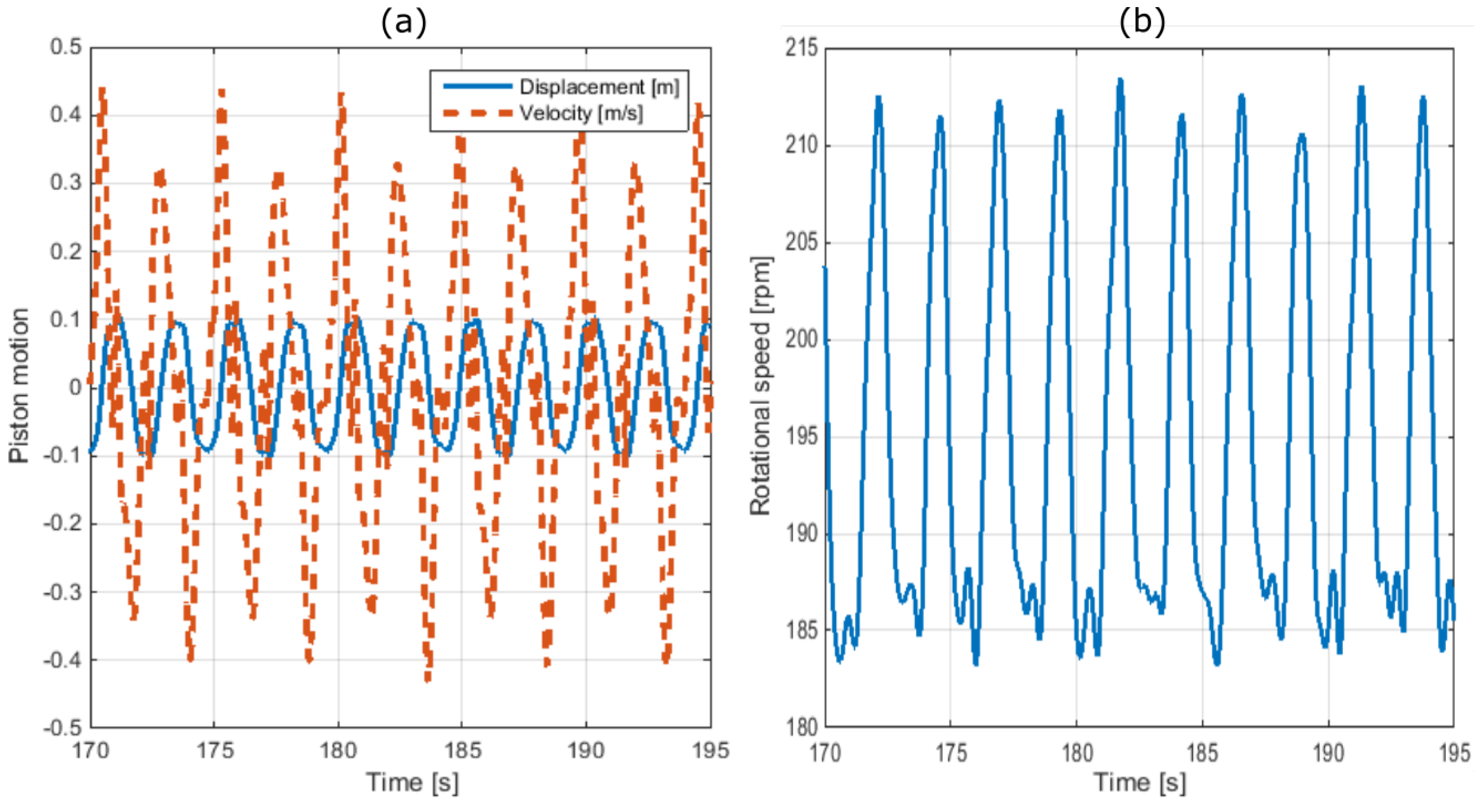
The inputs for the mathematical models are, for both hydraulic PTO configurations, piston position and velocity, and rotational speed of the electrical generator, as illustrated in Figure 1. Those inputs are taken directly from the experimental data and the outputs from the mathematical models are compared to the test-rig measurements and results from the high-fidelity software AMESim. Figure 12a shows the displacement and velocity of the piston and Figure 12b illustrates the rotational speed for one of the test cases simulated in the constant-pressure experimental set-up.

In the test-rig with the constant-pressure configuration, the experimental PTO was coupled to a hydrodynamic model that reproduces the behaviour of a WEC by means of a hardware-in-the-loop (HIL) system. In the experiments used for the validation in this paper, the WEC was a vertical cylinder of 2 m radius and 6 m draft, with an extended hemisphere in its lower end. More details about the WEC and the HIL system are given in [30]. Hence, the hydrodynamic model computes the position and velocity of the WEC (and, thus, postion and velocity of the piston in the hydraulic cylinder), which are used as inputs for the experimental PTO.

Three test cases, based on regular waves, were studied in the constant-pressure test rig:

• 10 s period and 1.5 m wave amplitude,
• 10 s period and 1 m wave amplitude, and
• 12 s period and 1.25 m wave amplitude,

which needed to be scaled down (using a scaling factor of 10) to be implemented in the experimental PTO. For the validation of the mathematical model with the constant-pressure configuration, the hydrodynamic model of the HIL system is ignored, since the mathematical model for the hydraulic PTO is isolated, and piston position and velocity are used as inputs.

In the case of the variable-pressure configuration, no HIL system was implemented, and piston position and velocity were used as inputs. A total of 20 test cases were analysed, combining four different sinusoidal input signals and five damping coefficients for the force control, implemented through the hydraulic motor.

Hydraulic cylinders and motors are the most important components of the hydraulic systems because the performance of the whole system essentially depends on the performance of these two components. The major challenge when modelling hydraulic cylinders is to accurately reproduce losses and dynamics due to friction. In the case of the hydraulic motor, friction and leakage losses are the main challenge.

Therefore, the validation of the mathematical models focuses on the two main components, carefully examining friction effects in hydraulic cylinders, and losses in hydraulic motors.

4.1. Hydraulic Cylinder

The performance of the hydraulic cylinder strongly depends on the system topology. In the case of constant-pressure configurations, the pressure in the cylinder chambers and, as a consequence, the force applied on the WEC, are practically constant, as illustrated in Figure 13 and Figure 14. In contrast, the pressure and force of the hydraulic cylinder in variable-pressure configurations follow the profile of the velocity, as shown in Figure 15 and Figure 16.

4.1.1. Constant-Pressure Configuration

Pressure in the hydraulic cylinder is driven by the pressure in the hydraulic accumulators, which, in turn, depends on the pre-charge pressure and the oil volume, as shown in Equation (8). The pressure of the oil in the accumulator sets the threshold for the check vales, so that check valves open only when pressure in the cylinder chamber is higher than in the HP accumulator.

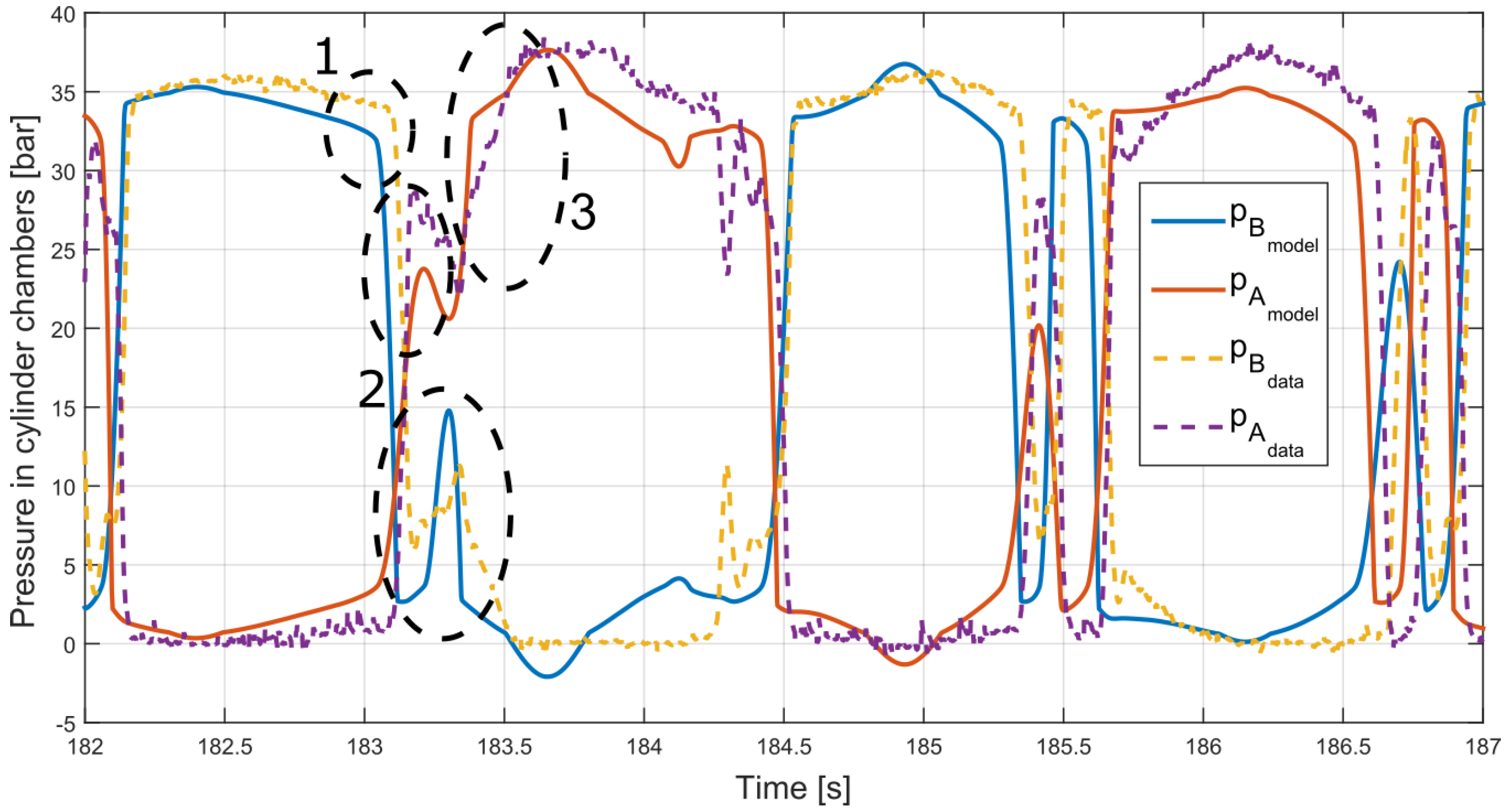
As one can note from Figure 13, the hydraulic cylinder in the constant-pressure configuration repeats the same cycle during the whole simulation. When the piston reaches its final position (1 in Figure 13), the pressure in the high-pressure chamber starts to reduce, falling below the accumulator pressure. At that point, check valves close and the piston starts to oscillate for a short period of time, which produces pressure fluctuations in both chambers (2 in Figure 13). As soon as the pressure in any of the chambers increases again over the pressure in the HP accumulator, check valves open again, and the piston starts to move ‘freely’, pushing the oil in the chamber, and, consequently, increasing the pressure in the chamber (3 in Figure 13). When the piston again reaches its end point, the whole process repeats in the other chamber.

The behaviour of the hydraulic cylinder in the constant-pressure configuration is similar for all the test cases analysed for the validation, where the profile of the pressure signals is practically identical and only the magnitude of the signals changes from one test case to another. Figure 13 illustrates the pressure in the chambers of the hydraulic cylinder for the 12 s period and 1.25 m amplitude test case, showing good agreement between the experimental results and the results from the mathematical model, in the sense that the profile and magnitude of the pressure signals are similar. However, the pressure signals appear to be slightly flatter at low pressures for the experimental results, while one can notice a negative overshoot for the results obtained from the mathematical model. In addition, the pressure drop across the check valves is shown to be larger for the experimental case and a phase lag exists between the experimental measurement and the numerical simulation as a result of the different pressure transitions, which are instantaneous in the mathematical model.

Similar agreement can be observed in Figure 14 for the piston force, where friction or inertia forces are also considered. The phase lag between the mathematical model and the experiments remains, as expected, in the force signals. However, it should be noted that the effect of friction is rather low in these test cases (about 1% of power loss due to friction based on the mathematical model).

4.1.2. Variable-Pressure Configuration

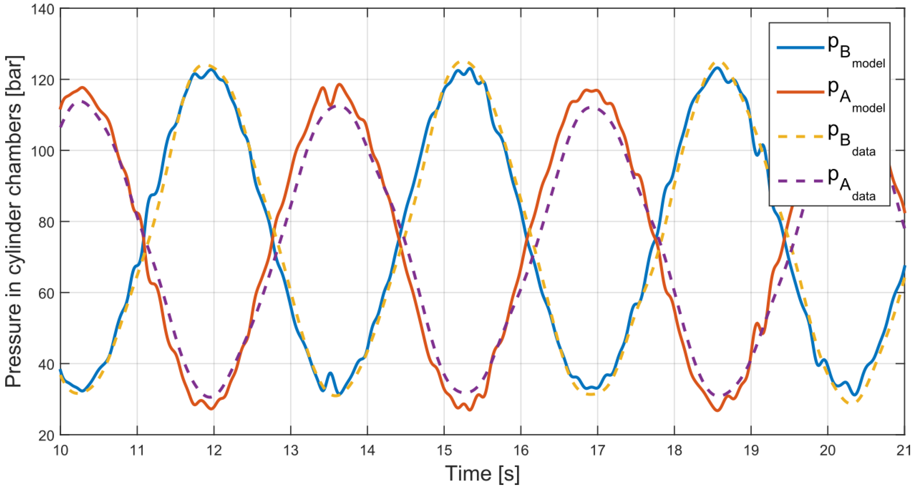
In the case of the variable pressure configuration, agreement between the experiments and the numerical simulations is also good for the different test cases, as illustrated in Figure 15, where the pressure signal is clearly asymmetric. This asymmetry appears due to a non-symmetrical control force signal, with a different damping coefficient for each direction of motion.

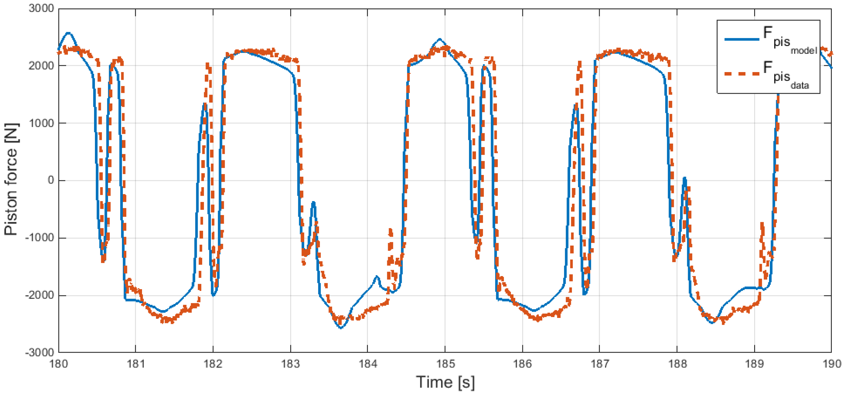
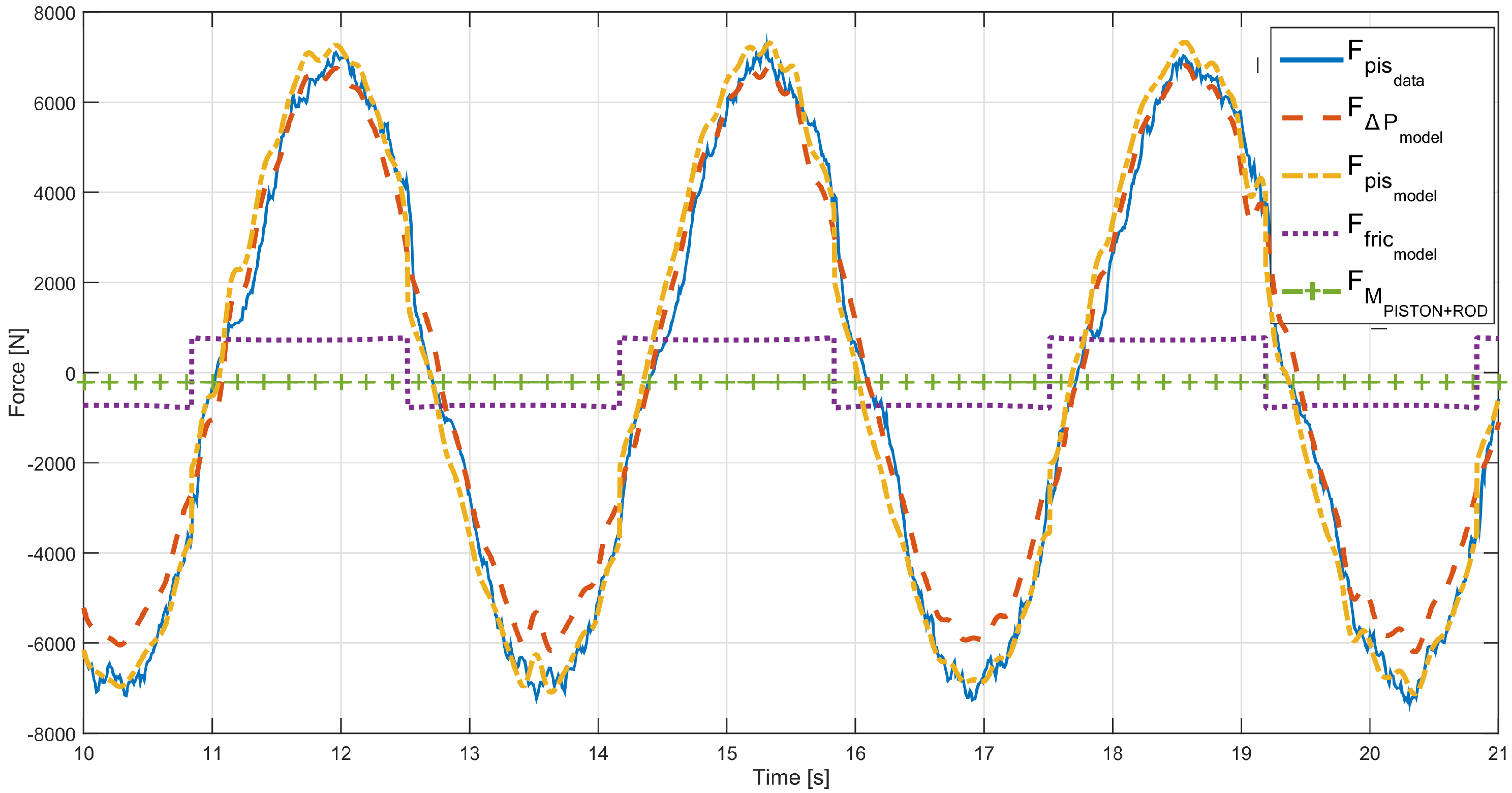
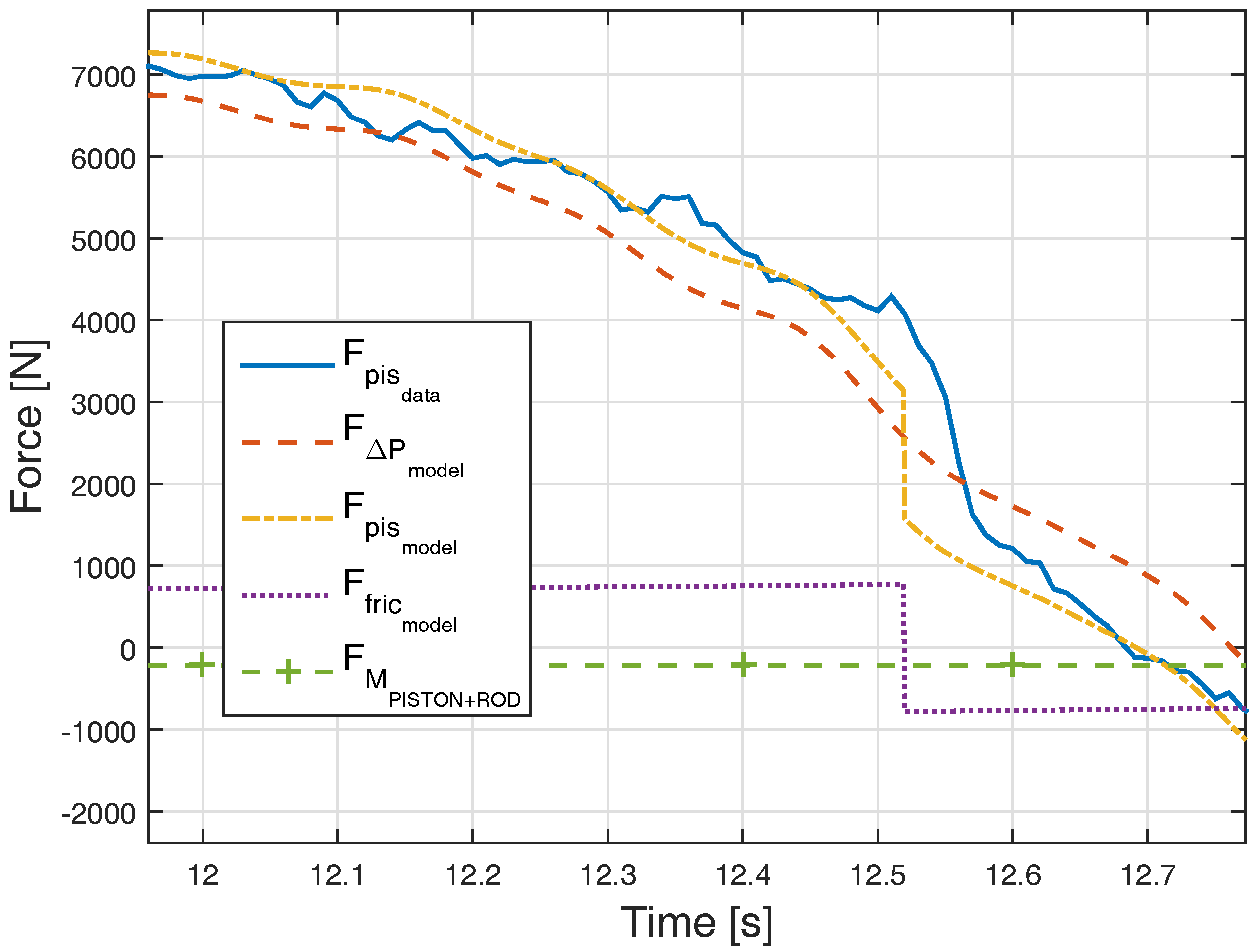
Similarly to the constant-pressure configuration, measured and simulated force signals match accurately, as illustrated in Figure 16. Apart from the total force signal, Figure 16 also shows the contributions of the different factors, such as pressure difference, friction or piston mass.

Hence, one can observe that, for the pressure force, referred to as the force considering only the contribution of the pressure difference in the cylinder ($F_{\Delta P_{model}}$), the amplitude is lower than the experimental piston force ($F_{pi{s}_{data}}$). In addition, pressure force is, as expected, asymmetric, while experimental piston force appears to be completely symmetric. However, when friction force and gravity force due to the piston mass are added to the pressure force, the total piston force obtained from the mathematical model ($F_{pi{s}_{model}}$) accurately matches the experimental piston force.

Finally, the friction force signal shows the relevance of the Coulomb and static friction over the viscous friction and, as a consequence, the impact of the friction force is especially recognisable at low velocity. When friction force suddenly changes from positive to negative, or vice versa, force signal also shows an abrupt change, which can only be reproduced by accurately modelling friction. Figure 17 illustrates the impact of the friction force at low velocity, where the force signal considering the pressure difference alone simply follows the velocity profile, while the signal that includes friction clearly shows an abrupt drop, similarly to the measured force signal.

4.2. Hydraulic Motor

Losses in the hydraulic motor also depend on the characteristics of the operation, especially pressure difference and rotational speed, as described in the Schlösser model defined in Equations (11) and (12).

The well-known simulation software, AMESim, is employed to accurately model the performance of the hydraulic motor, as described in Section 3.3. Hence, pressure results from the numerical model described in Section 2 are used as inputs for the hydraulic motor model created in AMESim to validate the Schlösser model developed in Section 2.4.

Thus, flow and torque in the hydraulic motor are analysed, comparing the results from the mathematical model described in Section 2.4.1, referred to as the Schlösser model in the following paragraphs, to the results obtained from the AMESim models.

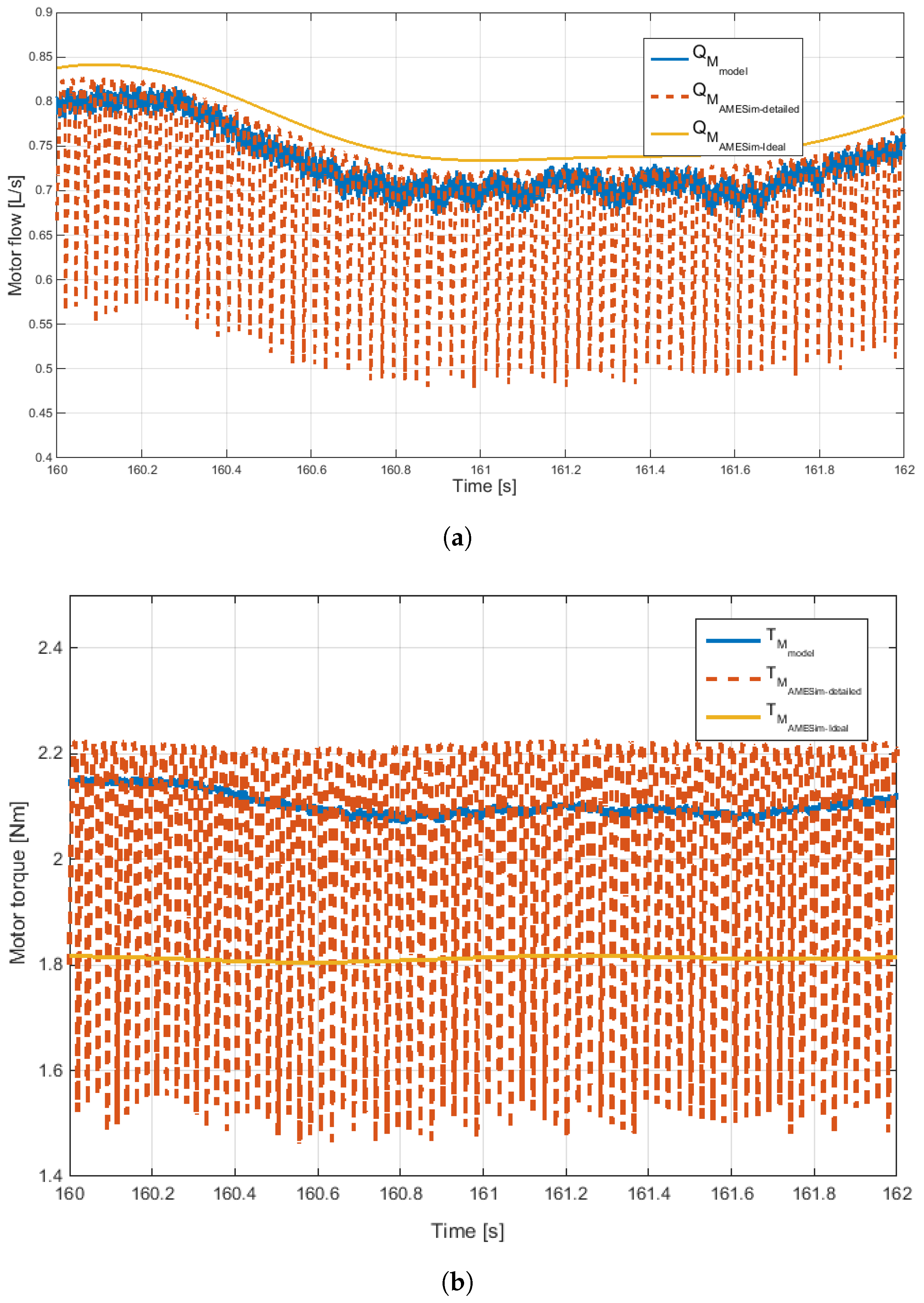
Figure 18a,b illustrate the motor flow and torque, respectively, where the flow of the Schlösser model stays always below the ideal flow, due to the losses neglected in the ideal AMESim model, and the torque stays always above, to overcome the friction losses and supply the required torque. Compared to the detailed AMESim model, the flow and torque of the Schlösser model appear to follow the upper envelope of the flow and torque, which suggests that the efficiency is similar for the detailed AMESim and Schlösser models. However, significantly more variations can be observed in the detailed AMESim model, due to the modelling of the movement of the individual pumping elements, which cannot be captured unless a detailed model is used.

5. Conclusions

The present paper validates the mathematical models for hydraulic transmission systems used in the power take-off of wave energy converters. The different topologies suggested in the literature are divided into two main configurations, depending on the operational characteristics, as described in Section 1.1: constant-pressure and variable-pressure configurations. The mathematical equations to model the different components used in the two configurations are given in Section 2, including the main nonlinear dynamics and losses, such as friction in hydraulic cylinders or losses in the hydraulic motor.

Two experimental set-ups described in Section 3, including a set-up that reproduces the characteristics of a constant-pressure configuration and another set-up that emulates the variable-pressure configuration, are employed in the validation. That way, the validation covers the different possibilities of using hydraulic transmission systems in wave energy. In addition, a well-known software for hydraulic systems, AMESim, is used to validate the performance of the hydraulic motor. Results from the mathematical model and the experiments are compared in Section 4, which mainly focus on the performance of the hydraulic cylinder and motor.

Results of the hydraulic cylinder show very good agreement for pressure and force values in the different test cases analysed for the two configurations. In the constant-pressure configuration, the effect of the rectification valves is well reproduced by the mathematical model, including the pressure and force oscillations that arise when the piston approaches its final position. In addition, the mathematical model shows the ability to capture the asymmetry observed in the variable-pressure configuration experiments and demonstrates the effectiveness of the friction model, reproducing the effect of the static friction at low velocities.

The Schlösser model for the hydraulic motor is shown to be more realistic than the ideal model implemented in AMESim, while the efficiency of the Schlösser model appears to be similar to the detailed AMESim model, although the detailed AMESim model includes other effects, such as wave propagation that cause larger variations in the flow and torque.