Performance Characteristics of a 4 × 6 Oil-Free Twin-Screw Compressor

Abstract

The screw compressor in the early stage of development is generally known as the oil-injection type. However, escalating environmental problems and advances in electronic components have spurred continuous R & D to minimize the oil content in compressed air. The oil-free twin-screw compressor is continuously compressed by inner volumetric change between rotors and casing. For this reason, in order to predict the overall performance of the screw compressor at the early stage of the design process, industry still relies on the empirical method. However, it is difficult using the existing empirical method to gain more information of the inner fluid flow of the twin-screw compressor. Flow simulation techniques using CFD are required. This study presents applications of a recently proposed overset grid method to the solution of the flow around a moving boundary. In order to analyze the performance of a 4 × 6 oil-free screw compressor, the 3-D, unsteady and compressible flow fields were numerically calculated with a shear stress transport (SST) turbulence model, and implemented by the commercial software, Star-CCM+. The pressure distributions were calculated and graphically depicted. Results also showed that the volumetric and adiabatic efficiencies of the screw compressor measured by the experiments were 78% and 71%, respectively.

1. Introduction

A screw compressor is provided with a male rotor and female rotor, which intermesh with each other when they rotate. These screw rotors are asymmetrical in their contour, and usually have quite complicated profiles. The purpose of gear tooth development is to improve the performance of the screw compressor. Generally, the profile efficiency is measured by a number of factors, such as low contact force, smooth torque transfer, short meshing line length, and large cavity volume. In terms of efficiency, the rotor profile influences the performance of the screw compressor. To be brief, in order to improve the performance of the screw compressor, a designer is faced with various problems. For example, the main geometrical parameters for improving the operating efficiency of the screw rotor are the area between the rotors, the gap tolerance between the rotor and the housing, the sealing line length, and the blow-hole area, which area it is recommended to reduce. Several researchers have continuously studied rotor profile design to improve the performance of the screw compressor.

In the mid-1980s, the A type of rotor profiles proposed by the Swedish company SRM became the standard for the industry, and research on the screw rotor profiles then began in earnest. Stosic and Hanjalic [1] proposed a general method for screw rotor profile generation. The rack-based profile generation method that they proposed contains all the elements of the modern screw rotor profile. There are limits for any commercial application, but it features a basis for further refinement and optimization. They observe that the main advantage of this method is its simplicity, which enables a variety of profiles to be created in a short time by practical rotor designers.

Tang and Fleming introduced a method to optimize the geometrical parameters for a refrigeration twin-screw compressor [2]. In order to optimize the geometrical parameters, such as the smallest blow hole area, the shortest contact line length per lobe, and the correct discharge port position suitable for a given discharge pressure, they developed a simulation program for the geometric calculation procedure, and to simulate the working process.

Stosic [3] proposed the envelope gearing method that is used to derive a meshing condition for crossed helical gears, and then used it to create the profile of a hobbing tool. The author applied the envelope theory of gearing as the meshing requirement for crossed helical gears. He showed that it was able to create a helical gear of the full meshing condition to the hobbing tool.

Stosic et al. [4] discussed some optimization issues of the rotor profile and compressor parts, using a 5 × 6 screw rotor profile. The adopted method was based on a rack generation algorithm for the screw rotor profile, combined with a numerical model of the compressor parts. Their designed compressor demonstrated higher delivery and better efficiencies than those using traditional approaches.

Most of the researches related to the screw rotor profile are concerned with predicting the effect on the performance of the screw compressor with respect to changes in the design variables, such as clearance, meshing line length, and rotor diameter and speeds. In view of the fact that the rotor profile has great influence on the efficiency of the screw compressor, researchers have attempted to develop a new method to generate the profiles that give the rotors of the compressor the optimum working efficiency. Stosic et al. [5] developed a comprehensive software package that included almost every aspect of thermodynamic and geometric modeling, and the capacity to transmit derived output directly into the CAD drawing system.

As for the operation characteristics of a gear compressor, time-dependent analysis is important in the internal compression stroke. This means that the boundary of the flow analysis area is changed during the calculation process. Therefore, when the gear rotates, the gear surface has a very complicated movement, which is becoming an important problem in CFD analysis. Several studies have been carried out with various attempts to find a breakthrough for CFD analysis.

Kovacevic [6] proposed some aspects of the so called SCORG advanced grid generation method with an algebraic method that features boundary adaptation and transfinite interpolation used in CFD, so as to increase the accuracy of the flow prediction. In this way, it has been shown that the performance of a screw compressor can be improved.

Voorde et al. [7] proposed a grid manipulator based on the ALE method. It is a time-dependent grid generation method that computes grid motions with local flow velocity in a stationary computational grid in a mixed form of Lagrangian and Eulerian methods. They showed that the compressible flow analysis calculation of a gear compressor is possible.

Rane et al. [8] described the advantages of the algebraic grid by comparing the two methods for generating custom grids described above, i.e., algebraic grid generation and differential decomposition methods. Also they showed that newly developed grid approach can maintain a complete hexahedral cell topology for grid generation at non-conformal boundaries.

The finite volume method is a powerful CFD numerical technique that allows fast and accurate solution for fluid flow within complex geometries; however, an acceptable grid system that describes shapes accurately must be available, in order for the method to be used [9].

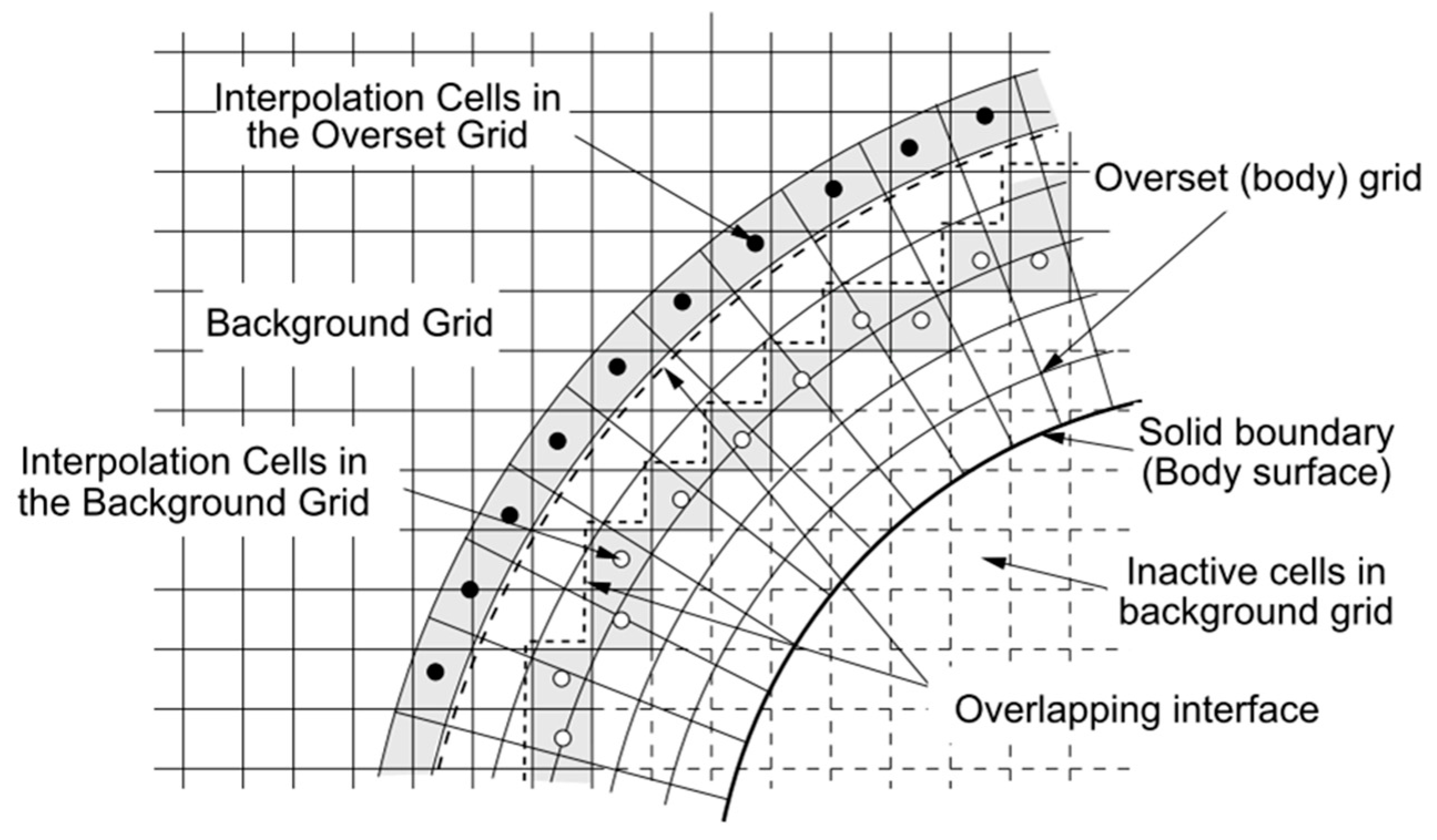
The aforementioned grid adjustment approach requires that the grids around the moving object could be transformed and regenerated to a new position at each time step. The flow solver can be easily conserved and the grids can be generated in domain conformal grid with one or several grid blocks to reduce the number of grids. However, this approach is not easy to interpolate the flow variables from old grid to new one at each time step. In addition, excessive processing and extra costs are required for grid generation. On the other hand, the overlapping grid method is based on the assumption that the grid components related to a complex and moving bodies are still in a stationary state, and the sub-grid components are superimposed on each other to define a relative motion by an arbitrary method. Among other two techniques, the overlapping grid approach offers more flexibility and the grid quality can be ensured. In this study, the CFD analysis of screw compressors was performed using the overlapping grid approach, which has been studied by many authors in recent years.

Steger and Benek [10] briefly reviewed some of the composite grid approaches used in aerodynamic applications. Li et al. [11] reported that the CFD prediction using dynamic overset CFD simulations consistently matched by extensive comparisons with experimental data for NREL VI wind turbine. Suman et al. [12] carried out the unsteady analysis for the SSE using the overlapping grid method. Although the information of the computed variables is lost at the grid interfaces, the meshing strategy such as the overlapping grid method can be applied to the complicated machine such as SSE from the previous studies.

The objective of this study was to determine the flow characteristics through CFD application of the screw compressor having a positive displacement process. In addition, this study describes the theory of screw rotor tooth profile generation and compares the CFD analysis results with the experimental results.

2. Theoretical Background

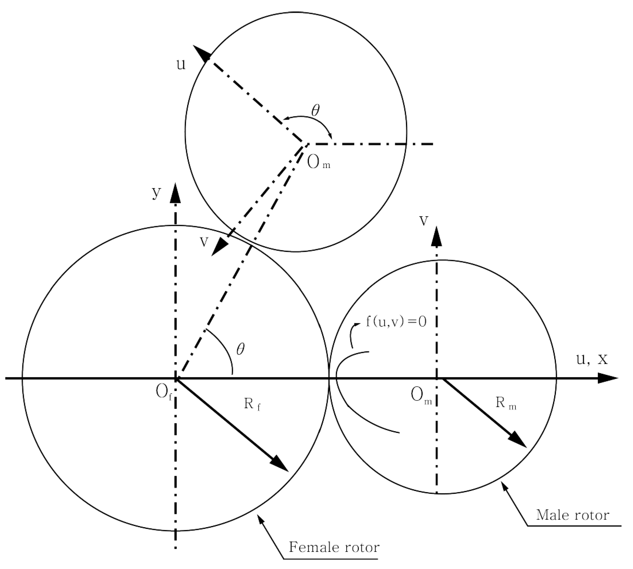
A screw rotor profile usually contains various kinds of functions, and it consists of mostly circular, cycloid, and arc curves. Figure 1 shows a male rotor rotated around a female rotor in the x-y coordinate system, which is fixed to the female rotor, while the u-v coordinate system is fixed to the male rotor. When the male rotor rotates by φ around the female rotor, the male rotor is rotated by θ$\left(\theta =\frac{R_f+R_m}{R_m}\phi \right)$ in the x-y plane. Therefore, the conversion formula of the x-y and u-v coordinate systems is defined in Equation (1) [13,14]:

$$\left[\begin{array}{c}x\\ y\end{array}\right]=\left[\begin{array}{c}\left(R_f+R_m\right)\cos \phi \\ \left(R_f+R_m\right)\sin \phi \end{array}\right]+\left[\begin{array}{cc}\cos \theta & -\sin \theta \\ \sin \theta & \cos \theta \end{array}\right]\left[\begin{array}{c}u\\ v\end{array}\right]$$

(1)

If the rotor profile curve of the driving rotor can be defined from the relation function of Equation (1), a rotor profile of the dependent rotor could be produced that satisfies a pair of meshing conditions.

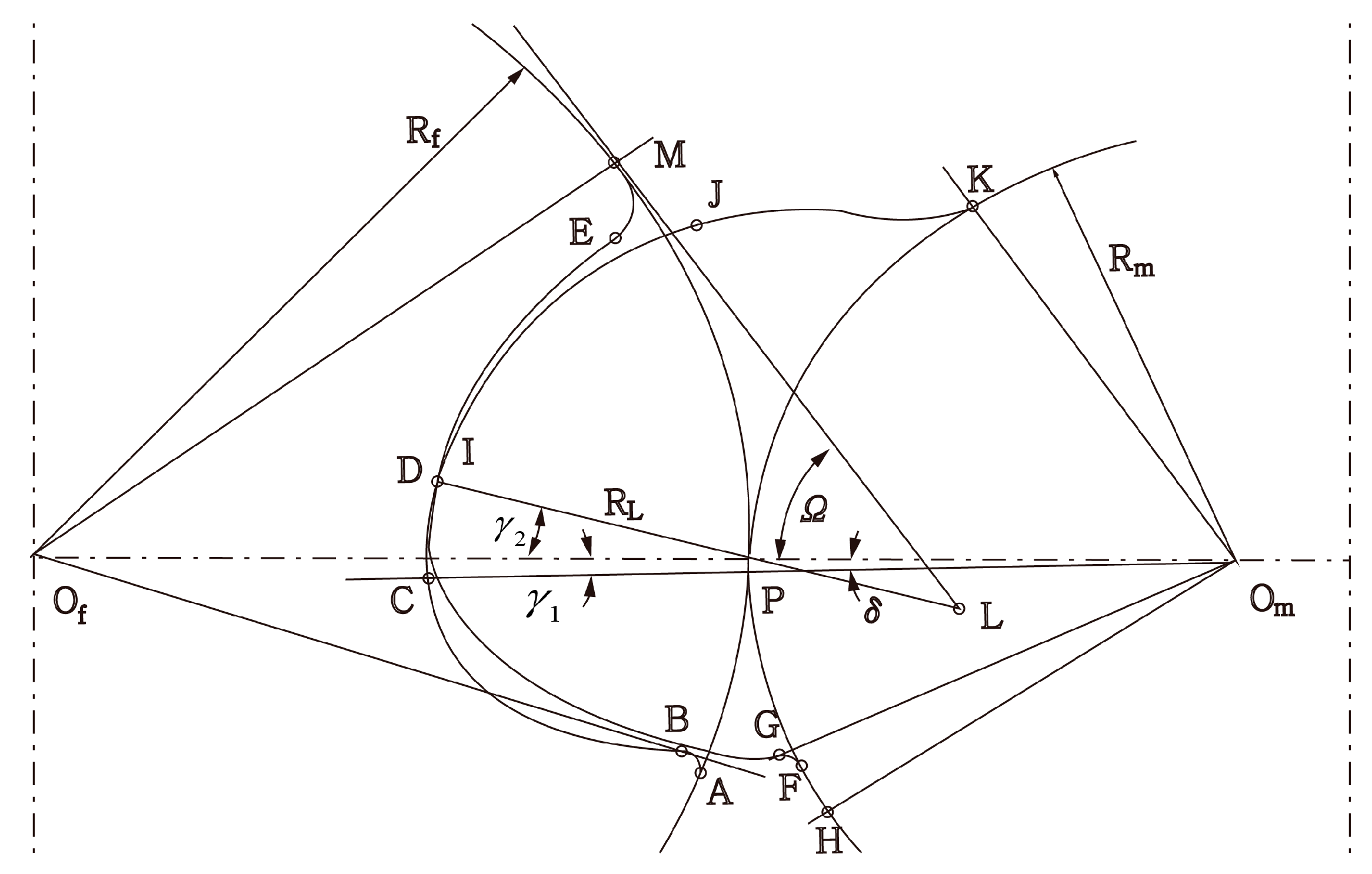
Figure 2 shows the location of arbitrary points on the dependent rotor profile in contact with the drive rotor. The driving rotor as a basis in the profile generation method is the female rotor, and the dependent rotor that is generated by the envelope function is the male rotor. The line that is used to generate the rotor profile is composed of an epi-trochoid, epi-cycloid, and a circular arc connecting each position.

Table 1. Curve form by point location.

No.	Female Rotor	Male Rotor
1	A–B: circular arc	F–G: generated by A–B
2	B–C: Epi-trochoid	G–H: Epi-cycloid by B–C
3	C–D: circular arc	H–I: circular arc
4	D–E: circular arc	I–J: generated by D–E
5	E–M: circular arc	J–K: generated by E–M

shows the shape of the curve for each position of the male and female rotors, of which the following equations are defined [15].

A–B: Insert the circular arc of radius r_s after the selection of the center position of point C so as to satisfy the continuous condition at points A and B.

B–C: The trajectory of a trochoid curve at point H, when the center O_m of the circle is rotated around the center O_f of the circle:

$$\begin{array}{l}x=C_d\cos \theta -O_{m}H\cos \left(\frac{C_d}{R_m}+\mathrm{\Omega }\right)\\ y=C_d\sin \theta -O_{m}H\sin \left(\frac{C_d}{R_m}+\mathrm{\Omega }\right)\\ \mathrm{\Omega }={\sin }^{-1}\left(\frac{R}{R_{io}}\sin \left({\gamma }_1\right)\right)\end{array}$$

(2)

C–D: The arc of the radius R centered on the pitch point P:

$$\begin{array}{l}\left\{\begin{array}{l}{C}_x\\ C_y\end{array}\right\}=\left\{\begin{array}{l}{R}_f-R\cos ({\gamma }_2)\\ R\sin ({\gamma }_2)\end{array}\right\}\\ \left\{\begin{array}{l}{D}_x\\ D_y\end{array}\right\}=\left\{\begin{array}{l}{R}_f-R\cos ({\gamma }_1)\\ R\sin ({\gamma }_1)\end{array}\right\}\end{array}$$

(3)

D–E: The radius R_L of the circular arc centered on the point L, where the location is the intersection of the tangent line of the arc on point M and of the extension line in the D–P:

$$\left\{\begin{array}{c}{L}_x=R_f+\delta \cos \left({\gamma }_2\right)\\ L_y=-\delta \sin \left({\gamma }_2\right)\end{array}\right\}$$

(4)

where:

$$\delta =\frac{R^2}{2\left(R_f\cos \left({\gamma }_2\right)-R\right)}$$

(5)

E–M: The circular arc of the radius R_s, satisfying the continuity of point C in points M and B:

$$\begin{array}{l}\left\{\begin{array}{l}{N}_x\\ N_y\end{array}\right\}=\left\{\begin{array}{l}(R_f-R_s)\cos ({\theta }_1)\\ (R_f-R_s)\sin ({\theta }_1)\end{array}\right\}\\ \left\{\begin{array}{l}{M}_x\\ M_y\end{array}\right\}=\left\{\begin{array}{l}{R}_f\cos ({\theta }_1)\\ R_f\sin ({\theta }_1)\end{array}\right\}\\ \left\{\begin{array}{l}{E}_x\\ E_y\end{array}\right\}=\left\{\begin{array}{l}-(R+\delta )\cos ({\theta }_2)+L_x\\ (R+\delta )\sin ({\theta }_2)+L_x\end{array}\right\}\end{array}$$

(6)

$$\begin{array}{l}{\theta }_1={\sin }^{-1}\left(\frac{(R+\delta +R_s)\sin ({\theta }_2)+L_y}{R_f-R_s}\right)\\ {\theta }_2={\cos }^{-1}\left(\frac{{\left(R+\delta +R_s\right)}^2+\left(L_x{}^2+L_y{}^2\right)-{\left(R_f-R_s\right)}^2}{2\left(R+\delta +R_s\right)\sqrt{L_x{}^2+L_y{}^2}}\right)-{\theta }_3\\ {\theta }_3={\tan }^{-1}\left(\frac{L_y}{L_x}\right)\end{array}$$

(7)

Table 1 shows that the profile curves of the male rotor as a dependent rotor are generated by curves of the same contact trajectory with circular arc that is generated by the equations to the A–M. The male rotor was composed of circular arc with the same contact trajectory as each section of the female rotor described above.

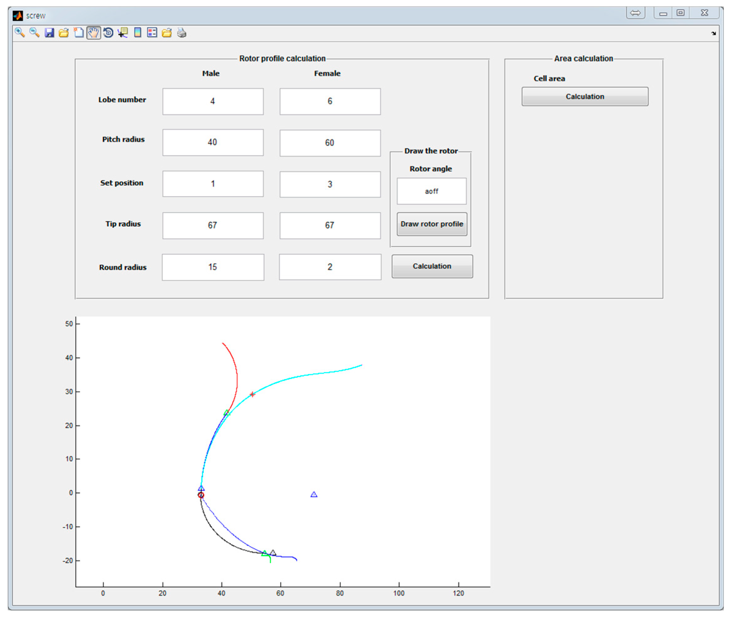
In this study, a MATLAB (Matlab 2015a, The MathWorks, Inc. Company: Natick, MA, USA) based tool design program was developed so as to easily obtain the curves equations from the design variables of various sizes and combinations required by the designer. Figure 3 shows the MATLAB-based program that can be used to calculate the screw rotor profile through the basic input variables. The basic input variables for rotor profile calculation are the number of lobe combinations, rotor radius, lobe end radius, and lobe width.

3. Numerical Method

3.1. Governing Equations

The mass or continuity conservation equation states that the rate of change of the mass inside a control volume V is equal to the difference between inflow and outflow mass fluxes across the volume surface S:

$$\frac{\partial }{\partial t}{\displaystyle \underset{V}{\int }\rho dV+{\displaystyle \underset{S}{\int }\rho \upsilon \cdot ds=0}}$$

(8)

where, ρ is the fluid density, and v is the working fluid velocity.

The conservation equation for momentum states that the total variation of momentum is represented by the time variation of momentum within the control volume, and transfer of momentum across the boundary of the control volume by fluid motion. This is caused by the net force acting on the fluid in the control volume:

$$\frac{\partial }{\partial t}{\displaystyle \underset{V}{\int }\rho \mathrm{v}dV}+{\displaystyle \underset{S}{\int }\rho \mathrm{vv}\cdot ds}={\displaystyle \underset{S}{\int }\sigma \cdot ds}+{\displaystyle \underset{V}{\int }\rho {\mathrm{f}}_{b}dV}$$

(9)

where, σ is the stress tensor representing the surface forces, and f_b represents the vector of body forces acting on the fluid.

$$\frac{\partial }{\partial t}{\displaystyle \underset{V}{\int }\rho hdV}+{\displaystyle \underset{S}{\int }\rho h\mathrm{v}\cdot ds}={\displaystyle \underset{S}{\int }q\cdot ds}+{\displaystyle \underset{V}{\int }\left(\sigma :\nabla {\mathrm{v}+\mathrm{q}}_T\right)dV}$$

(10)

where, h is the specific enthalpy, q is the heat flux vector, and q_T is the heat source or sink. If the fluid is considered to be thermally perfect, specific enthalpy depends only on temperature, via the following relation:

$$h=c_{p}T$$

(11)

where, c_p is the specific heat at constant pressure, and T is the temperature.

The generic transport equations to obtain the discrete counterpart of above all the governing equations are as follows:

$$\underset{\mathrm{Rate}\mathrm{of}\mathrm{change}}{\underbrace{\frac{\partial }{\partial t}{\displaystyle \underset{\mathrm{\Delta }V}{\overset{}{\int }}\rho \varphi dV}}}+\underset{\mathrm{Convection}}{\underbrace{{\displaystyle \sum _{j=1}^N{\displaystyle \underset{S_j}{\overset{}{\int }}\rho \varphi \mathrm{v}\cdot \mathrm{ds}}}}}=\underset{\mathrm{Diffusion}}{\underbrace{{\displaystyle \sum _{j=1}^N{\displaystyle \underset{S_j}{\overset{}{\int }}{\mathrm{\Gamma }}_{\varphi }\nabla \varphi \cdot \mathrm{ds}}}}}+\underset{\mathrm{Surfacesource}}{\underbrace{{\displaystyle \sum _{j=1}^N{\displaystyle \underset{S_j}{\overset{}{\int }}{\mathrm{q}}_{\varphi s}\cdot \mathrm{ds}}}}}+\underset{\mathrm{Volumesource}}{\underbrace{{\displaystyle \underset{\mathrm{\Delta }V}{\overset{}{\int }}{q}_{\varphi V}dV}}}$$

(12)

where, the surface integrals in Equation (12) are here represented as a sum of integrals over a number of cell faces defining the cell, $P_0$. The equation consists of the rate of change (steady or unsteady term), convection, diffusion and source terms.

In this study, we adopt a local time derivative approach to calculate the flow field for a moving grid by solving the above equation for a stationary grid. In order to approximate the unsteady term, it is necessary to use the variable values from one or two previous time steps. Therefore, these values can be obtained by interpolation. The following equation shows the linear interpolation to obtain the old value from the new CV center:

$${\varphi }_{P_0^{new}}^{old}={\varphi }_{P_0^{old}}^{old}+{\left(\nabla \varphi \right)}_{P_0^{old}}^{old}\cdot \left({\mathrm{r}}_{P_0^{new}}-{\mathrm{r}}_{P_0^{old}}\right)$$

(13)

3.2. Grid Systems and Model Setting

The overlapping grid technique is the so-called chimera grid. This grid technique has been developed by researchers in the past. In these methods, the computational domain is composed of grids that overlap with each other according to any method. The advantage of such a grid arrangement is that it is possible to employ higher quality grids than when dealing with complex geometric shapes. Figure 4 shows some definitions and the notation for a detailed view of the overlapping grid system. Here, one representing portion as “○” indicates the node points of the adjacent cells to the arbitrary boundary in the background grids [16]. The cells in the overlapping grid are divided into three groups: active (discretization), interpolation, and inactive (hole) cells. The solutions are obtained from grid systems that are constructed independently of each other, and the continuity of solutions is obtained by interpolating information between the grids.

In this study, numerical analysis is performed using the overlapping grid technique, which is flexible and capable of multiple continuous discretization in complex geometric shapes and dynamic body problems. The finite volume method (FVM) is adopted to solve the governing equations described above. The three-dimensional compressible flow fields through the rotors are calculated using a commercial CFD code, STAR-CCM+.

Figure 5 shows the internal computation flow domain of the screw compressor. Figure 6 shows the cross-section of the grids generated by using the overlapping grid technique. The basic size of the background grids is set to 2 mm, and the overlapping grids surrounding the male and female rotors are set to 1 mm. The male and female rotors are applied by the rotor profile generated using a MATLAB-based rotor profile design program. The meshing program provided by STAR-CCM+ is employed, in order to discretize the computational domain.

In addition to the ALE approach, which is the standard method used in all commercial CFD codes, the local time derivative based approach was used to address moving grid problems such as screw compressors. This approach does not require data for the grid in the previous time step. The old solutions appear only in unsteady term which is represented by the local time derivative expressing the rate of change at a fixed point in space.

In general, the grid components of the overlapping grid method are geometrically simple and consist of high quality independent grids. Therefore, it is possible to secure a fairly good quality of grid systems. No negative volume cells were produced in the grids generated in this study. The five different meshes generated have near wall resolution, i.e., y+ < 1 by using the standard wall function approach to avoid unsatisfactory results when using the shear stress transport (SST) model. For grid independence analysis, we confirmed the change of the average outlet pressure value by increasing the grid of the basic model from 1.4 × 10⁷ to 5.0 × 10⁷, and confirmed the convergence after 3.5 × 10⁷ grids. Figure 7 shows the average outlet pressure of all the investigated meshes for the grid dependency test. In general, the SST model based on the k-ω turbulence requires y+ value less than 2 for an accurate analysis of the adverse pressure gradient and the flow separation around the blade.

A grid form is applied to the trimmed grid. The trimmed cell mesh provides a robust and efficient method of producing a high-quality grid for both simple and complex mesh generation problems. The generated mesh is composed predominantly of hexahedral cells, with trimmed cells next to the surface [11]. The grid systems, which consist of trimmed, hexahedral, and other unstructured cells, are of about 3.5 × 10⁷ elements. A segregated algorithm is employed to solve the resulting set of non-linear algebraic equations.

Table 2. Specifications of the rotor profile.

Description	Male Rotor	Female Rotor
Lobe number	4	6
Circumscribed circle radius	55 mm	55 mm
Pitch circle radius	36 mm	54 mm
Wrap angle	330°	220°
Lead	196 mm	294 mm
Length	180 mm
Center distance	90.05 mm

shows the specification of the rotor profile generated by the MATLAB-based rotor profile design program. The basic tooth combination is 4 × 6, and the pitch circle radii of the male and female rotors are 36 and 54 mm, respectively. The rotor profile is created by setting the basic input variables with reference to the rotor tooth profile provided by the domestic Y company. The rotational velocities of the male and female rotors per minute by the motor of the screw compressor are 8667 and 13,000 rpm, respectively. The relative motion of the object in the reference coordinate system of each rotor is defined so as to rotate at an angle of 6°, in terms of the rotation velocity of the female rotor. Therefore, 60 time steps (7.65 × 10^-5 s) per 1 revolution of the rotor are set, and the iteration number is set to 10.

Table 3. Boundary conditions and mesh diagnostics in the present study.

Description	Unit	Value
Inlet pressure	Pa	99,365
Inlet temperature	°C	20
Outlet pressure	Pa	function by measurements
Outlet temperature	°C	ideal gas law
Maximum skewness angle	deg	8.587588 × 101

shows the boundary condition for the CFD analysis.

Since the inner flow field of the screw compressor is in unsteady state, and appropriate boundary conditions affect the convergence rate of the flow analysis, the working fluid is regarded as an ideal gas. The outlet pressure is defined by function by measurements. The adiabatic wall condition is applied to the wall of the housing that encloses the rotors, and a shear stress transport (SST) model based on the k-ω is applied as the turbulence model.

The enclosed volume of the screw compressor changes with physical time, and involves the calculation of the distance of the overlapping grids interface by grid coupling. In addition, since the internal fluid flow has compressible flow characteristics, excessive calculation resource is required. The calculation computer used in this study is an Intel^® Xeon CPU-E5-2650 2GHz (16 core) and 192 GB Ram workstation. A converged solution was achieved with 60 time steps in approximately 48 h of computing time.

4. Experiments

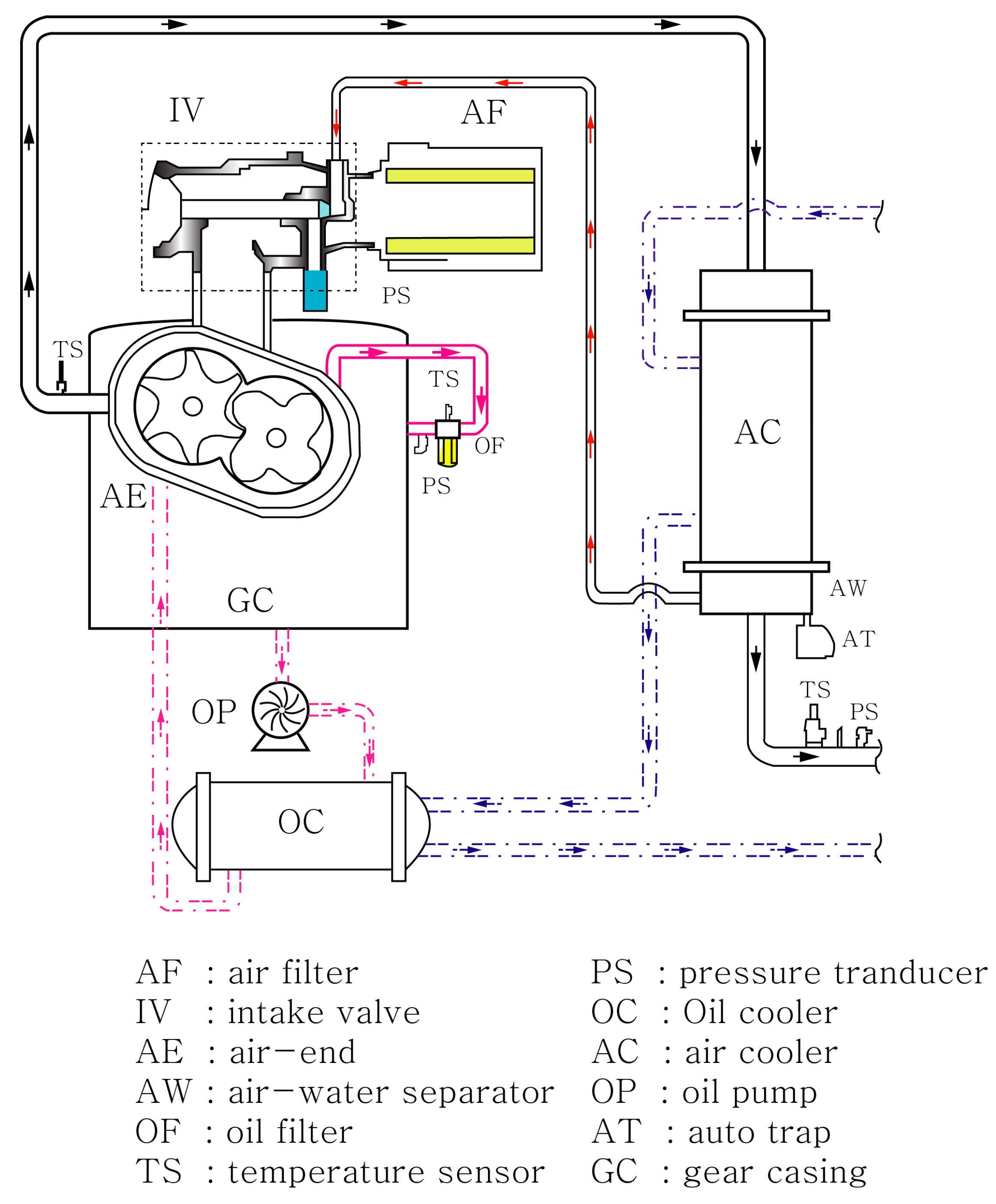
The experimental equipment used in this study was prepared to test the performance of the oil-free screw air-end. It was fabricated based on the flowchart shown in Figure 8, and is based on the quality standard specified in the volumetric compressor test and inspection method [17]. The atmospheric 25 °C working fluid, i.e., air, flows into the screw compressor through the air-water separator and the air filter. The air is compressed through the variation of the enclosed volume by the rotation of the female and male rotors. The experimental equipment is designed to record and store signals generated by instruments, such as temperature and pressure sensors, installed between each component part to a data acquisition system. The experimental model applied to this study has a cooling jacket, and the temperature of the inlet and the outlet of the cooling oil are maintained at 25 ± 3 °C. Experiments were carried out in the range of the ambient temperature and the inlet air temperature not exceeding 20 ± 1 °C. 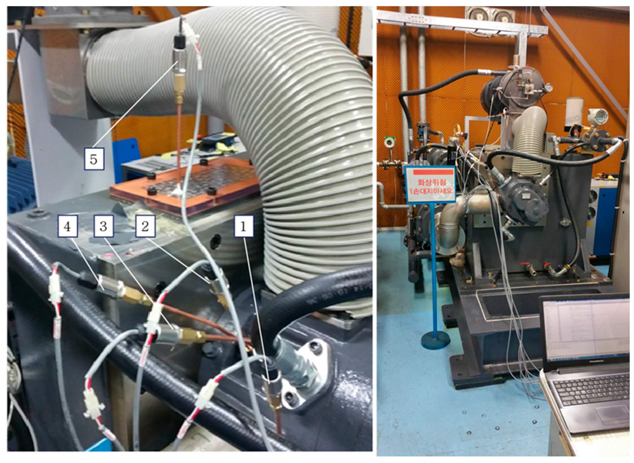Figure 9 shows the experimental apparatus consisting of a system based on the schematic diagram of Figure 8, as previously mentioned.

It is difficult to measure the pressure of the inflow air into the screw compressor according to the compression process. This is because the compression progresses as the enclosed volume formed by the compressor housing and the inner rotor continuously changes. In addition, the rotation speed of the male rotor is 13,000 rpm, and the rotation speed of the male rotor tip is 152.47 m/s. One rotation per 4.6 ms requires a data storage device with a high sampling speed, and a pressure sensor with a high resonance frequency.

The data processor uses a 100 kHz DAQ mode for each pressure sensor. The pressure transducer adopts a model to satisfy the condition of 0.3% precision, 1 ms response time, and operating pressure range of −0.1~0.3 MPa. The left figure in Figure 9 shows the pressure transducer inserted at five positions corresponding to the rotation angle (6~290°) of the male rotor, in order to measure the periodic pressure signal from the start of compression to the discharge part. In order to represent the measured pressure signal in the form of a pressure curve for the rotor, pressure curves are derived through signal combinations at each position.

5. Results and Discussion

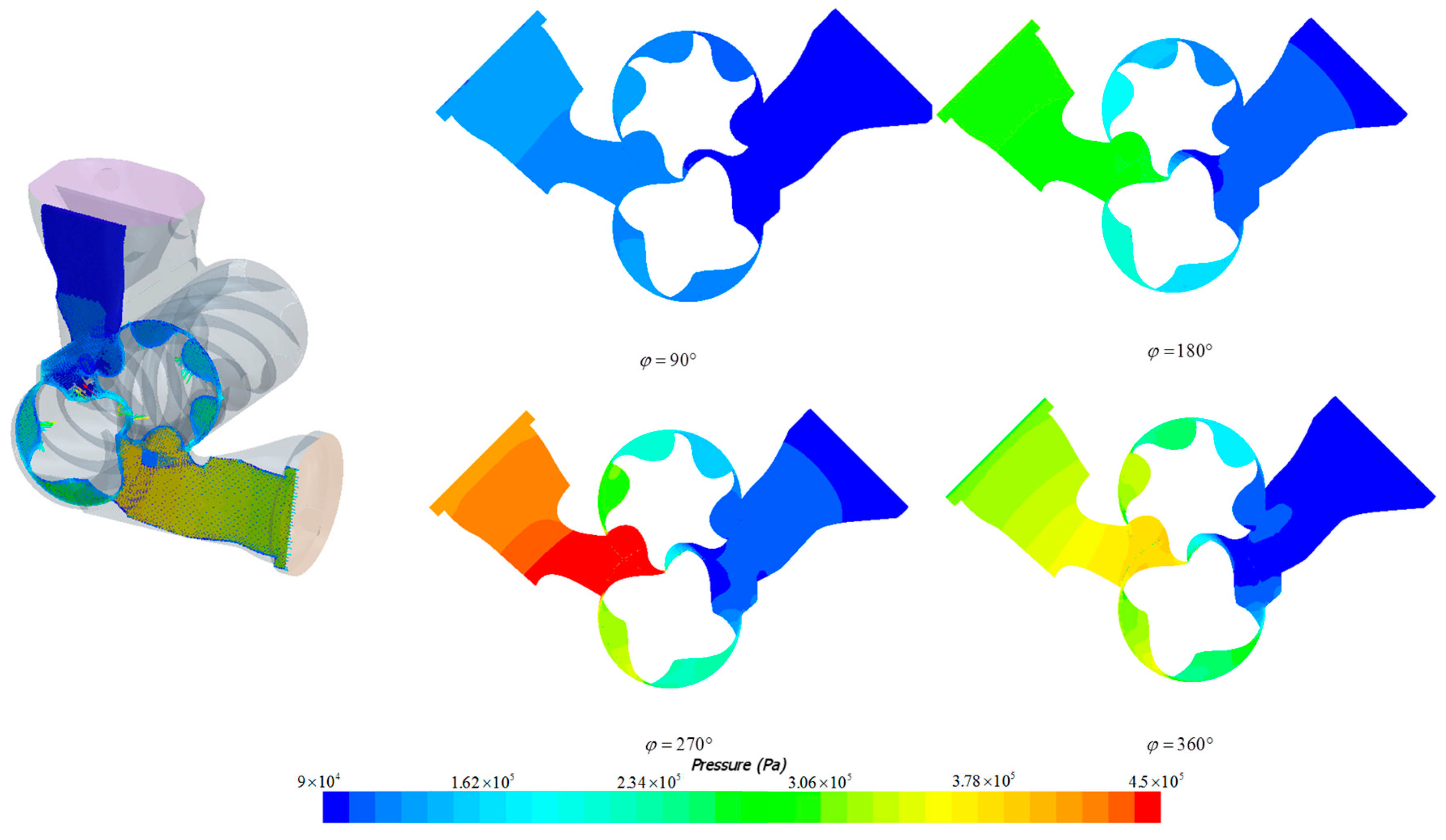
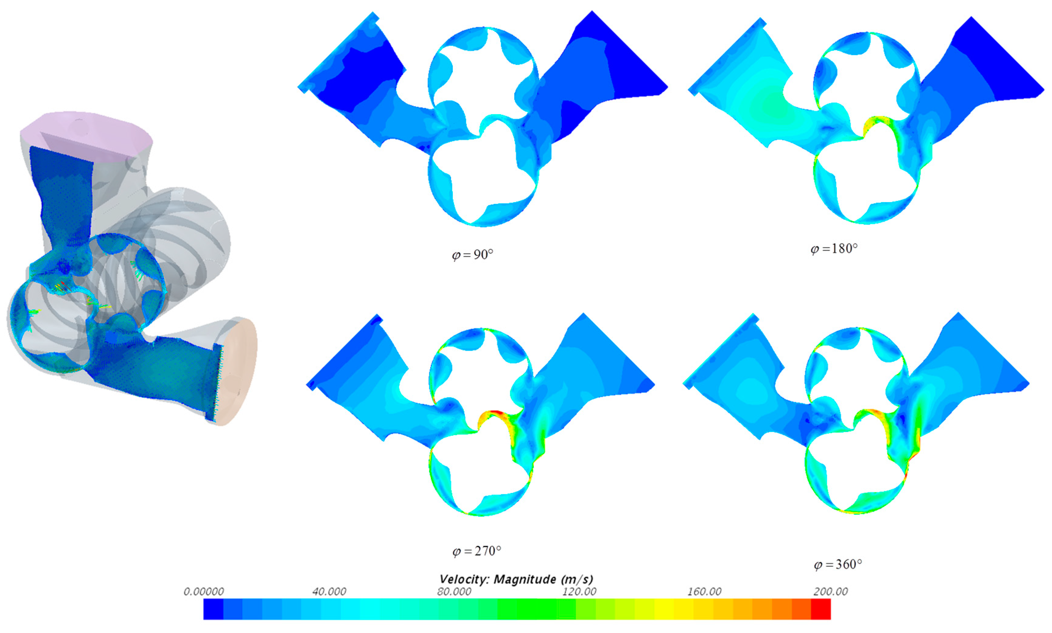
Figure 10 and Figure 11 show the pressure and velocity distributions at the cross-section of 15 mm from the end of the screw compressor housing.

The male rotor rotation angle shows a pressure distribution change by 90° at the 90~360° angle range in the converted time step. As can be seen from the results, as the rotor rotation angle increases, the suction port shows a value of about 100 kPa lower than the atmospheric pressure, and suction of the operating air is induced.

The compression stroke finishes from the female and male rotor of the discharge port, and the pressure gradually decreases from the end of the rotor lobe toward the discharge port. Figure 10 shows that the maximum value of the pressure at the end of the lobe is about 370 kPa, and the pressure at the outlet port is 317 kPa. The volume gradually increases as the enclosed volume decreases between the rotors.

As the rotor rotation angle increases, the velocity of the fluid out of the rotor is about 26 m/s. As the rotor moves toward the discharge port, the velocity decreases at about 40 m/s at the neck-narrowing portion. The velocity decreases at the end of the discharge port, and the value of about 10 m/s is calculated.

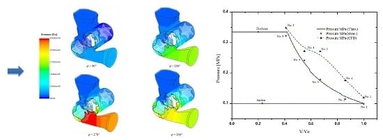
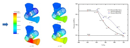
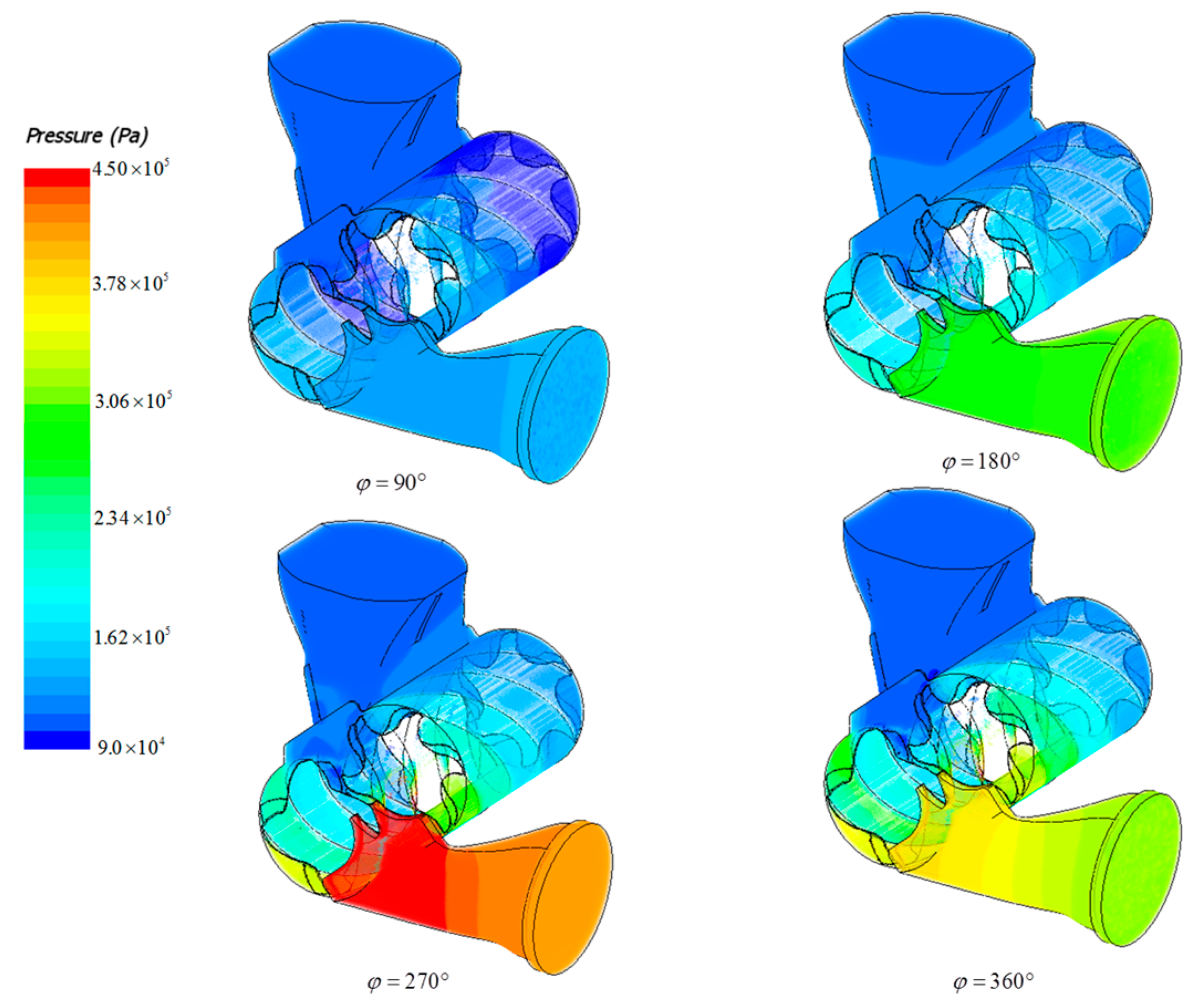
Figure 12 shows the volume rendering results of the pressure distribution according to the rotation angle change. The discharge port reduces the friction caused by the kinetic energy, and at the same time the ability to reduce the dynamic energy with the working fluid to the static pressure. Therefore, when the pressure of the working fluid is completed, the compression stroke between the ends of the rotor due to the shape of the discharge port is 270°. The pressure of the working fluid in which the compression stroke has completed is about 420 kPa. 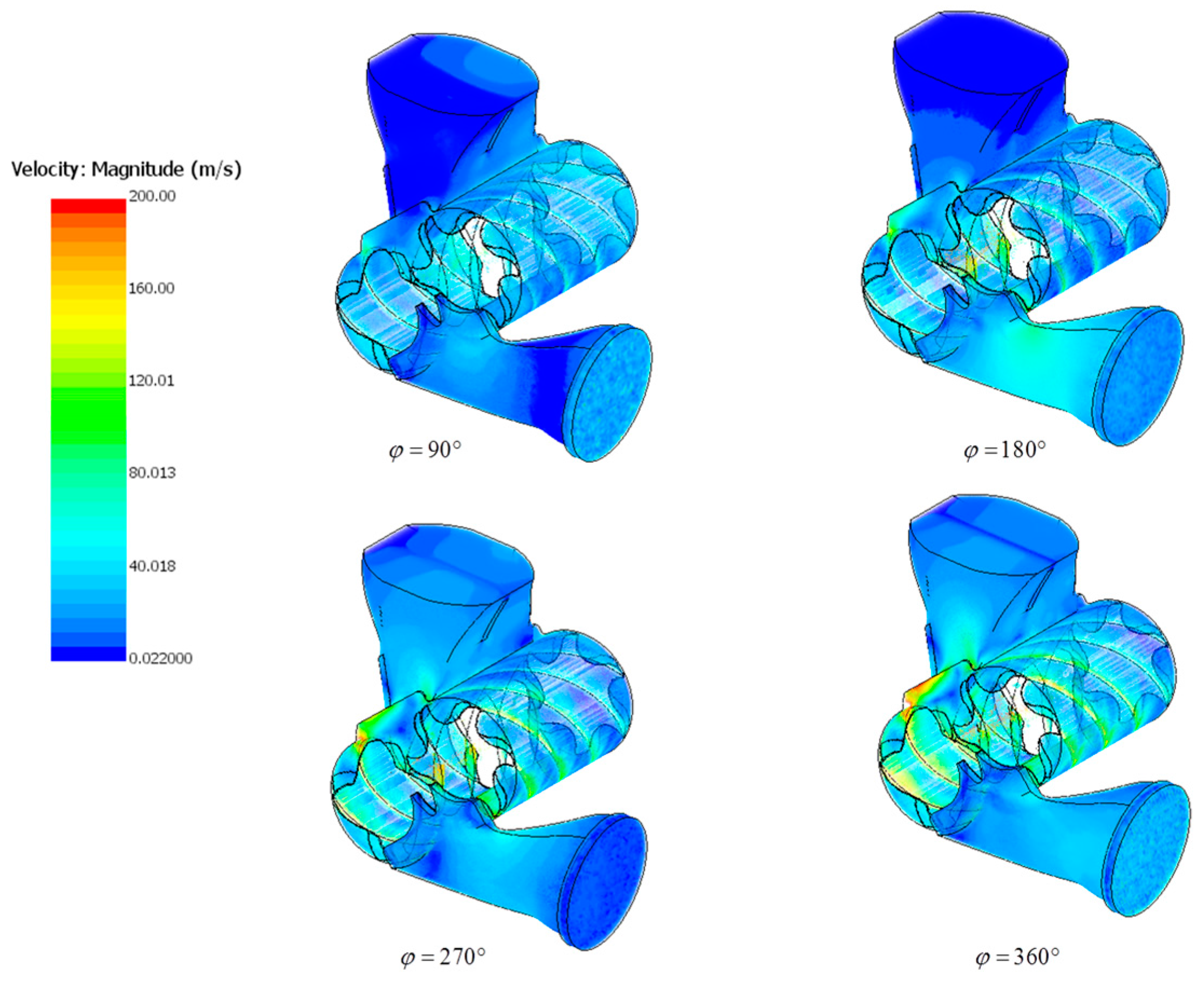Figure 13 shows the rendering calculation results of the velocity distribution volume according to the rotation angle change.

This shows that the kinetic energy increases locally at the velocity of 200 m/s in the suction port direction at the end surface of the discharge port in the direction of the discharge port, with an average of about 140 to 160 m/s along the seal line of the screw rotor.

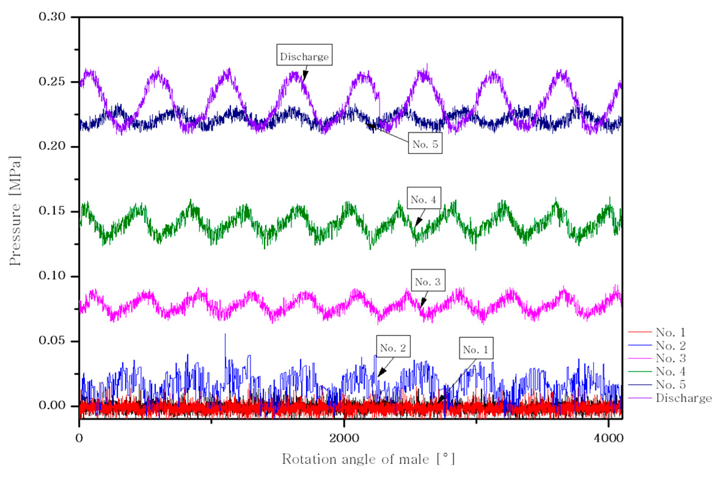
Figure 14 shows a periodical pressure change signal measured over the entire process in the compression stroke. As shown in Figure 13, the measurement values are shown at each of the positions 1~5 as described above, in order to measure the periodic pressure signal from the start of compression to the discharge part, according to the rotation angle of the rotor. The signal measured through this experiment is defined as a function of the pressure curve for the male rotor. By using this value, we set the polynomial function form to the outlet boundary condition of the CFD analysis.

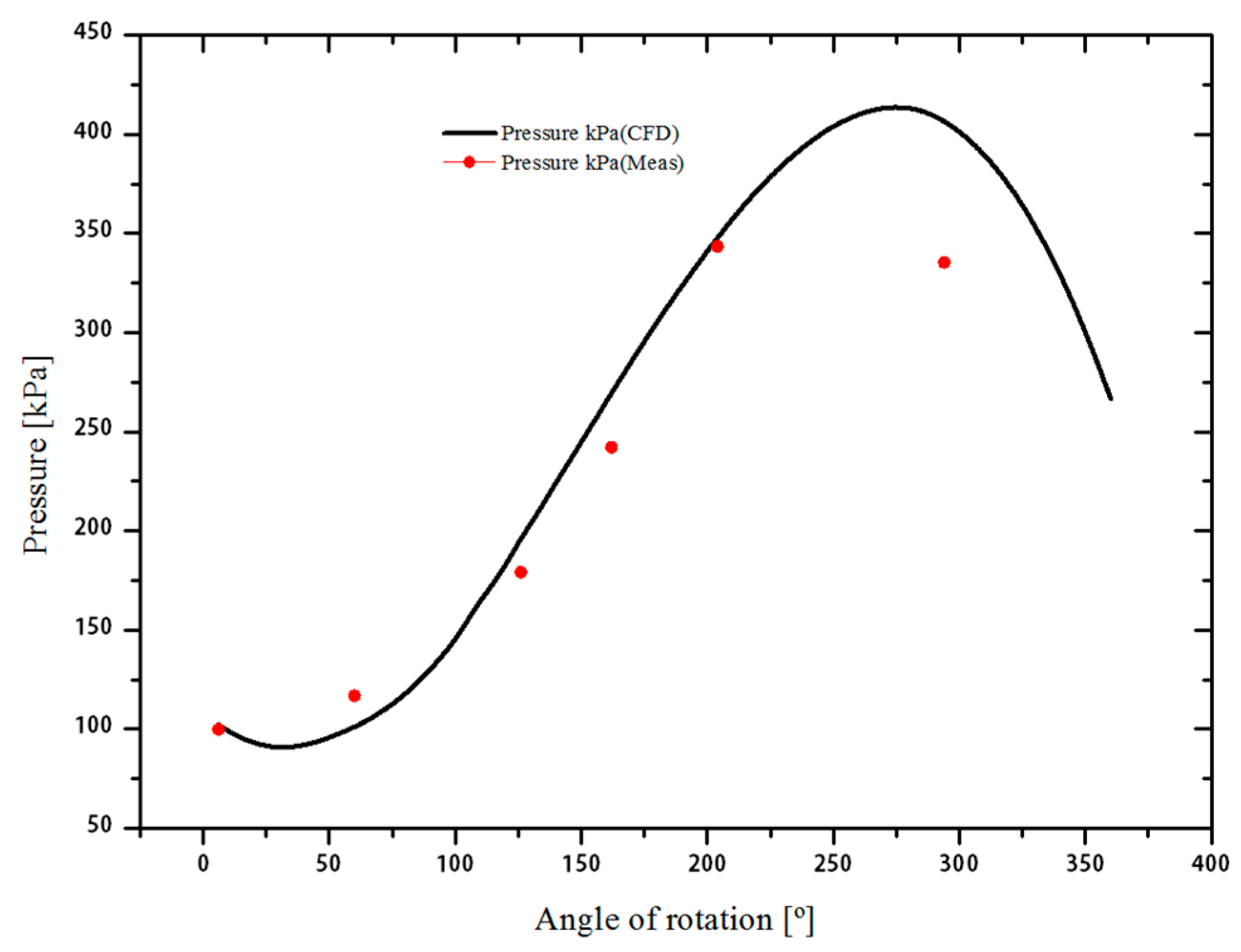
Figure 15 compares the change in pressure at the outlet with changes in rotation angle of the male rotor. The measured sample data are the mean values of the pressure measured at the place where the five pressure transducers are installed, and the exit pressure boundary condition is set as the interpolation value for the pressure value at each position, because the number of sample data is small. Therefore, it is confirmed that the error rate with respect to the pressure value increases after 200° of rotation angle.

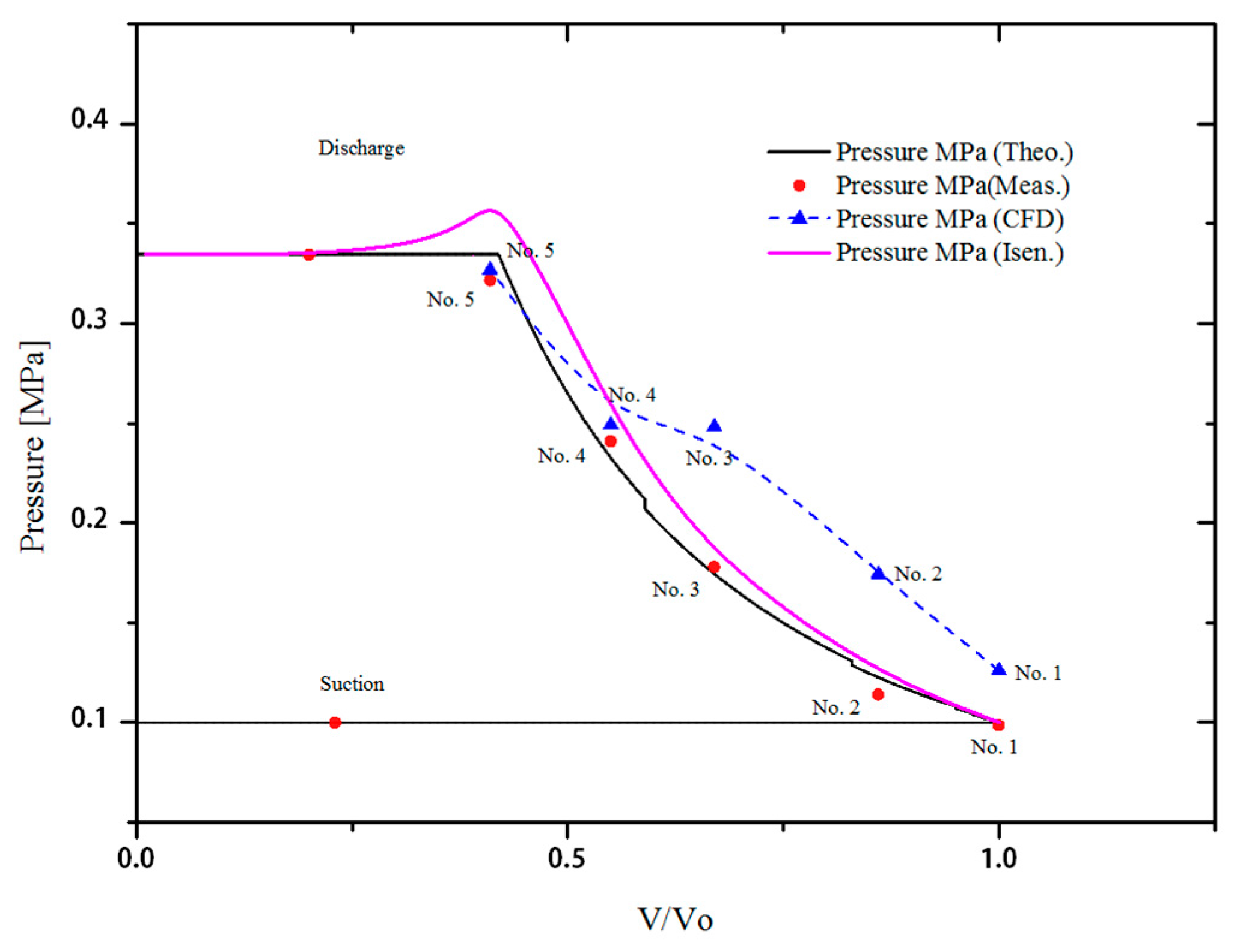
Figure 16 compares the theoretical and experimental measurements and CFD for the p-V indicator diagram. The experimental model of this study showed that the cooling jacket that was installed cooled the working fluid during the compression process, resulting in a measured value that was close to the isothermal process. It is confirmed that the CFD results are similar to the curve of the isentropic process, because heat exchange is not performed in the adiabatic condition.

6. Conclusions

In this study, we developed a MATLAB-based rotor profile program to generate the gear shape, which is an important factor that affects compressor performance. Based on this, the reliability was verified by CFD analysis using the finite volume method, and comparison of the experimental results. Through the experiment of the screw compressor, we have obtained sample data to be applied to the basic boundary conditions of the CFD analysis, and confirmed that the error rate with respect to the pressure value increases after 200° rotation of the rotor according to physical time. The results of the comparison of the theoretical and measured values of the p-V diagram of the experimental model are derived, and it is confirmed that the measured value is very similar to the theoretical calculation value. However, the p-V diagram calculated through the CFD analysis has a deviation from the theoretical and measured values. This is because the wall surface condition inside the housing is set as the adiabatic condition, and heat exchange by the cooling jacket is not performed, so that it is similar to the curve of the isentropic process. Also, additional work shall be performed to investigate the influence of the meshing parameters as well as time-step in order to improve the convergence of the solution.

References

1. Stosic, N.; Hanjalic, K. General Method for Screw Compressor Profile Generation. In Proceedings of the 1996 International Compressor Engineering Conference at Purdue, West Lafayette, IN, USA, 23–26 July 1996; pp. 157–162. [Google Scholar]
2. Tang, Y.; Fleming, J.S. Obtaining the Optimum Geometrical Parameters of a Refrigeration Helical Screw Compressor. In Proceedings of the 1992 International Compressor Engineering Conference at Purdue, West Lafayette, IN, USA, 14–17 July 1992. [Google Scholar]
3. Stosic, N. On gearing of helical screw compressor rotors. Proc. Inst. Mechan. Eng. Part C J. Mech. Eng. Sci. 1998, 212, 587–594. [Google Scholar] [CrossRef]
4. Stosic, N.; Smith, I.K.; Kovacevic, A. Optimisation of screw compressors. Appl. Therm. Eng. 2003, 23, 1177–1195. [Google Scholar] [CrossRef]
5. Stosic, N.; Smith, I.K.; Kovacevic, A.; Aldis, C.A. The Design of a Twin-screw Compressor Based on a New Rotor Profile. J. Eng. Des. 1997, 8, 389–399. [Google Scholar] [CrossRef]
6. Kovacevic, A. Boundary adaptation in grid generation for CFD analysis of screw compressors. Int. J. Numer. Methods Eng. 2005, 64, 401–426. [Google Scholar] [CrossRef]
7. Voorde Vande, J.; Vierendeels, J.; Dick, E. Development of a Laplacian-based mesh generator for ALE calculations in rotary volumetric pumps and compressors. Comput. Methods Appl. Mech. Eng. 2004, 193, 4401–4415. [Google Scholar] [CrossRef]
8. Rane, S.; Kovacevic, A. Advances in Engineering Software Algebraic generation of single domain computational grid for twin screw machines. Part I. Implementation. Adv. Eng. Softw. 2017, 107, 38–50. [Google Scholar] [CrossRef]
9. Rane, S.; Kovacevic, A.; Kethidi, M. CFD Modelling in Screw Compressors with Complex Multi Rotor Configurations. In Proceedings of the 2012 International Compressor Engineering Conference at Purdue, West Lafayette, IN, USA, 16–19 July 2012. [Google Scholar]
10. Steger, J.L.; Benek, J.A. On the use of composite grid schemes in computational aerodynamics. Comput. Methods Appl. Mech. Eng. 1987, 64, 301–320. [Google Scholar] [CrossRef]
11. Li, Y.; Paik, K.J.; Xing, T.; Carrica, P.M. Dynamic overset CFD simulations of wind turbine aerodynamics. Renew. Energy 2012, 37, 285–298. [Google Scholar] [CrossRef]
12. Suman, A.; Ziviani, D.; Gabrielloni, J.; Pinelli, M.; De Paepe, M.; Van Den Broek, M. Different Numerical Approaches for the Analysis of a Single Screw Expander. Energy Procedia 2016, 101, 750–757. [Google Scholar] [CrossRef]
13. Choi, S.H.; Kim, D.H. A study on performance analysis of screw rotor profile. J. Korean Soc. Precis. Eng. 1996, 13, 69–76. [Google Scholar]
14. Park, D.K.; Lee, K.S. Performance analysis of screw air compressor. Proc. Korean Soc. Mech. Eng. 2000, 26, 184–193. [Google Scholar] [CrossRef]
15. Korea Institute of Science and Technology. A Study on the Development of an Optimum Design Technique of Screw Rotors; Internal Report; Ministry of Science and Technology: Gwacheon, Korea, 1990. (In Korean)
16. Hadzic, H. Development and Application of a Finite Volume Method for the Computation of Flows around Moving Bodies on Unstructured, Overlapping Grids. Ph.D. Thesis, Hamburg University of Technology, Hamburg, Germany, 2005. [Google Scholar]
17. Korean Standards Association. Displacement Compressors-Testing Methods; KS B 6351; Korean Standards Association: Seoul, Korea, 2014. [Google Scholar]
18. Lee, J.Y. Effects of the Opening Angle of Suction/Discharge Ports on the Performance of 4 × 6 Oil-free Screw Compressor. Ph.D. Thesis, Sungkyunkwan University, Seoul, Korea, 2016. [Google Scholar]
Figure 1. The coordinate systems of the modeled screw rotors.
Energies 10 00945 g001
Figure 2. A detailed view of the rotor profile.
Energies 10 00945 g002
Figure 3. MATLAB-based screw rotor profile design program.
Energies 10 00945 g003
Figure 4. A detailed view of the overlap region with some definitions and notations [16].
Energies 10 00945 g004
Figure 5. Control volume of the twin-screw compressor.
Energies 10 00945 g005
Figure 6. The grid section created by the hole cutting process in this study.
Energies 10 00945 g006
Figure 7. The grid dependency test.
Energies 10 00945 g007
Figure 8. Schematic diagram of the test bench.
Energies 10 00945 g008
Figure 9. Experimental setup of the test bench [18].
Energies 10 00945 g009
Figure 10. Cross-section of the pressure distribution in the vicinity of the discharge port.
Energies 10 00945 g010
Figure 11. Cross-section of the velocity distribution in the vicinity of the discharge port.
Energies 10 00945 g011
Figure 12. Volume rendering of the pressure distribution according to the angle of rotation.
Energies 10 00945 g012
Figure 13. Volume rendering of the velocity distribution according to the angle of rotation.
Energies 10 00945 g013
Figure 14. The periodical pressure signals versus male rotor rotation angle.
Energies 10 00945 g014
Figure 15. Comparison results of pressure distribution at the discharge port between CFD and measurement.
Energies 10 00945 g015
Figure 16. Comparison results of pressure distribution between the theoretical values, CFD and measurements on the p-V indicator diagram.
Energies 10 00945 g016