1. Introduction
The day-ahead electricity market (EM) is a crucial component in the EM system [
1]. In recent years, wind power resources have experienced an unprecedented growth in the day-ahead EMs worldwide. Studies on wind power bidding in the day-ahead EM with wind power penetration are too numerous to enumerate one by one. References [
2,
3,
4] etc., for reasons such as low marginal cost of wind power producer (WPP) etc., hold that the bidding mode (BM) of a WPP is to only send the independent system operator (ISO) its power output plan for each period of the next day (namely, BM 1). The ISO ensures the wind power accommodation according to every WPP’s day-ahead power output plan, but a WPP should be financially punished when its real time power output deviates from the day-ahead bidding one [
3]. References [
5,
6,
7,
8,
9] etc., based on actual EMs such as PJM (Pennsylvania-New Jersey-Maryland) etc., point out that the BM of a WPP is to provide ISO a bidding curve for each period of the next day (namely, BM 2). A bidding curve consists of bidding price and power output. According to these day-ahead bidding curves provided by WPPs, ISO, within a certain range of forecasted power outputs corresponding to each WPP, can dispatch the power outputs of WPPs in the day-ahead EM. However, a WPP should also be financially punished when its real time power output deviates from the day-ahead scheduled one [
9]. In this work, we believed that different BMs adopted by WPPs may lead to different market results such as profits, clearing prices and operation cost of the power system. Hence, one motivation of this work is to experimentally compare those two BMs adopted by WPPs in day-ahead EM.
In addition, owning to the inherent intermittence, fluctuation, and low predictability of wind power output, uncertainties grow significantly with the increasing penetration of wind power resources, which pose major challenges to wind power accommodation in the EM [
10]. Therefore, many references propose that the wind power accommodation can be improved by modifying the market clearing model (MCM) corresponding to ISO in day-ahead EM. References [
9,
11,
12,
13] applied the stochastic optimization (SO) method in the market clearing procedure. The SO-MCM significantly increases the number of constraints in MCM by generating real time wind power output stochastic scenarios (WPOSSs) based on real time wind power output probability distributions. The market clearing results (scheduled power results and clearing price of every node) can be obtained by optimizing the expected value of the objective function in SO-MCM [
9]. This approach takes into account different security constraints of power system under different WPOSSs, and improves, to a certain extent, the wind power accommodation capacity of power system. However, SO-MCM still has the following shortcomings, thereby greatly reducing the feasibility and rationality of this method [
14,
15]: (1) in practice, the probability distribution of real time wind power output is difficult to obtain; (2) a small number of real time WPOSSs may lead to a reduction of the ability of the power system to resist random real time wind power output deviations from its day-ahead (bidding or scheduled) one; (3) a large number of WPOSSs may significantly increase the computational complexity of the model, thereby resulting in solving difficulties. In order to overcome these abovementioned shortcomings, recently, robust optimization (RO) methods are applied to the construction of power system dispatch models by many studies. Reference [
16] proposed a two-stage robust security constraint unit-commitment (SCUC) model. The key idea of this two-stage robust SCUC model is to determine the optimal unit-commitment (UC) solution in the first stage which leads to the least operation cost for the worst wind power output scenario (WPOS) in the second stage. However, this approach is very conservative due to the optimization for the operation cost of the worst WPOS in the second stage. In Reference [
17] the authors combined the stochastic and robust approaches using a weight factor in the objective function to address the conservativeness issue. Reference [
18] employed the Affine Policy (AP) to formulate and solve the robust security constraint economic dispatch (SCED) model. Reference [
19] proposed a robust optimization framework for robust SCUC and robust SCED which repeatedly calculates the UC and ED solutions in the first stage to optimize the operation cost of the basic WPOS but to pass the security test in the second stage. RO-based power system dispatch models do not need the probability distribution of real time wind power output. The number of constraints need not be significantly increased with the increase of the size of uncertainty set [
19]. The optimal robust UC and ED solutions can satisfy every unit-wise and system-wise constraint under the worst WPOS [
19], which means RO-based power system dispatch models can not only improve wind power accommodation but also maintain low computational complexity so as to promote the application of these models in practice. However, the approaches in [
16,
17,
18,
19] cannot be introduced directly for modification of MCM in day-ahead EM because it is not mentioned in those studies how to price the power outputs, loads, reserves and deviations (uncertainties). Recently, in study of Ye et al. [
20], this shortcoming is made up by combining cost causation principle and locational marginal price (LMP) in robust SCUC and robust SCED modeling approaches so as to successfully modify the MCM in day-ahead EM by using a RO method. Therefore, inspired by [
20], in this work, no matter which BM WPPs adopt in day-ahead EM bidding, the MCM corresponding to ISO will be modified by using a RO-method in order to make the power system accommodate any deviation caused by real time wind power uncertainties within a certain range.
Finally, a WPP participating in EM bidding aims at profit maximization. In a day-ahead EM, there are many participants competing with each other. In addition to real time wind power uncertainties, WPPs, like other conventional generation companies (GenCOs), are faced with complex market environment conditions, such as imperfect and incomplete information. Hence, there are many similarities between EM modeling approaches with and without WPPs participating in market bidding. EM modeling approaches proposed in [
21,
22,
23,
24,
25] are based on game theory. EM modeling approaches proposed in [
26,
27,
28,
29,
30,
31] are based on machine learning algorithms. Recently, many relevant studies take renewable energy (i.e., wind power) bidding into account. Reference [
32] supposed that a WPP strategically bids with BM 2 in day-ahead EM, and put forward a closed-form analysis on WPP’s strategic behavior based on the Stackelberg game model. Reference [
33] proposed an autoregressive integrated moving average (ARIMA) model to obtain the optimal bidding strategy for a WPP who bids with BM 2 in day-ahead EM. The authors of [
34] studied the behaviors of strategic WPPs bidding in EM with BM 1 based on Cournot game model. In Reference [
35] an imbalance cost minimization bidding strategy for a BM 1 adopted WPP through forecasting the real time wind power probability distribution functions was proposed. Reference [
36] analyzed the strategic behavior of a BM 1 adopted WPP in day-ahead EM based on Roth-Erev reinforcement learning algorithm. In [
37], a stochastic programming problem was proposed for obtaining the optimal offering and operating strategy for a large wind-storage system adopting BM 2. Reference [
38] considered the uncertainty on electricity price through a set of exogenous scenarios and solved the bidding problem of a BM 1 adopted thermal-wind power producer by using a stochastic mixed-integer linear programming approach. The authors in reference [
39] proposed a two-stage stochastic bidding model based on kernel density estimation (KDE) for a BM 2 adopted WPP to obtain the optimal day-ahead bidding strategy. The approaches in [
24,
25,
33,
35,
37,
38,
39] resulted in repeatedly solving multi-level mathematical programming models for every participant, the computational complexities of which limit their applications in more realistic situations. The methods proposed in [
21,
22,
23,
32,
34] produced sets of nonlinear equations which are difficult to solve or have no solutions. The approaches in [
26,
27,
28,
29,
30,
31,
36] belong to the agent-based EM modeling approaches, in which every bidding participant is considered as an agent who has the ability of adaptive learning so as to improve its profit during process of repeated bidding in market. Table-based reinforcement learning (TBRL) algorithms are usually proposed in depicting agents’ adaptive learning approaches in EM bidding, such as the Q-learning-based approach proposed in [
26,
27], simulated annealing Q-learning-based approach proposed in [
28], Roth-Erev reinforcement learning-based EM test bed (called Multi-Agent Simulator of Competitive Electricity Markets or MASCEM) proposed in [
29,
36], SARSA (state-action-reward-state-action)-based approach proposed in [
30], fuzzy Q-learning-based approach proposed in [
31], etc. By using agent-based EM modeling approaches, it is neither necessary to repeatedly solve multi-level mathematical programming models for every agent, nor to establish sets of nonlinear equations which are difficult to solve or have no solutions. Low computational complexity and low reliance on common knowledge make these approaches more applicable in EM modeling [
26]. However, in TBRL algorithms, both an agent’s action (i.e., bidding strategy) and state (i.e., market environment) sets must be assumed as discrete, otherwise it will cause the problem of “curse of dimensionality”, which does not conform to the actual situation of the day-ahead EM and hinders a strategic WPP to obtain its globally optimal bidding strategies no matter which BM it adopts. So far as we know, there is no reasonable way to solve this issue in the published literature studying wind power and other renewable energy bidding in EMs. Recently, Chen [
40] proposed a modified reinforcement learning (RL) algorithm called Least Squares Continuous Actor-Critic (LSCAC) algorithm which can make both the action and state sets continuous without causing the problem of “curse of dimensionality”. Therefore, another motivation of this work was to apply for the first time the LSCAC algorithm for modeling the strategic bidding behaviors of WPPs in day-ahead EMs. On the one hand, this approach properly solved the contradiction of making every agent’s action and state sets continuous and causing the “curse of dimensionality” problem. On the other hand, it can provide a reasonable EM test bed to simulate and experimentally compare those two BMs adopted by WPPs in a day-ahead EM.
Therefore, the main novelty of this paper can be summarized as to firstly propose the LSCAC-based day-ahead EM modeling approach for strategic WPPs under robust market clearing conditions. The purpose for employing robust MCM is to improve wind power accommodation by reconstructing the market clearing mechanism. The motivation of proposing the LSCAC-based EM modeling approach is to assist strategic WPPs to make more appropriate bidding decisions so as to improve both the WPPs’ profits and the economic efficiency of the whole market compared with TBRL-based approaches. Moreover, comparison between different BMs can offer some suggestions about improving wind power resources development and market economic efficiency.
The rest of this paper is organized as follows: in
Section 2, the concrete mathematic formulations of WPPs’ different BMs and the robust day-head MCM are proposed.
Section 3 puts forward the proposed LSCAC-based day-ahead EM modeling approach for WPPs.
Section 4 conducts the simulations and comparisons.
Section 5 concludes the paper.
4. Simulations and Discussions
4.1. System Data
In this section, by implementing the robust MCM mentioned in
Section 2, our proposed day-ahead EM modeling approaches under different BMs are simulated on the IEEE 30-bus test system with five strategic WPPs [
9]. Matlab R2014a is utilized to conduct our simulations.
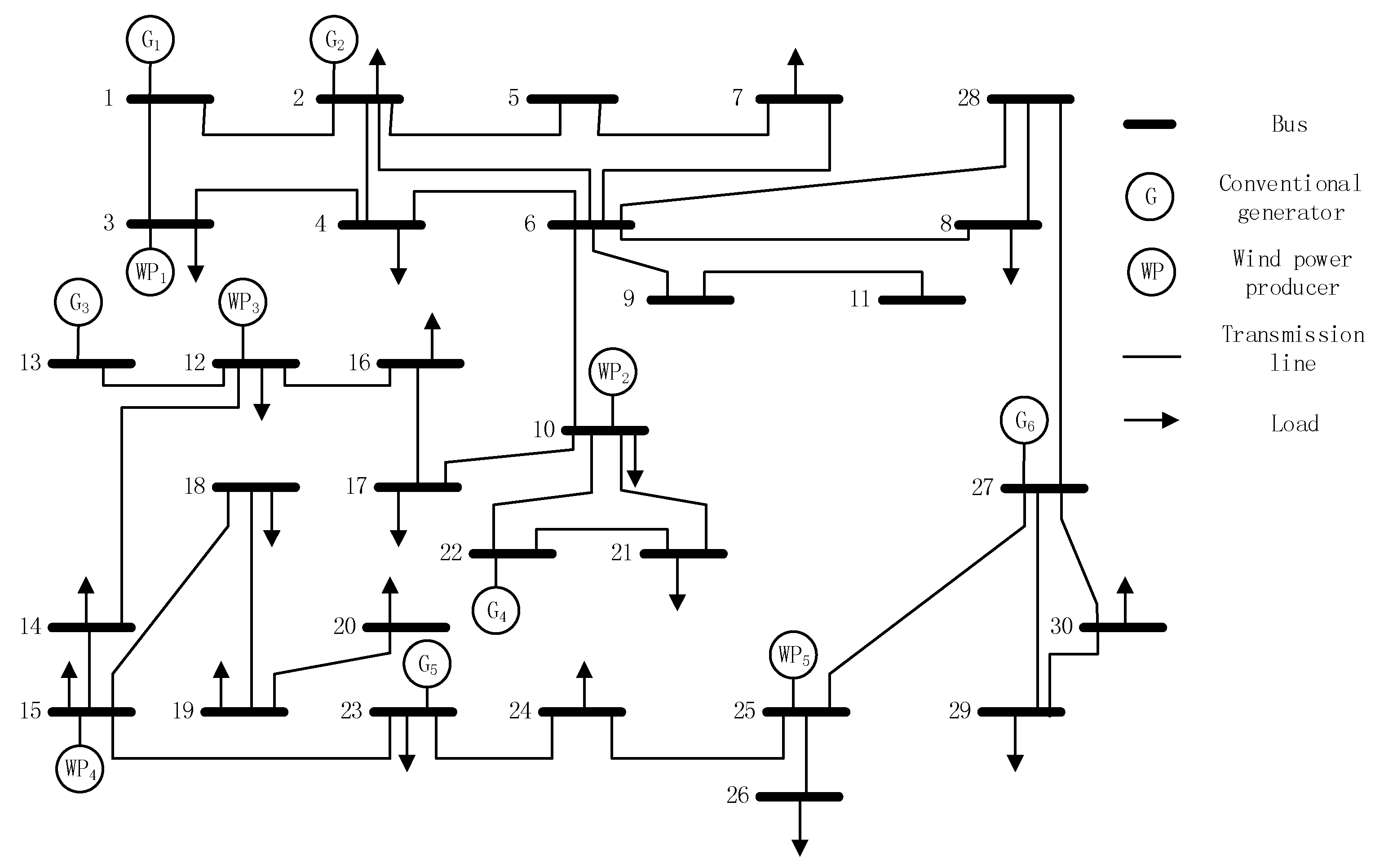
Figure 1 shows the schematic structure of the test system.
Table 1 depicts the predicted single period loads distributed in different buses [
42]. Consistent with the assumptions in
Section 2, any uncertainties in this test system are not caused by loads. Parameters of conventional generators can be seen in
Table 2, and the predicted power output intervals of the five WPPs which are the crucial components of the uncertainty set, are listed in
Table 3. For the sake of simplicity and without losing generality, we assume the power output interval of WPP
i(
) predicted by ISO is the same as that predicted by WPP
i(
) itself.
4.2. Robust MCM Testing
The value of budget parameter
is related to the size of the uncertainty set. The smaller
is, the smaller is the size of uncertainty set estimated by ISO. That is to say the day-ahead market clearing procedure of ISO tends to be more deterministic with the decrease of the value of
(
). When
, it means the predicted power output of every WPP is deemed by ISO as a definite value which, according to Equation (1) and [
10,
19,
20], is equal to the intermediate value of its power output interval, and the day-ahead MCM of ISO is completely turned into a conventional deterministic MCM similar to [
30]. However, uncertainties exist objectively in a power system with WPPs. If the market clearing procedure were implemented by ISO without considering enough uncertainties, the reserve capacity of the system dispatched in day-ahead might find it hard to accommodate deviations caused by WPPs’ power output uncertainties in real time, which can seriously affect the security of the system and cause huge extra costs such as wind-abandonment, etc. Therefore, market clearing results under different
values must be compared so as to verify the necessity of proposing robust MCM in day-ahead EM with wind power penetrations.
In this section, in order to facilitate the market clearing comparison, we assume every WPP is under BM 1 and sends the ISO the intermediate value of its power output interval. In fact, the same key conclusions obtained from market clearing comparisons can also be generated with other BM and strategies. Moreover, no matter what the ISO thinks the value of
is, the actual value of
which represents the objective existence of uncertainty is fixed, by us, to the number of WPPs in the system (
= 5).
Table 4 shows the market clearing results under different
values.
In
Table 4, because the marginal cost of every WPP is neglected [
3,
31], the “operation cost” in column 2 can be calculated by using
when the optimal ED solution is obtained. Moreover, the “uncertainty that cannot be accommodated” in column 3 means whether there exist uncertainty points in
that cannot be accommodated when the optimal ED solution is obtained. The “number of uncertainty poles that cannot be accommodated” in column 4 denotes the number of poles in
that cannot be accommodated when the optimal ED solution is obtained. From
Table 4, it can be concluded that:
The total operation cost increases with the increase of . However, uncertainties that cannot be accommodated tend to be eliminated by increasing . On one hand, it means the conservatism of ISO is improved with the increase of , which reduces the economic efficiency of scheduling to a certain extent. On the other hand, the operation cost is calculated based on the basic scenario (WPPs’ day-ahead bids), in which extra cost caused by uncertainties that cannot be accommodated is not taken into account. Although that extra cost is hard to be specifically calculated due to many reasons such as missing information about the real-time occurrence of uncertainty from day-ahead horizon etc., it can be considerable once any uncertainty that cannot be accommodated occurs in practice. Therefore, it is necessary to eliminate uncertainties that cannot be accommodated by reasonably increasing the value of .
When
, it means the ISO clears the market using the conventional deterministic MCM. The number of uncertainty poles that cannot be accommodated in case
is 22 which is significantly more than any other cases listed in
Table 4 (actually number of uncertainties that cannot be accommodated in case
is infinite). That is to say it is necessary to employ a modified MCM, such as our proposed robust MCM, in day-ahead EM with considerable uncertainties (i.e., WPPs).
Comparing cases of
and
, on one hand, there are no uncertainties that cannot be accommodated in both of the two cases; on the other hand, operation cost in case
is equal to that in case
. Moreover, increasing
means to increase the computational complexity of solving the robust MCM [
15,
16,
19,
20]. Hence, the proposed robust MCM with
is applied for market clearing in our subsequent simulations.
4.3. LSCAC-Based EM Modeling Approach Testing
In this section and our subsequent simulations, no matter under which BM, every WPP (agent) will start with experiencing a training process of 3000 iterations. During this training process, all WPPs consider the balance of exploration and exploitation when selecting bidding strategies (actions) in each iteration [
41]. After the training process, decision making process of 500 iterations will be implemented by every WPP, in which only greedy policy will be adopted when selecting actions in face of any state of the market. Moreover, we randomly set the action for every WPP at the beginning of the first training iteration because every WPP starts with limited experience in strategy selecting.
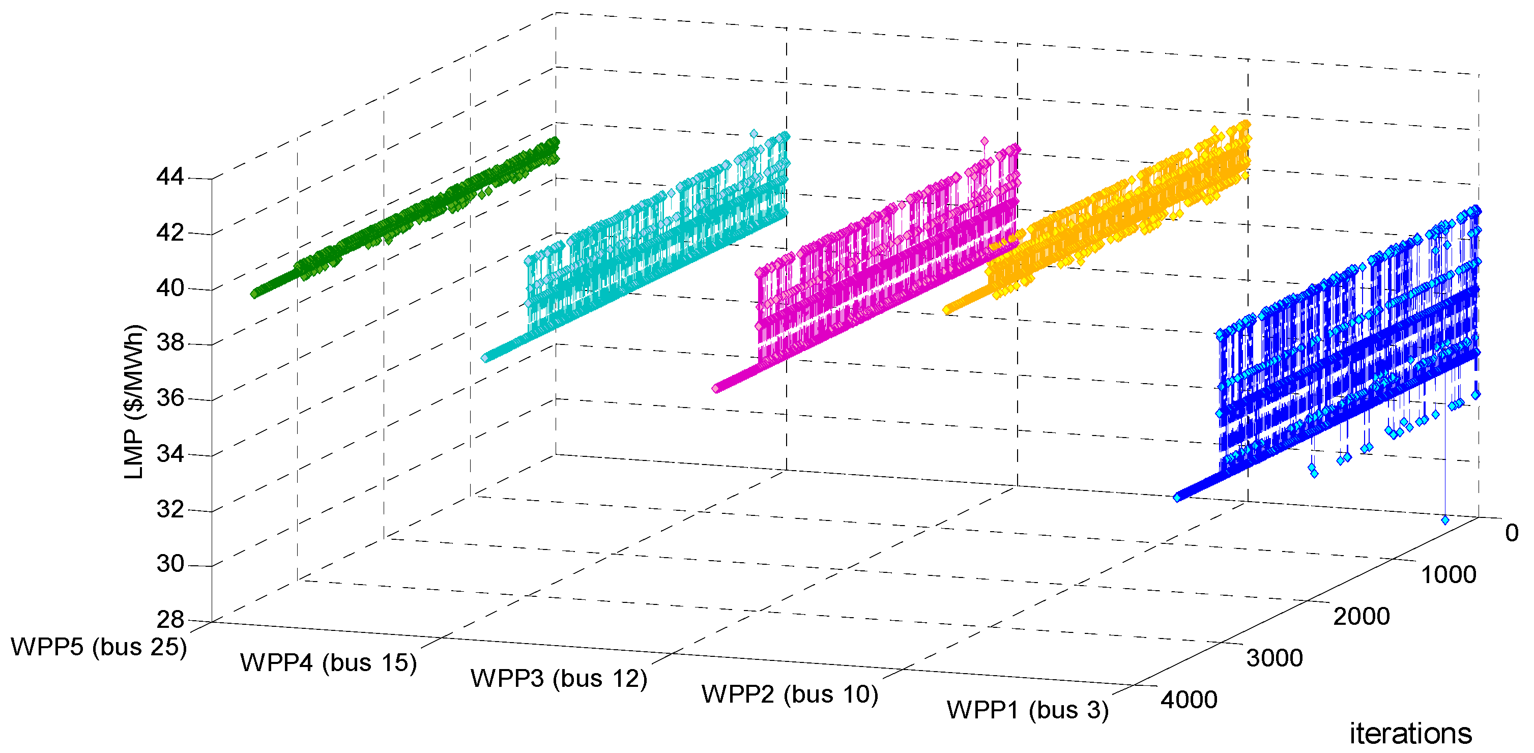
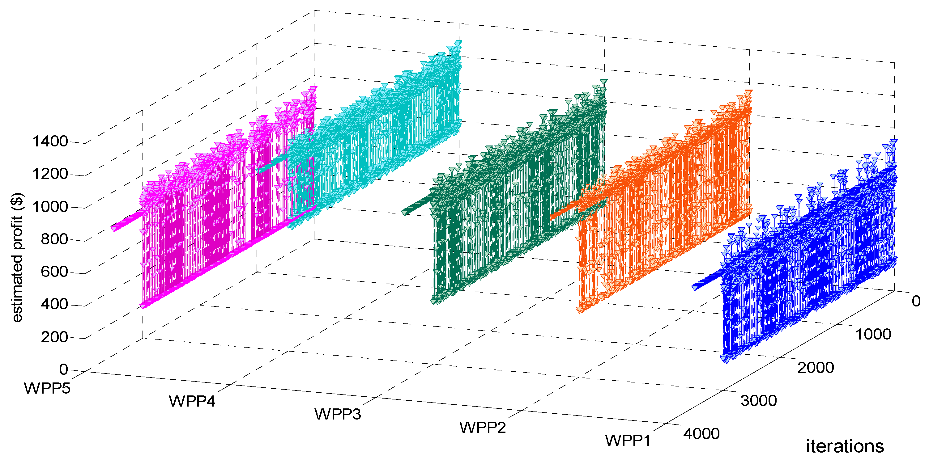
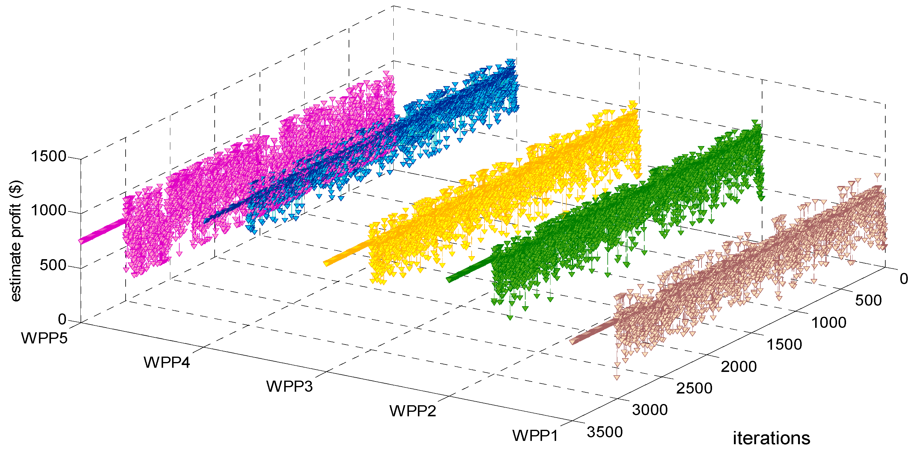
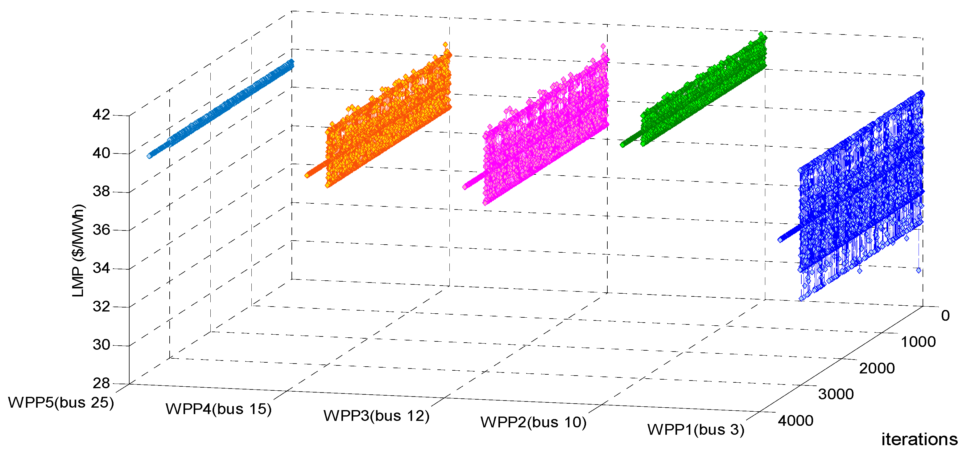
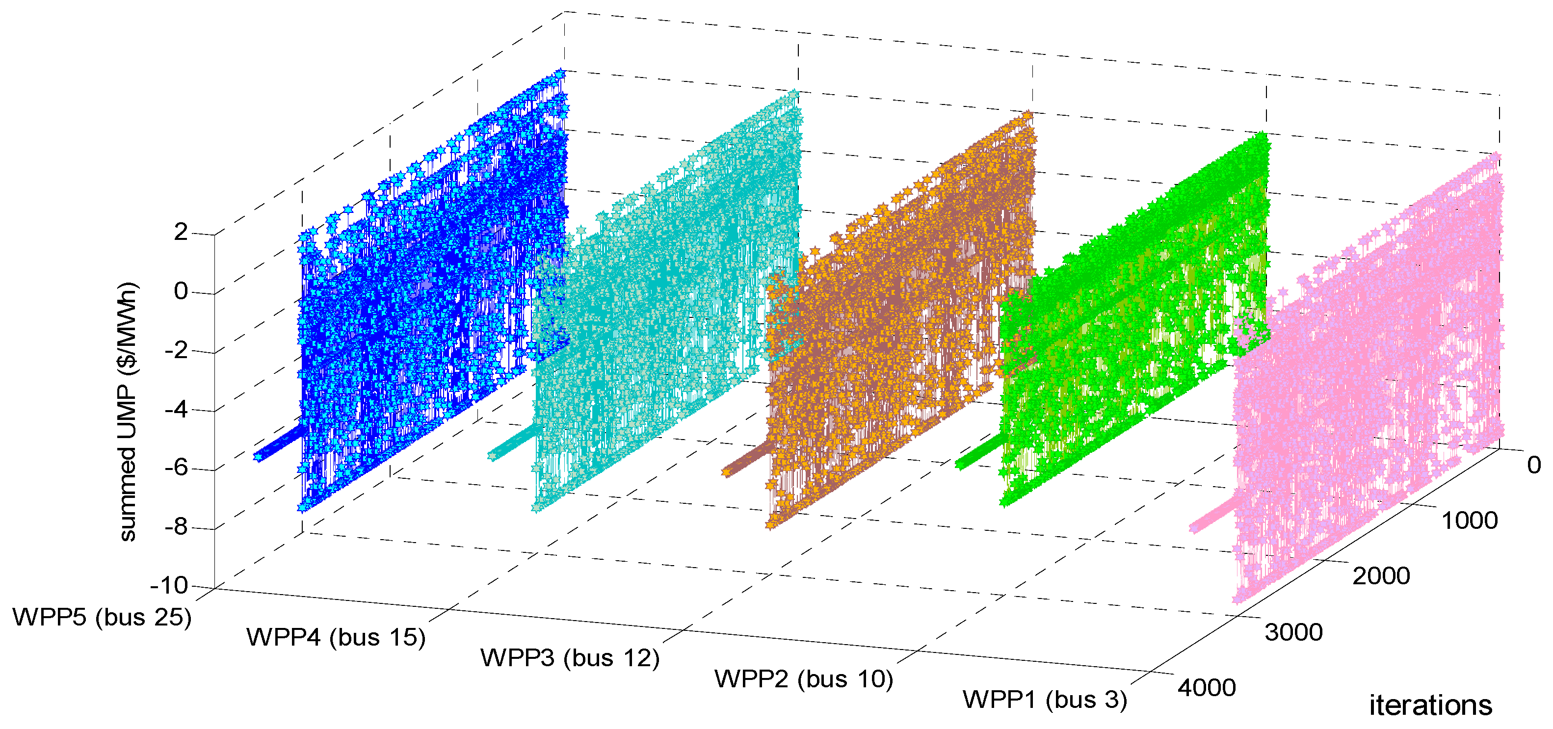
Testing and verifying whether our proposed LSCAC-based day-head EM approach under BM 1 reaches to dynamic stability or not after 3000 training iterations can be shown in
Figure 2,
Figure 3 and
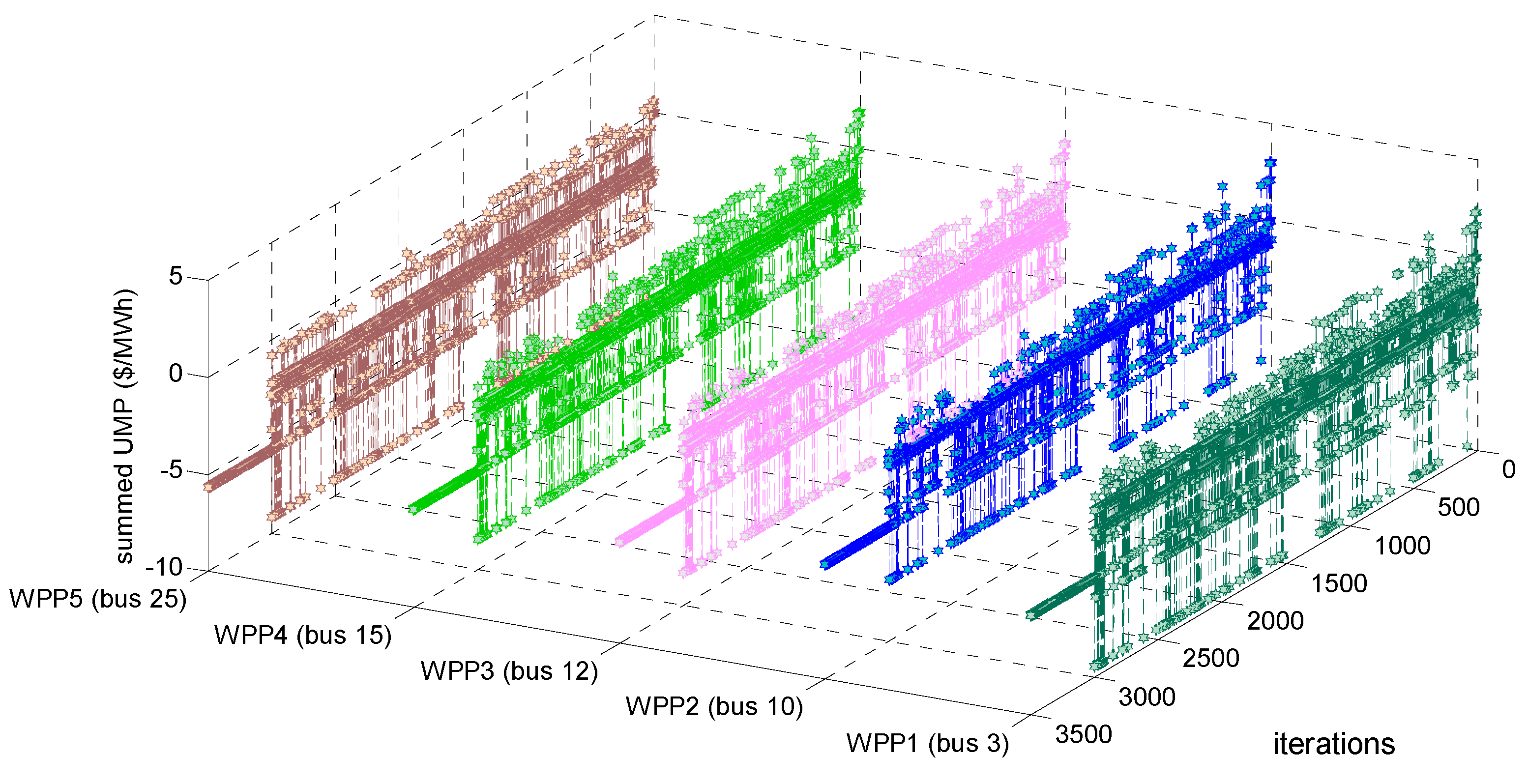
Figure 4. Moreover, Testing and verifying whether our proposed LSCAC-based day-head EM approach under BM 2 reaches to dynamic stability or not after 3000 training iterations can be shown in
Figure 5,
Figure 6 and
Figure 7. In
Figure 4 and
Figure 7, summed UMP at bus
m in each iteration can be calculated by using Equation (39).
Before we analyze BMs and strategies for WPPs by using our proposed LSCAC-based day-head EM modeling approach, it should be tested first whether our proposed approaches under different BMs converge to dynamic stabilities after every WPP experiences enough iterations of on line training. If the convergence was verified, the market state and obtained action of every WPP would no longer change after enough training iterations. It should be noted that in the existing TBRL-based approaches [
26,
27,
28,
29,
30,
31,
36], the action set of every agent is discrete and finite, and the optimality of an agent’s final obtained action can be easily verified by using method mentioned in [
31], which is to compare profits brought from all actions in this agent’s action set while fixing the actions of other agents. However, in our proposed LSCAC-based approach, the action set of every agent is continuous. It is impossible to directly test the optimality of an agent’s final obtained action because there are infinite actions other than this final obtained one. Therefore, we propose the following three steps to further test the performance of the LSCAC-based day-head EM modeling approach:
To test the optimality of a WPP’s final obtained strategy in TBRL-based (i.e., Q-Learning algorithm [
26,
27]) day-head EM modeling approaches after converging to dynamic stabilities by comparing profits brought from all this WPP’s strategies while fixing other WPPs’ obtained strategies. The specific optimality test method can be seen in [
31].
To test whether a WPP can obtain more profit by using LSCAC algorithm than TBRL algorithm (Q-Learning algorithm [
26,
27]) or not, after converging to dynamic stabilities.
To test whether the whole market can reach lower operation cost in our proposed LSCAC-based approach than TBRL-based (Q-Learning algorithm [
26,
27]) one or not, after converging to dynamic stabilities.
The related parameters of our LSCAC-based day-head EM modeling approach are listed in
Table 5.
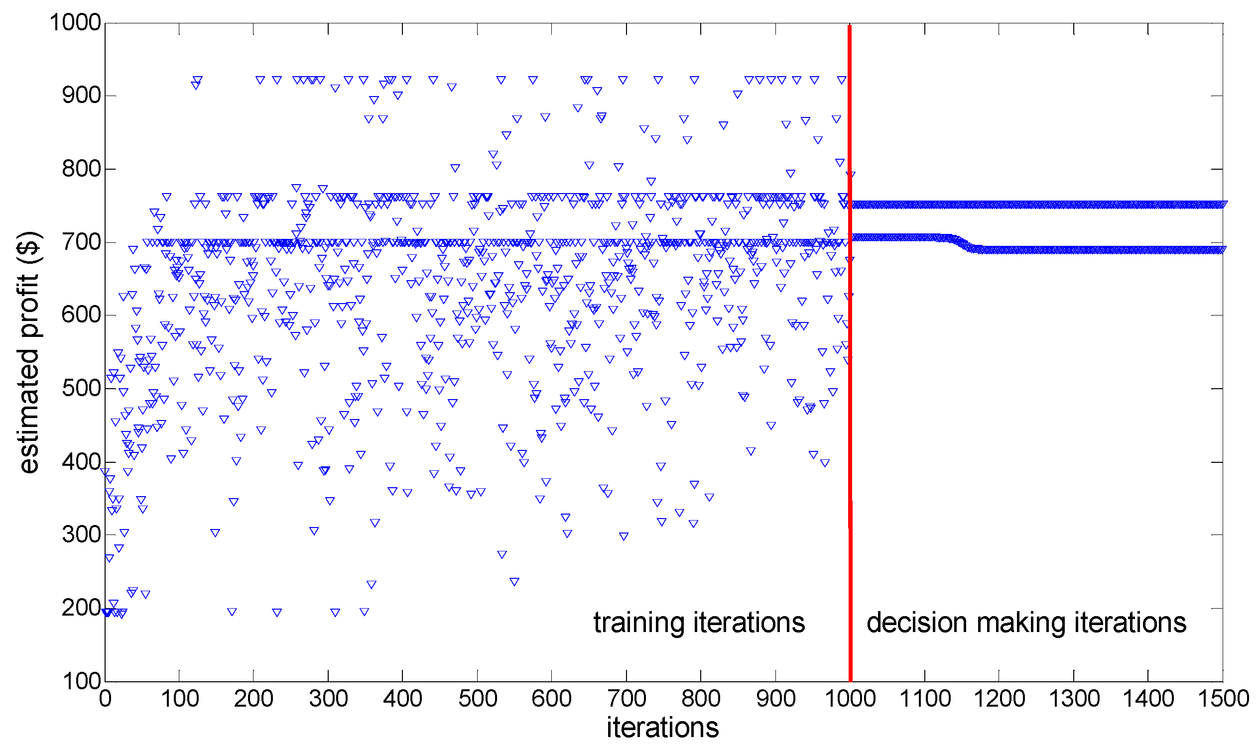
From
Figure 2,
Figure 3 and
Figure 4, it can be seen that, after randomly fluctuating in 3000 training iterations, the adjustment processes of estimated profit, LMP and summed UMP of every WPP remain constant during 500 decision-making iterations. Actually, other adjustment processes such as that of operation cost, every WPP’s bidding strategy, etc. also become constant after 3000 training iterations. Therefore, our proposed approach under BM 1 can converge to dynamic stability after every WPP experiences 3000 iterations of online training.
From
Figure 5,
Figure 6 and
Figure 7, it can be seen that, after randomly fluctuating in 3000 training iterations, the adjustment processes of estimated profit, LMP and summed UMP of every WPP remain constant during 500 decision-making iterations. Actually, other adjustment processes such as that of operation cost, every WPP’s bidding strategy, etc. also become constant after 3000 training iterations. Therefore, our proposed approach under BM 2 can converge to dynamic stability after every WPP experiences 3000 iterations of online training.
The main reason about the fluctuating trends in the 3000 training iterations in
Figure 2,
Figure 3,
Figure 4,
Figure 5,
Figure 6 and
Figure 7 is that in order to balance the exploration and exploitation during these 3000 training iterations, every WPP must maintain the ability of exploration which is to randomly select bidding strategies according to the repeatedly updated Equation (45), all WPPs’ insufficient experiences and unstable action selecting policies make the dynamic training process of EM fluctuate randomly. The main reason about the constant trends in 500 decision-making iterations in
Figure 2,
Figure 3,
Figure 4,
Figure 5,
Figure 6 and
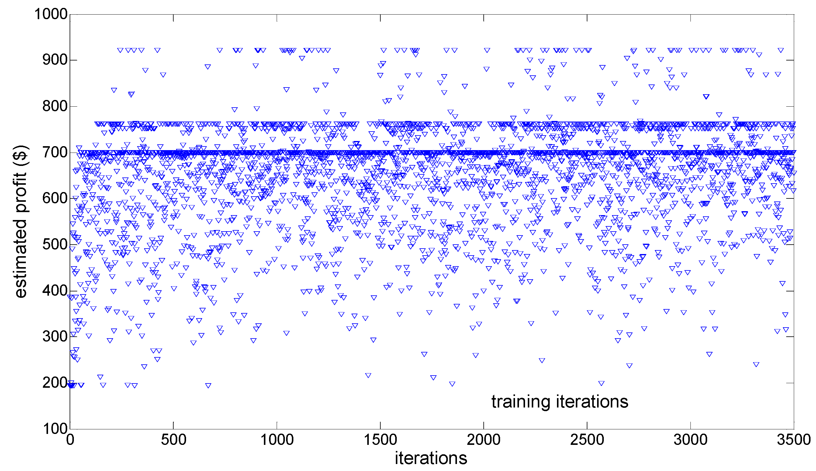
Figure 7 is that after accumulating enough experiences, every WPP adopts the greedy policy which is to only select its considered optimal bidding strategy in face of any observed EM state in each of the 500 decision-making iterations, all WPPs’ sufficient experiences and stable action selecting policies make the dynamic decision-making process of EM converge to stability. Therefore, it may be concluded that enough training iterations considering the balance of exploration and exploitation, as well as the greedy action selecting policy adopted in decision-making iterations are two main factors resulting in EM dynamic stability. Taking EM approach under BM 1 for example,
Figure 8 shows the dynamic adjusting process of WPP
1’s estimated profit when every WPP experiences 1000 training iterations and 500 decision-making iterations, and
Figure 9 shows the dynamic adjustment process of WPP
1’s estimated profit when every WPP experiences 3500 training iterations without greedy action selecting policy.
From
Figure 8, it is shown that although the greedy action selecting policies are adopted by WPPs in decision-making iterations, insufficient training iterations, which mean insufficient experiences accumulated, still make WPP
1’s estimated profit fluctuate during decision-making process. Actually, the dynamic adjustment processes of other WPPs’ estimated profits also fluctuate during decision-making iterations.
From
Figure 9, it is shown that although more than 3000 training iterations considering the balance of exploration and exploitation are conducted, WPP
1’s estimated profit still fluctuates during the last 500 iterations due to its lack of a greedy action selection policy. Actually, the dynamic adjustment processes of other WPPs’ estimated profits also fluctuate during the last 500 iterations. Moreover, WPP
1’s estimated profit in
Figure 9 is much more volatile during the last 500 iterations than that in
Figure 8, which is mainly because WPPs lacking greedy action selection policies tend to bid more randomly in the EM.
Therefore, EM dynamic stability cannot be reached whether there are insufficient training iterations or the greedy action selecting policy is not considered, which, to a certain extent, on the one hand verifies our conclusions about the two main factors resulting in EM dynamic stability, and on the other hand, suggests that the proposed 3000 training iterations and 500 decision-making iterations are comparatively reasonable for our proposed LSCAC-based approach to reach EM dynamic stability.
To further test the performance of our proposed approaches under different BMs, two Q-learning-based day-ahead EM approaches (QDEMAs) are taken for comparison. In these QDEMAs, some WPPs are designated as Q-learning-based agents while other undesignated WPPs are still the LSCAC-based ones. A Q-learning-based agent dynamically adjusts its action based on Q-learning algorithm which use
ε-greedy policy [
26] to balance exploration and exploitation in 3000 training iterations, and greedy policy in 500 decision-making iterations. Difference among these QDEMAs is only reflected in the number of Q-learning-based agents. Parameters related to these two QDEMAs are listed in
Table 6.
After 3000 training and 500 decision-making iterations, the obtained market results of those two QDEMAs and our proposed approach under BM 1 are listed in
Table 7, and the obtained results of those two QDEMAs and our proposed approach under BM 2 are listed in
Table 8. Moreover, like our proposed LSCAC-based approach, no matter under which BM, both these QDEMAs can converge to dynamic stability after every WPP experiences 3000 iterations of online training. That means those results listed in
Table 7 and
Table 8 are not obtained accidentally, a LSCAC-based or Q-learning-based WPP does not change its strategy when market state affected by all WPPs’ strategies keeps unchanged.
By using the optimality test method in [
31], no matter under which BM and in which QDEMA, every Q-learning-based WPP’s final obtained strategy can be verified as its optimal one in its discrete action set, which can bring it the most profit when other WPPs’ strategies are fixed.
No matter under which BM, on the one hand, estimated profits of WPP1 and WPP2 in QDEMA 2 are higher than those in QDEMA 1, respectively, and estimated profits of WPP3, WPP4 and WPP5 in our proposed LSCAC-based approach are higher than those in QDEMA 2, respectively, which, to some extent, indicates one can get more profit by using the LSCAC algorithm to bid in EM than the Q-learning one within the same conditions; on the other hand, the operation cost in our proposed LSCAC-based approach is lower than that in QDEMA 2, and the operation cost in QDEMA 2 is lower than that in QDEMA 1, which, to some extent, indicates that with the increase in the number of LSCAC-based agents in EM, the operation cost of whole system can be reduced.
In conclusion, no matter under which BM, Q-learning-based WPPs can finally find their optimal bidding strategies from their discrete and finite action sets. If these WPPs are transformed into LSCAC-based ones, they can finally find their more applicable strategies from their continuous action sets, which not only bring more profits for themselves but also bring lower operation cost for the whole system than that based on Q-learning method. Hence, although it is hard to directly test the optimality of every LSCAC-based WPP’s final obtained strategy, our further test has, to some extent, verified the rationality and scientific basis of applying our proposed LSCAC-based approach in day-ahead EM modeling for strategic WPPs.
Moreover, no matter under which BM, simulation of our proposed approach on IEEE 30 bus test system with five strategic WPPs takes only about 43 seconds to reach the final results (after 3500 iterations). That is to say, the time complexity of our proposed approach is relatively low so that we can extend it to the modeling and simulation of more realistic and more complex EM system.
4.4. BMs Analysis for WPPs
In this section, our proposed LSCAC-based approach is applied to analyze the obtained market results under different BMs after 3000 training iterations and 500 decision-making iterations.
Moreover, it should be noted that under BM 2, in order to lead WPPi() to reasonably bid in market, we set lower and upper limits and ($/MWh) for its bidding price . Values of and () may affect the obtained market results such as final obtained LMPs, estimated profits of all WPPs and operation cost of the system etc. after 3500 iterations. Hence, different values of and () should be taken into account when considering BMs. For the sake of simplicity and without losing generality, we set , and different values of and are considered.
After 3500 iterations, considering different values of
(while fixing the upper limit
to 50
$/MWh, the same as what listed in
Table 5,
Table 9 is listed for the comparison of obtained market results under different BMs.
After 3500 iterations, considering different values of
(while fixing the upper limit
to 30
$/MWh, the same as what was listed in
Table 5,
Table 10 is provided for the comparison of obtained market results under different BMs.
In
Table 9, when values of
are 0, 10, 20 and 30 (
$/MWh), respectively, the obtained profit of every WPP, operation cost and average LMP of 30 buses under BM 2 remain unchanged. Actually, if
≤ 30
$/MWh, the obtained bidding price (strategy) of every WPP under BM 2 is higher than 30 (
$/MWh), which means values of
lower than 30 (
$/MWh) cannot affect every WPP’s bidding decision-making. Therefore, in our opinion, it is hard to weaken the market power of every WPP by only reducing the value of lower limit of every WPP’s bidding price while WPPs provide ISO their bidding curves consisting of bidding prices and power outputs for the next day.
In
Table 10, the obtained profit of every WPP, operation cost and average LMP of 30 buses under BM 2 increases with the increase of the value of
. That may be mainly because the more the value of
is, the greater market power WPPs have. Therefore, in our opinion, the upper limit of every WPP’s bidding price should not be set too high while WPPs provide ISO their bidding curves consisting of bidding prices and power outputs for the next day.
In most cases of and , WPPs under BM 2 can get more profits than under BM 1, which may be because WPPs under BM 2 can obtain greater market power by directly adjusting their bidding prices so as to further improve their profits compared with WPPs under BM 1. However, from the perspective of the whole market, both the obtained operation cost and average LMP under BM 2 are higher than that under BM 1, which, to some extent, indicates WPPs adopting BM 2 cause lower economic efficiency in the whole market than adopting BM 1. Therefore, in our opinion, if the purpose of permitting WPPs to bid is to promote the development of wind power resources by improving WPPs’ profits, providing ISO their bidding curves is more applicable, and if the purpose of permitting WPPs to bid is to improve the economic efficiency of the whole market, only sending their power output plans is more applicable.


