
Applicability of an Artificial Neural Network for Predicting Water-Alternating-CO2 Performance


Abstract
1. Introduction
2. 3D Model Characteristics
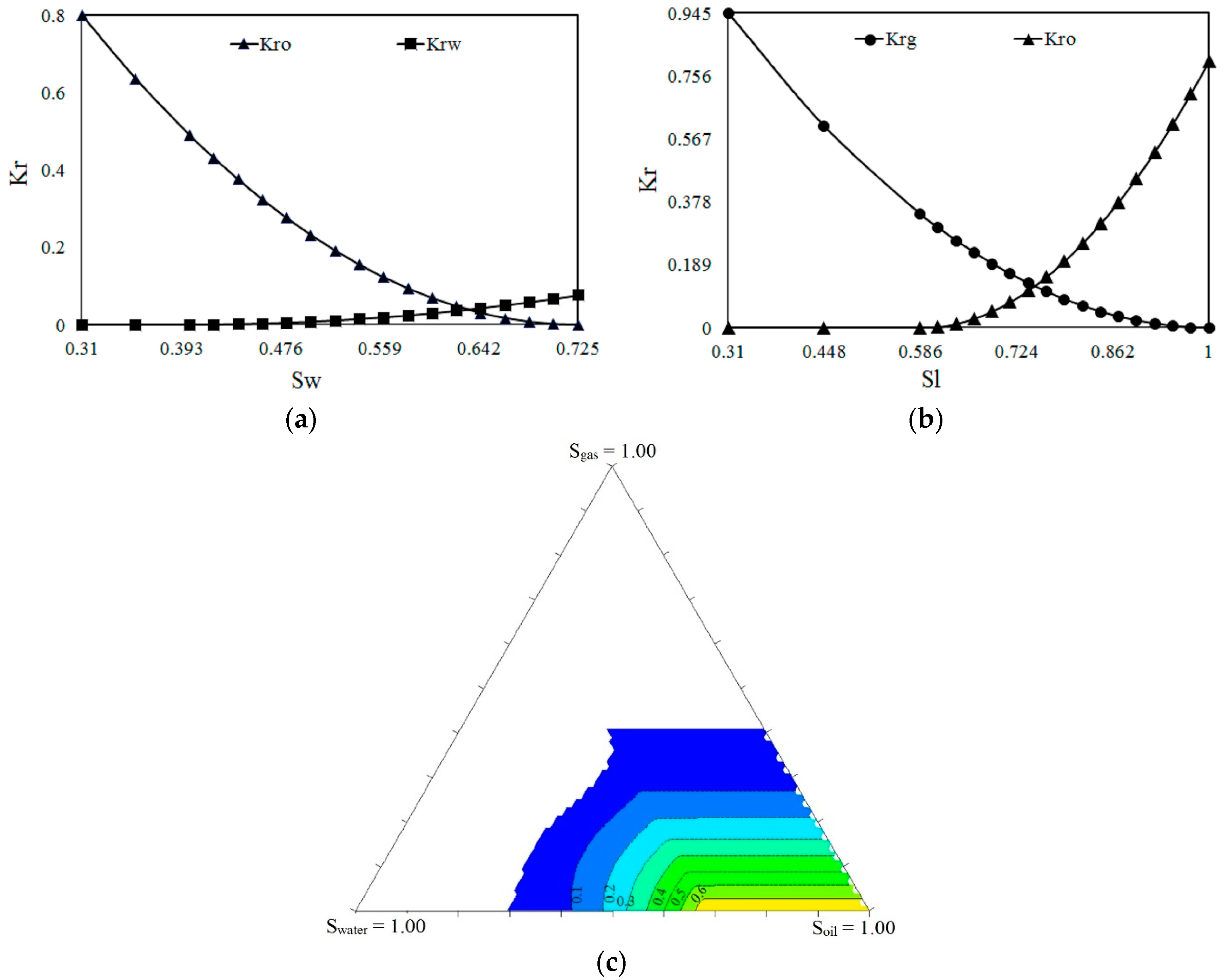
2.1. Reservoir Descriptions
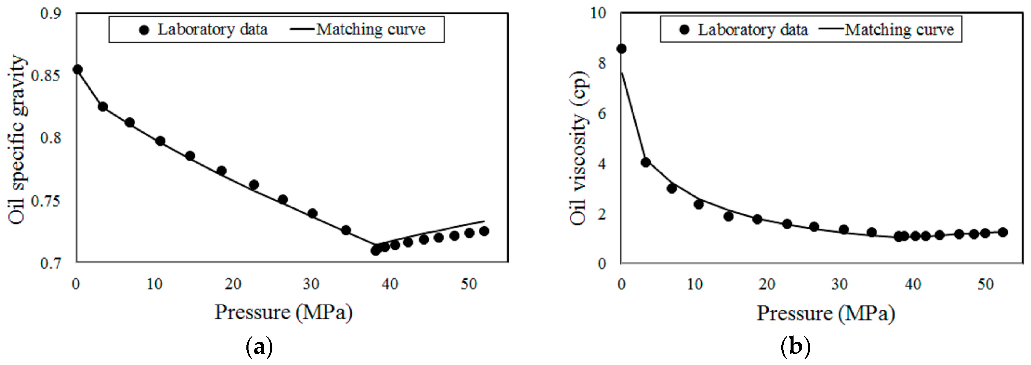
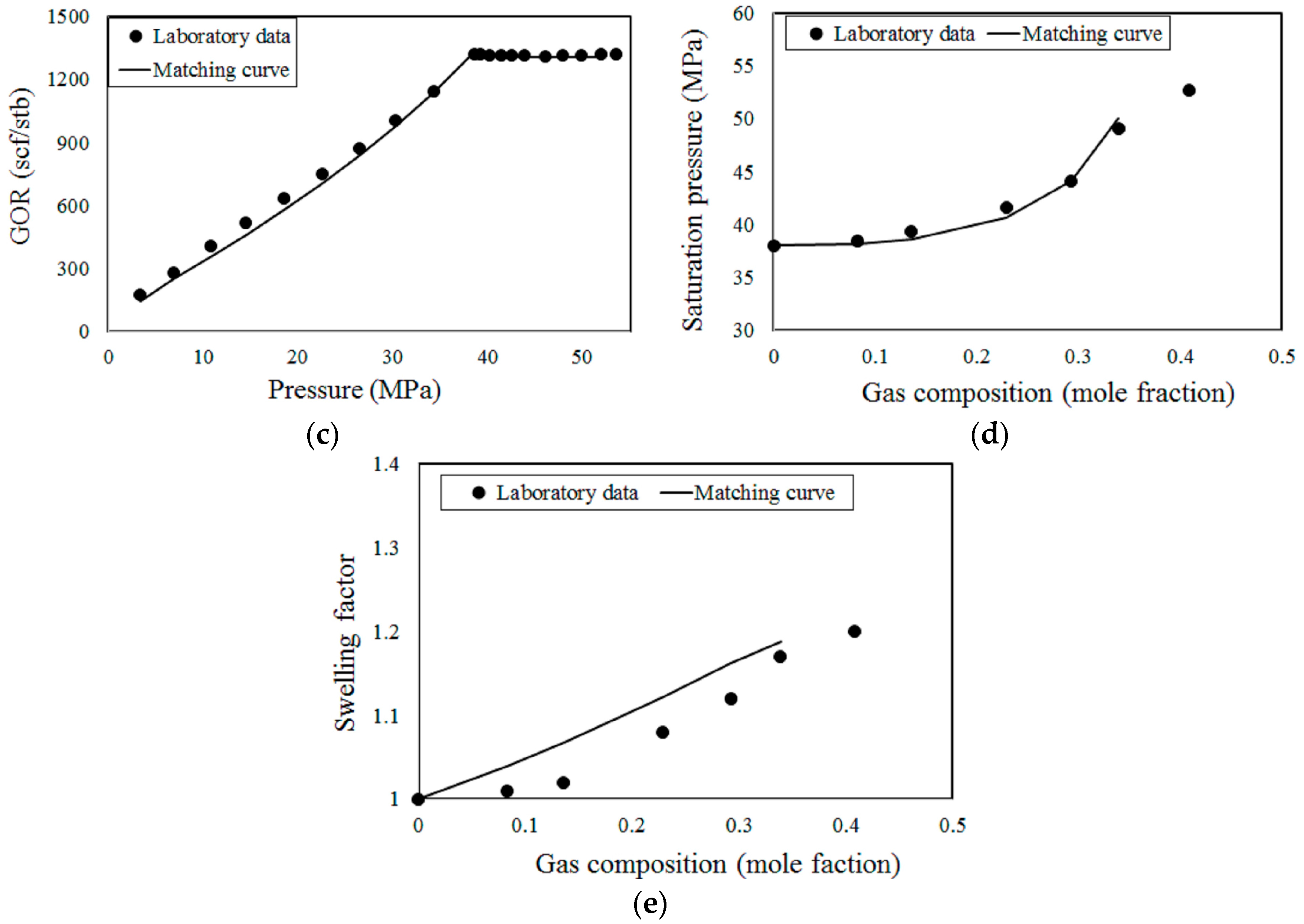
2.2. Fluid Properties
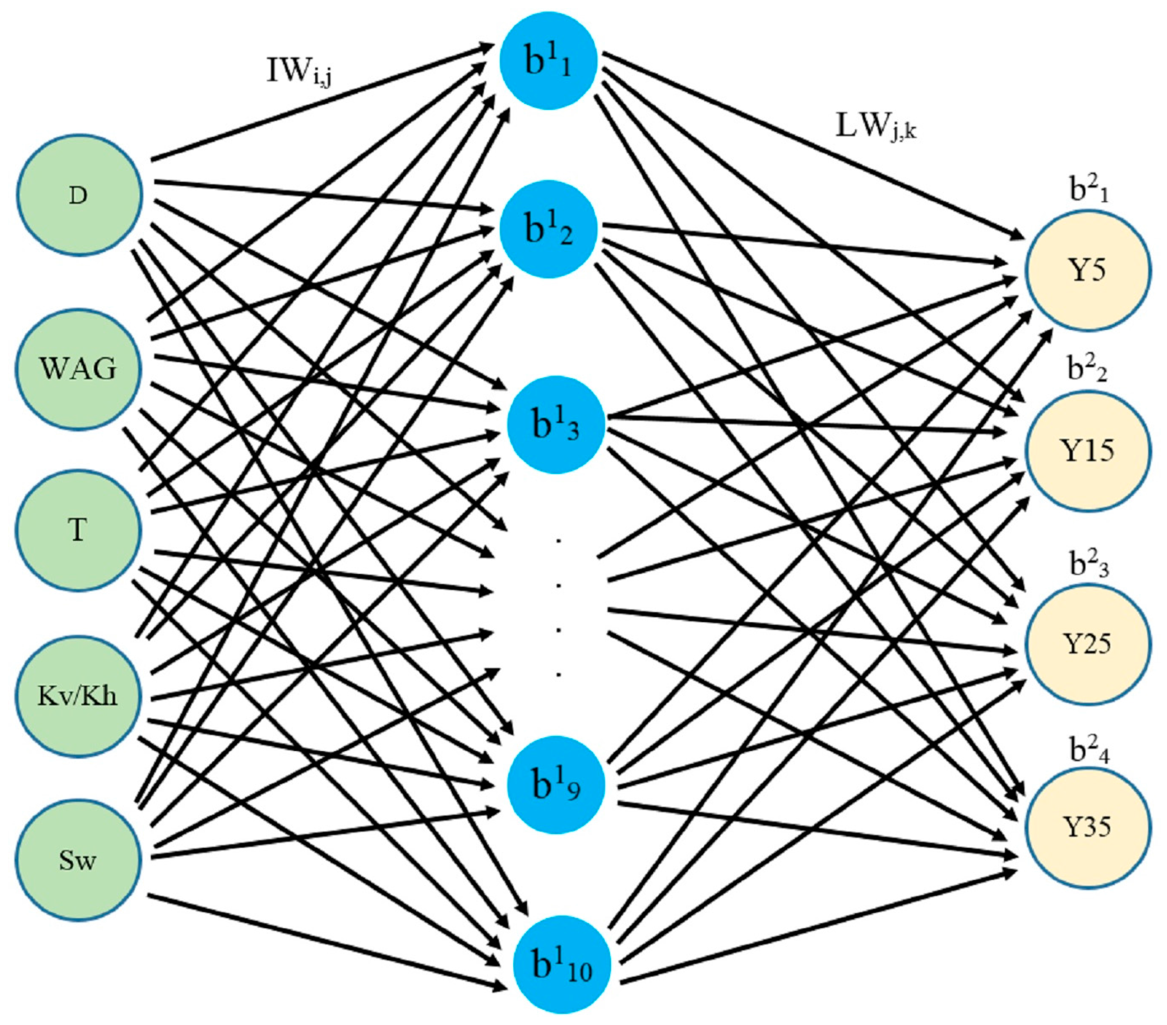
3. Neural Network Model Generation
4. Results and Discussion
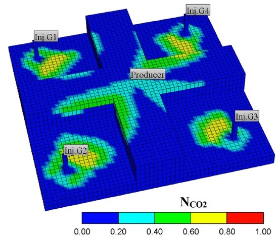
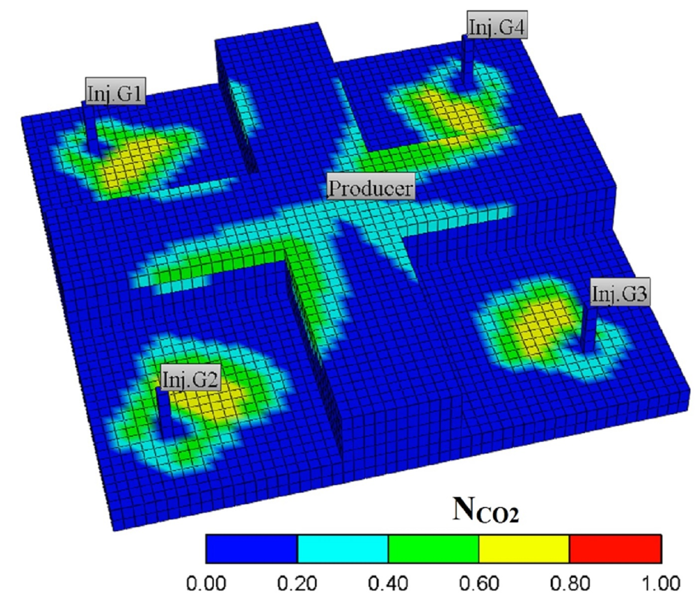
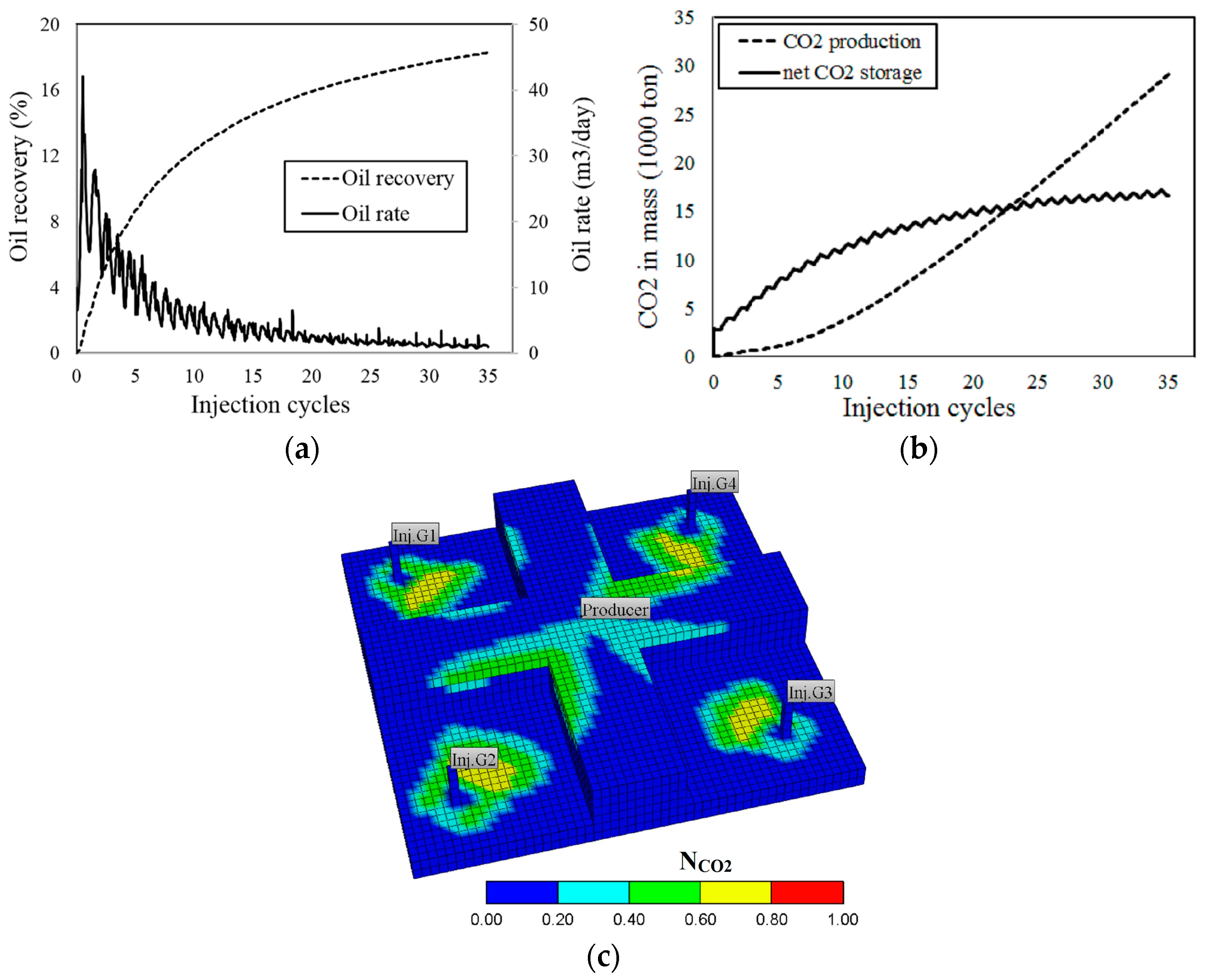
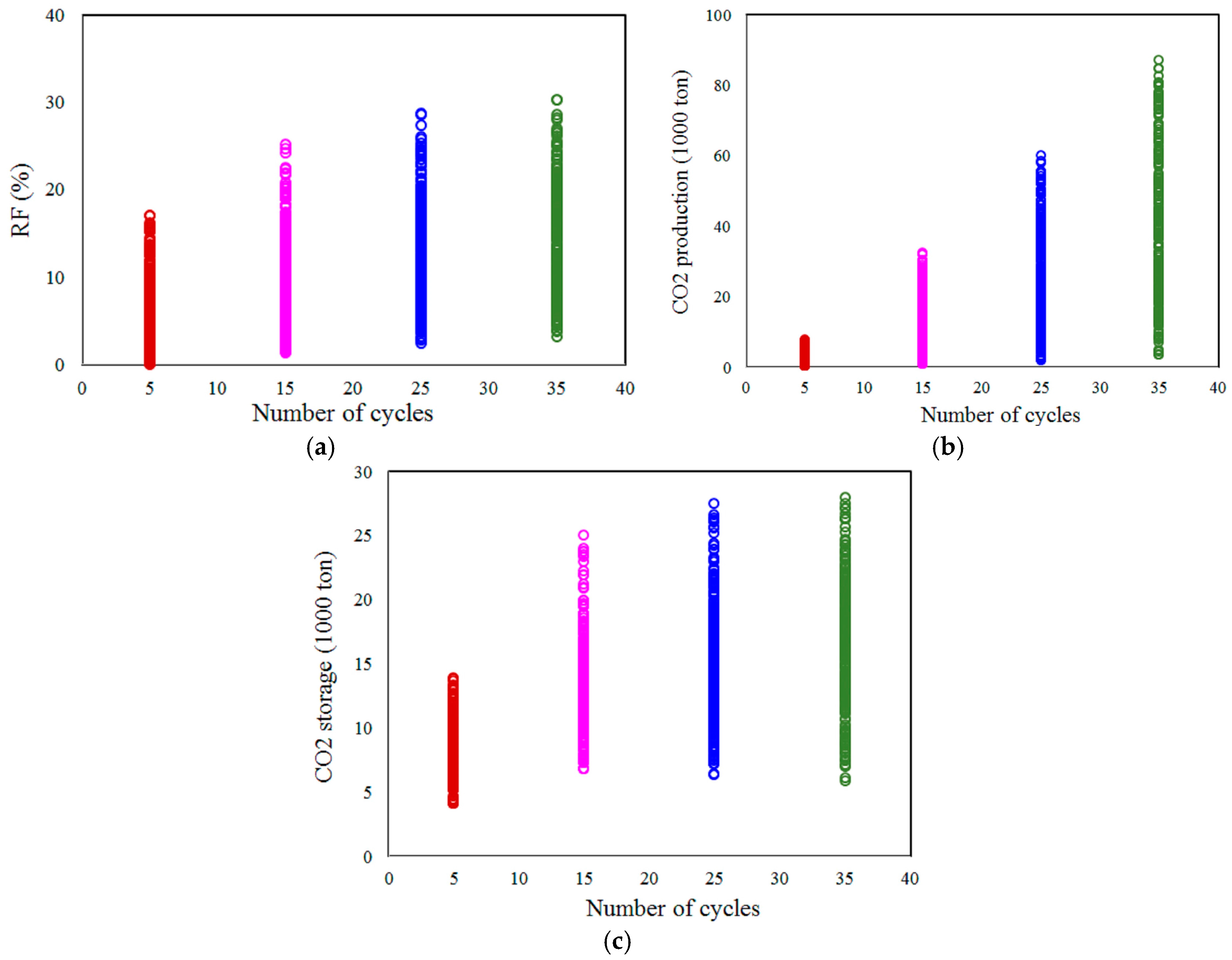
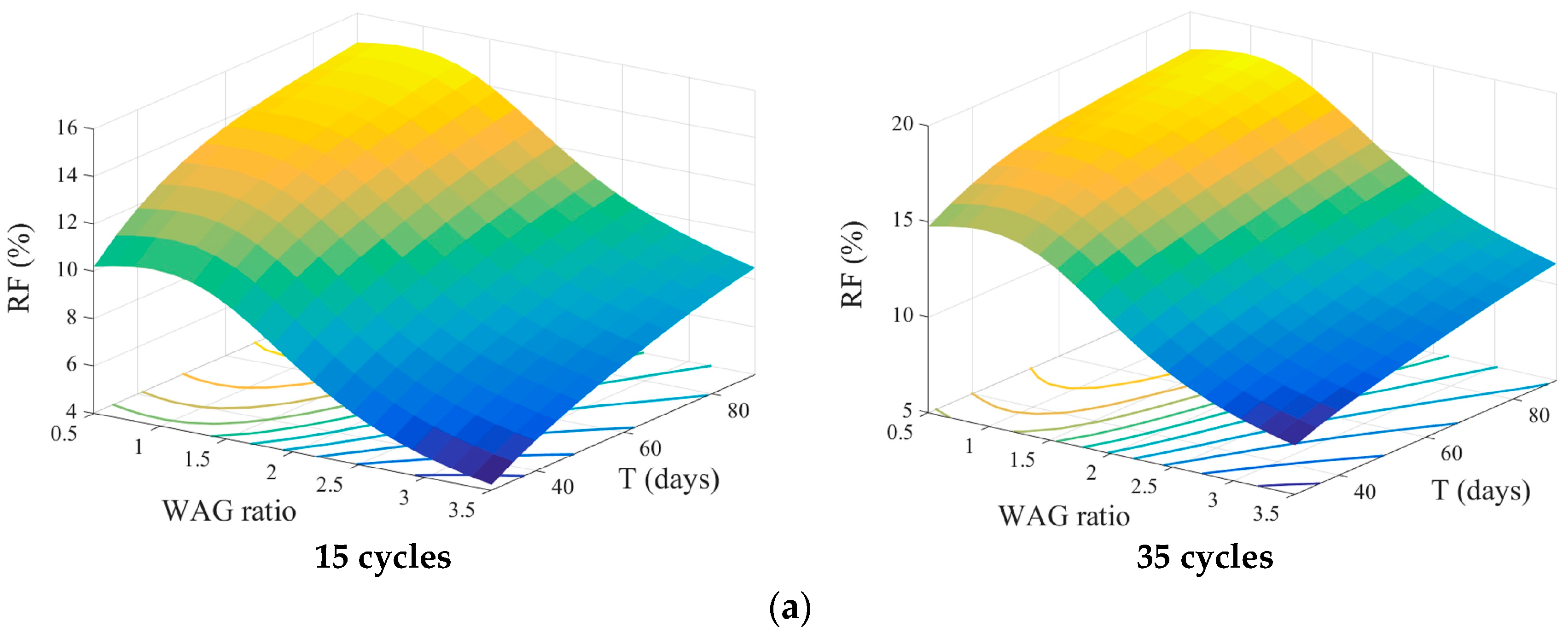
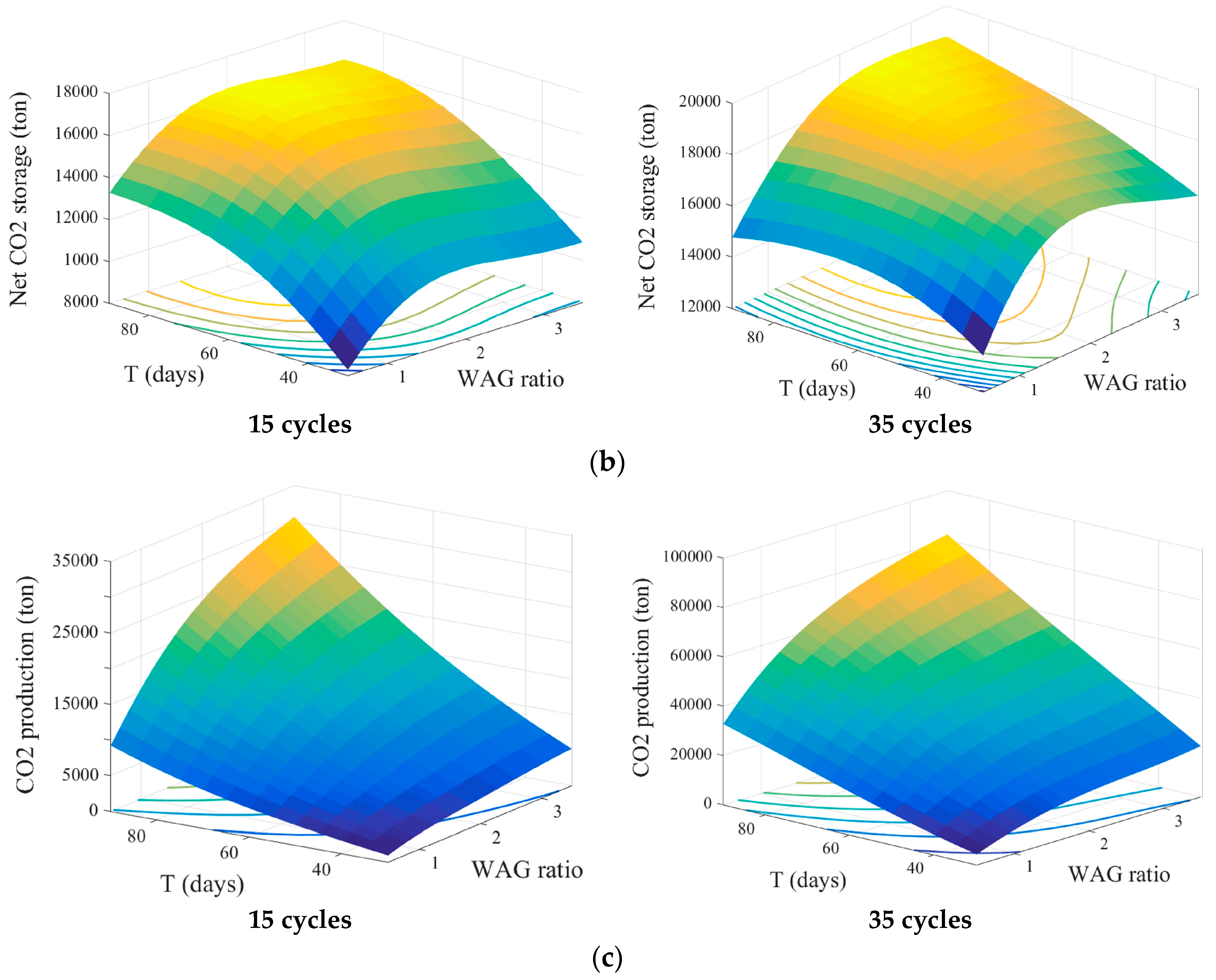
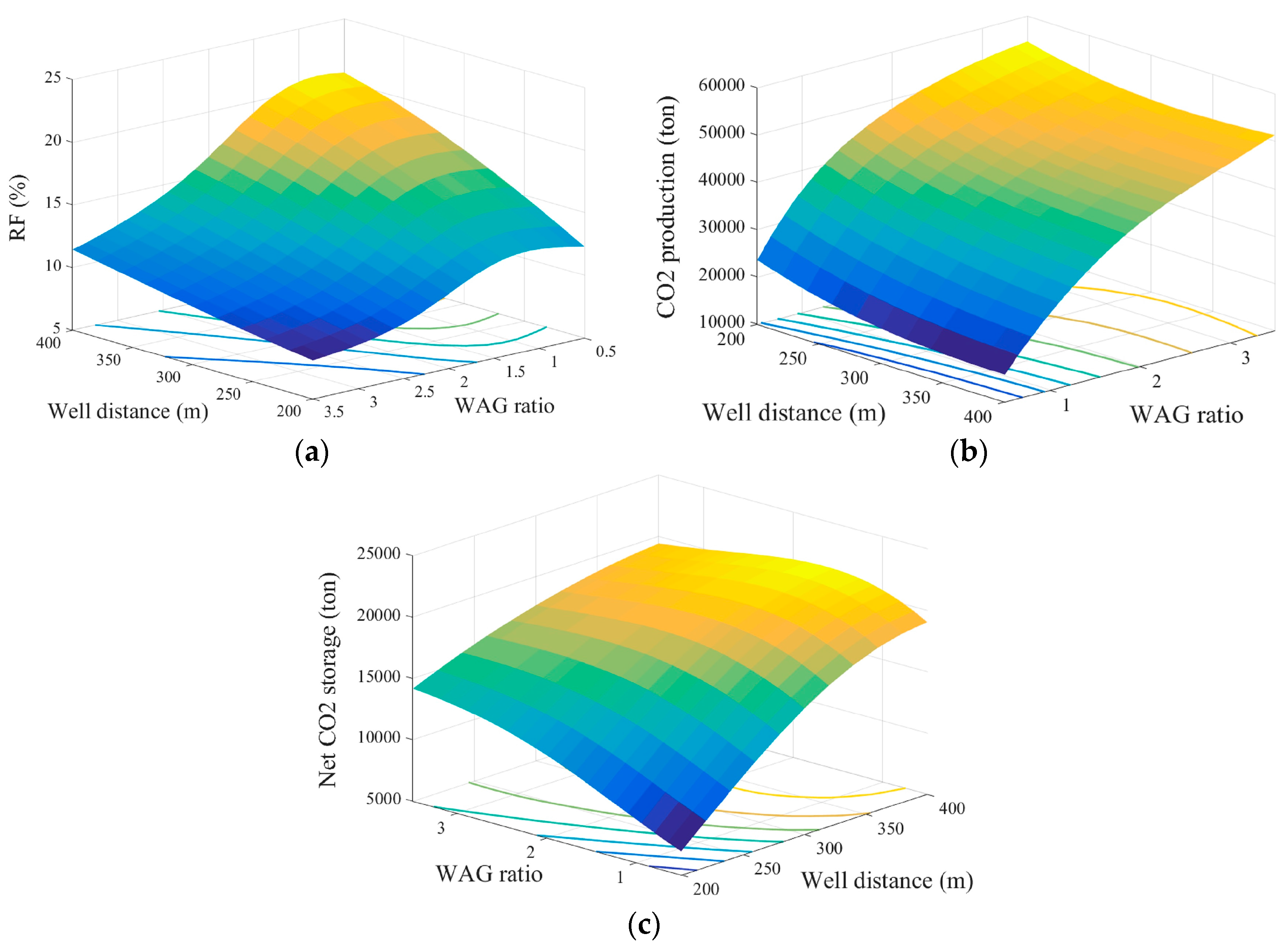
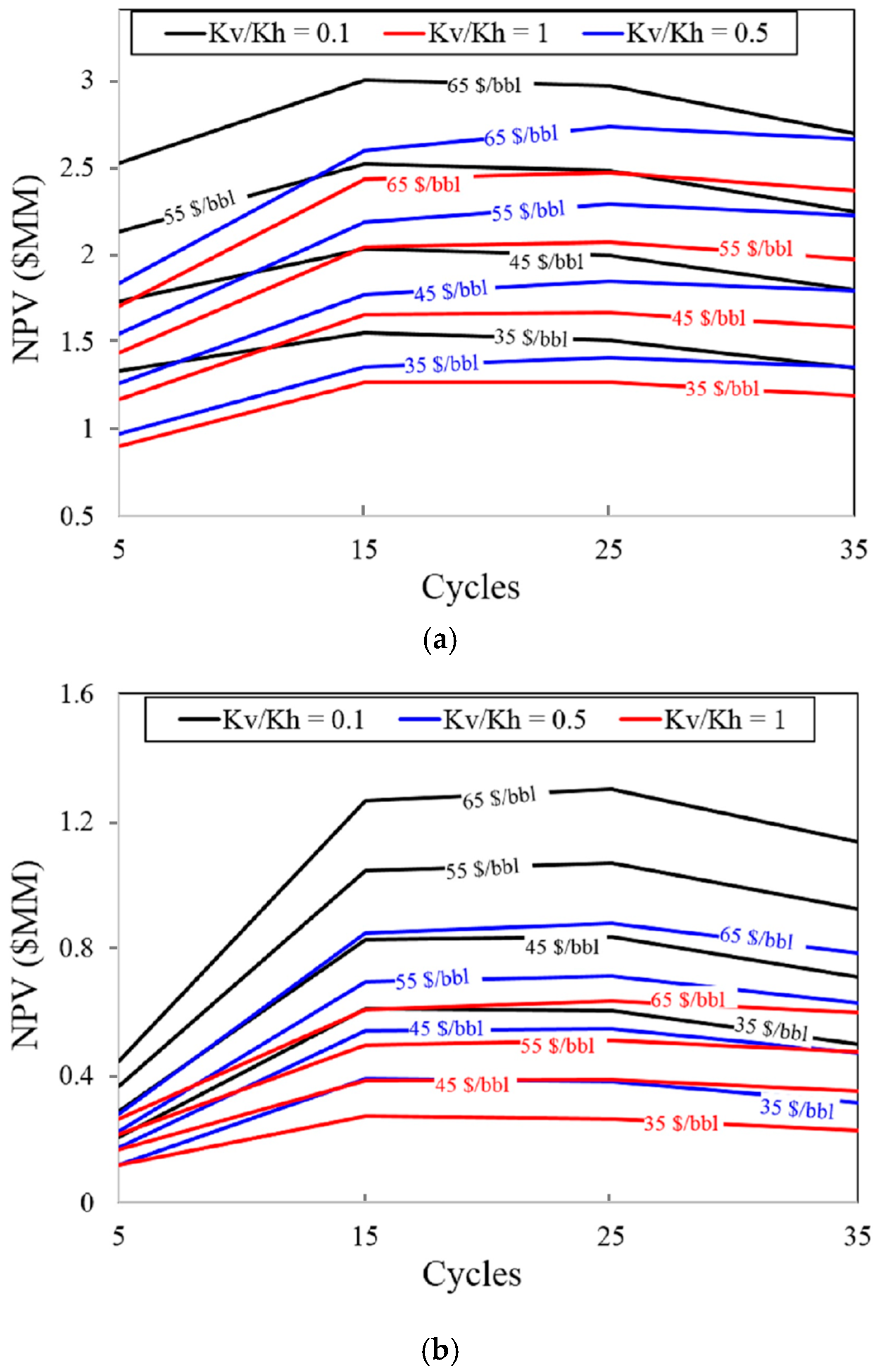
4.1. Simulation Results
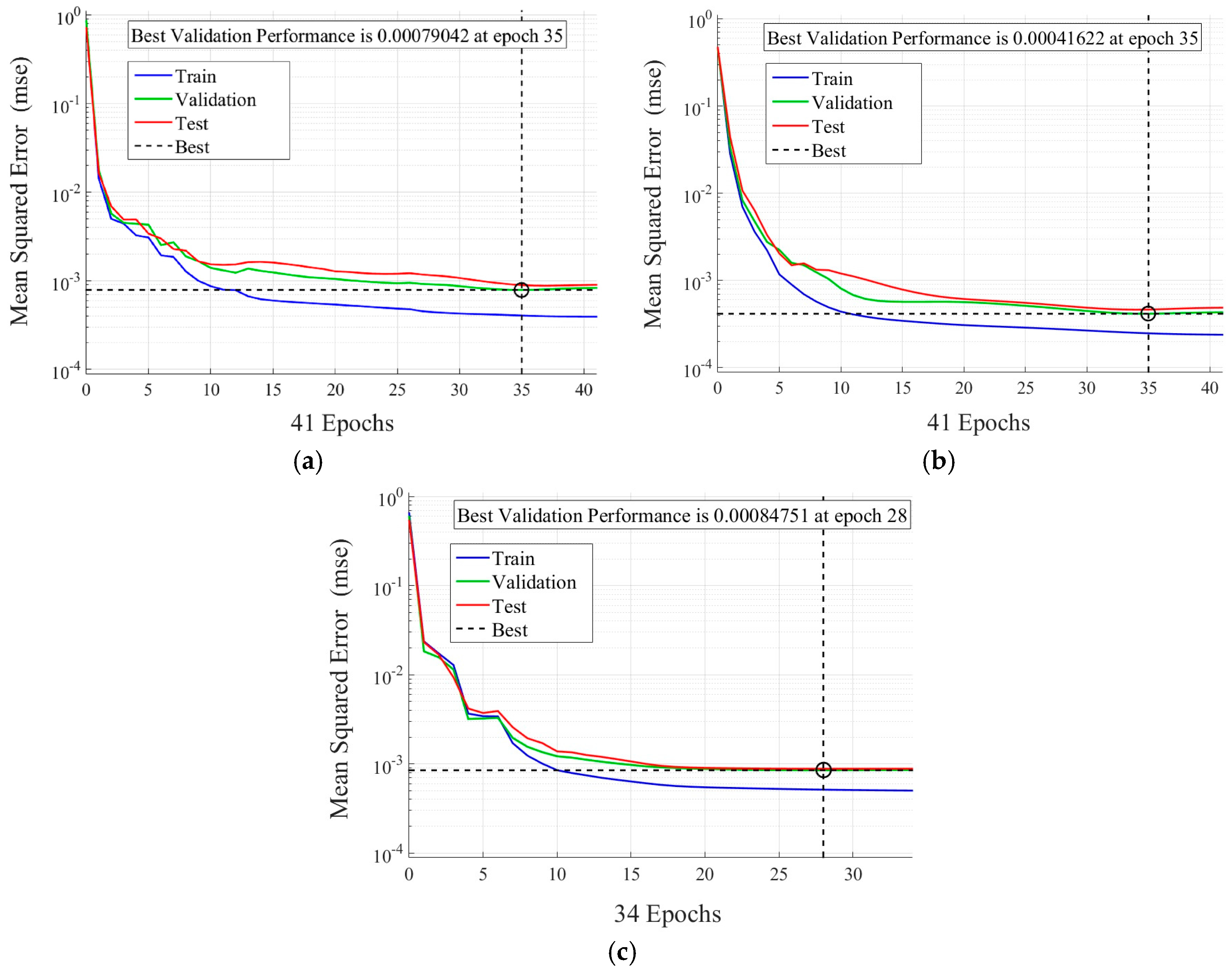
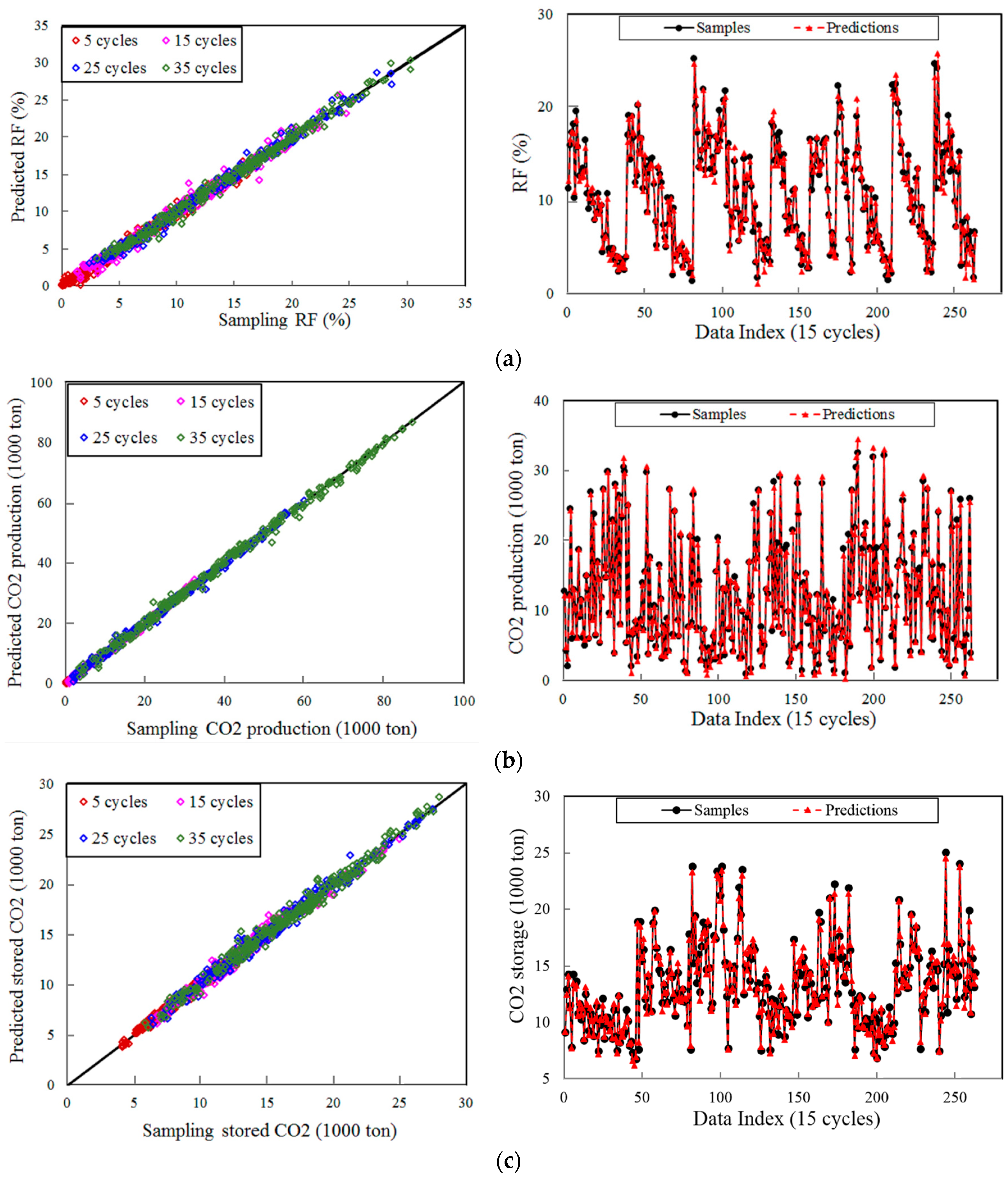
4.2. Neural Network Model Evaluations
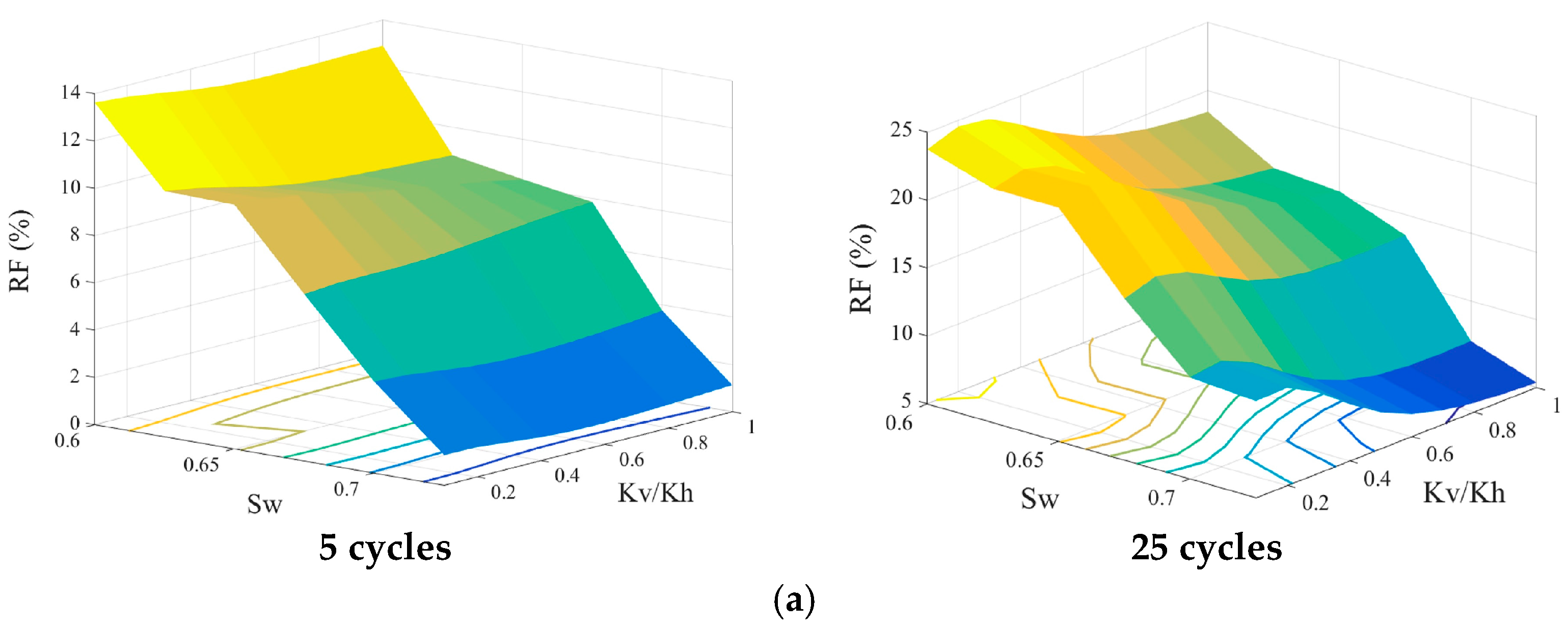
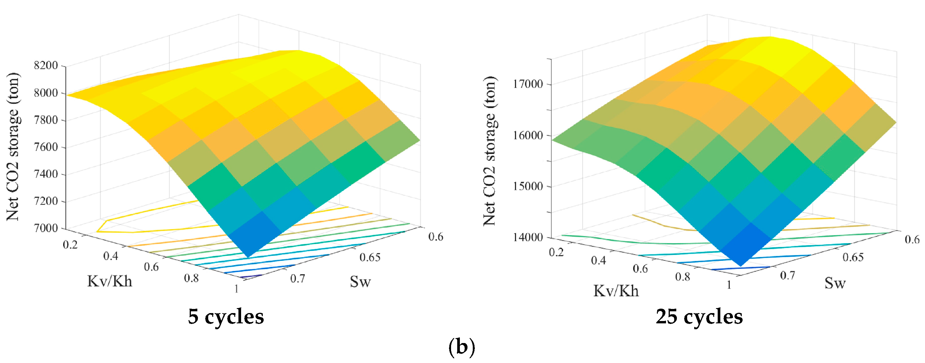
4.3. Applicability of ANN Models
5. Conclusions
Author Contributions
Conflicts of Interest
References
- Perera, M.S.A.; Gamage, R.P.; Rathaweera, T.D.; Ranathunga, A.S.; Koay, A.; Choi, X. A review of CO2-Enhaced oil recovery with a simulated sensitivity analysis. Energies 2016, 9, 481. [Google Scholar] [CrossRef]
- Si, L.V.; Chon, B.H. Artificial neural network model for alkali-surfactant-polymer flooding in viscous oil reservoirs: Generation and application. Energies 2016, 9, 1081. [Google Scholar]
- Zaluski, W.; El-Kaseeh, G.; Lee, S.Y.; Piercey, M.; Duguid, A. Monitoring technology ranking methodology for CO2-EOR sites using the Weyburn-Midale field as a case study. Int. J. Greenh. Gas Control 2016, 54, 466–478. [Google Scholar] [CrossRef]
- Nobakht, M.; Moghadam, S.; Gu, Y. Effects of viscous and capillary forces on CO2 enhanced oil recovery under reservoir conditions. Energy Fuels 2007, 21, 3469–3476. [Google Scholar] [CrossRef]
- Zanganeh, P.; Ayatollahi, S.; Alamdari, A.; Zolghadr, A.; Dashti, H.; Kord, S. Asphaltene deposition during CO2 injection and pressure depletion: A visual study. Energy Fuels 2012, 26, 1412–1419. [Google Scholar] [CrossRef]
- Ping, H.L.; Ping, S.P.; Wei, L.X.; Chao, G.Q.; Sheng, W.C.; Fangfang, L. Study on CO2 EOR and its geological sequestration potential in oil field around Yulin city. J. Petrol. Sci. Eng. 2015, 134, 199–204. [Google Scholar] [CrossRef]
- Ampomah, W.; Balch, R.S.; Grigg, R.B.; Will, R.; Dai, Z.; White, M.D. Farnsworth field CO2-EOR project: Performance case history. In Proceedings of the SPE Improved Oil Recovery Conference, Tulsa, OK, USA, 11–13 April 2016. [Google Scholar]
- Ren, B.; Ren, S.; Zhang, L.; Chen, G.; Zhang, H. Monitoring on CO2 migration in a tight oil reservoir during CCS-EOR in Jilin oilfield China. Energy 2016, 98, 108–121. [Google Scholar] [CrossRef]
- Raza, A.; Rezaee, R.; Gholami, R.; Bing, C.H.; Nagarajan, R.; Hamid, M.A. A screening criterion for selection of suitable CO2 storage sites. J. Nat. Gas Sci. Eng. 2016, 28, 317–327. [Google Scholar] [CrossRef]
- Ahmadi, M.A.; Pouladim, B.; Barghi, T. Numerical modeling of CO2 injection scenarios in petroleum reservoirs: Application to CO2 sequestration and EOR. J. Nat. Gas Sci. Eng. 2016, 30, 38–49. [Google Scholar] [CrossRef]
- He, L.; Shen, P.; Liao, X.; Li, F.; Gao, Q.; Wang, Z. Potential evaluation of CO2 EOR and sequestration in Yanchang oilfield. J. Energy Inst. 2016, 89, 215–221. [Google Scholar] [CrossRef]
- Teklu, T.W.; Alameri, W.; Graves, R.; Kazemi, H. Low-salinity water-alternating-CO2 EOR. J. Petrol. Sci. Eng. 2016, 142, 101–118. [Google Scholar] [CrossRef]
- Yao, Y.; Wang, Z.; Li, G.; Wu, H.; Wang, J. Potential of carbon dioxide miscible injections into the H-26 reservoir. J. Nat. Gas Sci. Eng. 2016, 34, 1085–1095. [Google Scholar] [CrossRef]
- Song, Z.; Li, Z.; Wei, Z.; Lai, F.; Bai, B. Sensitivity analysis of water-alternating-CO2 flooding for enhanced oil recovery in high water cut oil reservoirs. Comput. Fluids 2014, 99, 93–103. [Google Scholar] [CrossRef]
- Wei, N.; Li, X.; Dahowski, R.T.; Davidson, C.L. Economic evaluation on CO2-EOR of onshore oil fields in China. Int. J. Greenh. Gas Control 2015, 37, 170–181. [Google Scholar] [CrossRef]
- Ettehadtavakkol, A.; Lake, L.W.; Bryant, S.L. CO2-EOR ans storage design optimization. Int. J. Greenh. Gas Control 2014, 25, 79–92. [Google Scholar] [CrossRef]
- Ahmadi, M.A. Neural network based unified particle swarm optimization for prediction of asphaltene precipitation. Fluid Phase Equilibr. 2012, 314, 46–51. [Google Scholar] [CrossRef]
- Pan, F.; McPherson, B.J.; Daim, Z.; Lee, S.Y.; Ampomah, W.; Viswanathan, H.; Esser, R. Uncertainty analysis of carbon sequestration in an active CO2-EOR field. Int. J. Greenh. Gas Control 2016, 51, 18–28. [Google Scholar] [CrossRef]
- Dai, Z.; Viswanathan, H.; Middleton, R.; Pan, F.; Ampomah, W.; Yang, C.; Jia, W.; Lee, S.Y.; Balch, R.; Grigg, R.; White, M. CO2 accounting and risk analysis for CO2 sequestration at enhanced oil recovery sites. Environ. Sci. Technol. 2016, 50, 7546–7554. [Google Scholar] [CrossRef] [PubMed]
- Eshraghi, S.E.; Rasaeim, M.R.; Zendehboudi, S.Z. Optimization of miscible CO2 EOR and storage using heuristic methods combined with capacitance/resistance and Gentil fractional flow models. J. Nat. Gas Sci. Eng. 2016, 32, 304–318. [Google Scholar] [CrossRef]
- Ampomah, W.; Balch, R.; Cather, M.; Coss, D.R.; Dai, Z.; Heath, J.; Dewers, T.; Mozley, P. Evaluation of CO2 storage mechanisms in CO2 enhanced oil recovery sites: Application to Morrow sandstone reservoir. Energy Fuels 2016, 30, 8545–8555. [Google Scholar] [CrossRef]
- Li, L.; Khorsandi, S.; Johns, R.T.; Dilmore, R.M. CO2 enhanced oil recovery and storage using a gravity-enhanced process. Int. J. Greenh. Gas Control 2015, 42, 502–515. [Google Scholar] [CrossRef]
- Moortgat, J.; Firoozabadi, A.; Li, Z.; Esposito, R. Experimental coreflooding and numerial modeling of CO2 injection with gravity and diffusion effects. In Proceedings of the SPE Annual Technical Conference and Exhibition, Florence, Italy, 19–22 September 2010. [Google Scholar]
- Computer Modelling Group Ltd. WINPROP User Guide; Computer Modelling Group Ltd.: Calgary, AB, Canada, 2016. [Google Scholar]
- Orr, F.M.; Dindoruk, B.; Johns, R.T. Theory of multicomponent gas/oil displacements. Ind. Eng. Chem. Res. 1995, 34, 2661–2669. [Google Scholar] [CrossRef]
- Orr, F.M.; Silva, M.K. Effect of oil composition on minimum miscibility pressure-Part 2: Correlation. SPE J. 1987, 2, 479–491. [Google Scholar] [CrossRef]
- Ahmadi, K.; Johns, R.T. Multiple-mixing-cell method for MMP calculations. SPE J. 2011, 16, 733–742. [Google Scholar] [CrossRef]
- Haghtalab, A.; Moghaddam, A.K. Prediction of minimum miscibility pressure using the UNIFAC group contribution activity coefficient model and the LCVM mixing rule. Ind. Eng. Chem. Res. 2016, 55, 2840–2851. [Google Scholar] [CrossRef]
- Damico, J.R.; Monson, C.C.; Frailey, S.; Lasemi, Y.; Webb, N.D.; Grigsby, N.; Yang, F.; Berger, P. Strategies for advancing CO2 EOR in the Illinois Basin, USA. Energy Procedia 2014, 63, 7694–7708. [Google Scholar] [CrossRef]
- Dai, Z.; Middleton, R.; Viswanathan, H.; Rahn, J.F.; Bauman, J.; Pawar, R.; Lee, S.Y.; McPherson, B. An integrated framework for optimizing CO2 sequestration and enhanced oil recovery. Environ. Sci. Technol. Lett. 2014, 1, 49–54. [Google Scholar] [CrossRef]
- Holt, T.; Lindeberg, E.; Berg, D.W. EOR and CO2 disposal-Economic and capacity potential in the North Sea. Energy Procedia 2009, 1, 4159–4166. [Google Scholar] [CrossRef]
- Zhao, X.; Liao, X. Evaluation method of CO2 sequestration and enhanced oil recovery in an oil reservoir, as applied to the Changqing oil fields, China. Energy Fuels 2012, 26, 5350–5354. [Google Scholar] [CrossRef]
- Attavitkamthorn, V.; Vilcaez, J.; Sato, K. Integrated CCS aspect into CO2 EOR project under wide range of reservoir properties and operating conditions. Energy Procedia 2013, 37, 6901–6908. [Google Scholar] [CrossRef][Green Version]
- Gong, Y.; Gu, Y. Miscible CO2 simultaneous water-and-gas (CO2-SWAG) injection in the Bakken formation. Energy Fuels 2015, 29, 5655–5665. [Google Scholar] [CrossRef]
- Mishra, S.; Hawkins, J.; Barclay, T.H.; Harley, M. Estimating CO2-EOR potential and co-sequestration capacity in Ohio's depleted oil fields. Energy Procedia 2014, 63, 7785–7795. [Google Scholar] [CrossRef]
- Monson, C.C.; Korose, C.P.; Frailey, S.M. Screening methodology for regional-scale CO2 EOR and storage using economic criteria. Energy Procedia 2014, 63, 7796–7808. [Google Scholar] [CrossRef]


| Properties | Values | |
|---|---|---|
| Grid size (m3) | 565.84 × 565.84 × 9.15 | |
| Cell size (m3) | 10.48 × 10.48 × 1.52 | |
| Porosity | 0.029–0.21 | |
| Absolute permeability | -Kh (mD) | 10–100 |
| -Kv/Kh (base case) | 0.5 | |
| Reservoir pressure (at bottom layer) (MPa) | 31.026 | |
| Reservoir temperature (°C) | 58.75 | |
| Water saturation (base case) | 0.63 | |
| Components | Mole Fraction | Molecular Weight (g/gmol) | Acentric Factors | Pc (MPa) | Tc (K) |
|---|---|---|---|---|---|
| CO2 | 0.0824 | 44.01 | 0.225 | 7.378 | 304.2 |
| N2 to CH4 | 0.5166 | 16.12 | 0.008229 | 4.59 | 190.11 |
| C2H6 | 0.0707 | 30.07 | 0.098 | 4.89 | 305.4 |
| C3H8 | 0.0487 | 44.10 | 0.152 | 4.25 | 369.8 |
| IC4 to NC5 | 0.0414 | 63.04 | 0.206198 | 3.62 | 436.27 |
| C6 to C9 | 0.0656 | 104.24 | 0.337594 | 2.63 | 523.36 |
| C10 to C14 | 0.0613 | 158.65 | 0.513651 | 2.6 | 659.97 |
| C15 to C19 | 0.0371 | 232.97 | 0.715302 | 1.34 | 855.21 |
| C20+ | 0.0762 | 536 | 1.169989 | 0.852 | 885.57 |
| Cycles | RF | Gaseous CO2 Production | |||||||
| 5 | 15 | 25 | 35 | 5 | 15 | 25 | 35 | ||
| Training | R2 | 0.990 | 0.991 | 0.996 | 0.994 | 0.989 | 0.996 | 0.998 | 0.998 |
| RMSE (%) | 2.52 | 2.14 | 1.51 | 1.74 | 2.33 | 1.51 | 0.93 | 1.12 | |
| Validation | R2 | 0.981 | 0.978 | 0.990 | 0.990 | 0.978 | 0.995 | 0.997 | 0.996 |
| RMSE (%) | 3.21 | 3.33 | 2.28 | 2.24 | 3.04 | 1.77 | 1.37 | 1.54 | |
| Test | R2 | 0.980 | 0.986 | 0.989 | 0.989 | 0.986 | 0.994 | 0.995 | 0.995 |
| RMSE (%) | 3.82 | 2.89 | 2.47 | 2.61 | 2.87 | 2.09 | 1.74 | 1.72 | |
| Overall | R2 | 0.985 | 0.987 | 0.992 | 0.991 | 0.986 | 0.995 | 0.997 | 0.997 |
| RMSE (%) | 3.10 | 2.65 | 2.0 | 2.14 | 2.66 | 1.75 | 1.31 | 1.42 | |
| Cycles | Net CO2 Storage | ||||||||
| 5 | 15 | 25 | 35 | ||||||
| Training | R2 | 0.988 | 0.986 | 0.993 | 0.991 | ||||
| RMSE (%) | 2.40 | 2.50 | 1.92 | 2.19 | |||||
| Validation | R2 | 0.963 | 0.972 | 0.983 | 0.983 | ||||
| RMSE (%) | 3.57 | 2.99 | 2.45 | 2.50 | |||||
| Test | R2 | 0.980 | 0.976 | 0.982 | 0.978 | ||||
| RMSE (%) | 3.15 | 3.09 | 2.62 | 3.00 | |||||
| Overall | R2 | 0.982 | 0.981 | 0.988 | 0.986 | ||||
| RMSE (%) | 2.90 | 2.79 | 2.26 | 2.52 | |||||
| RF | ||||||||||
| b | IW | LW | ||||||||
| b1 | b2 | D | Sw | Kv/Kh | WAG | T | 5 | 15 | 25 | 35 |
| 0.120 | −0.586 | −0.207 | −1.673 | −0.280 | −0.394 | 1.388 | 0.162 | 0.027 | 0.017 | 0.017 |
| −3.651 | −1.514 | 0.213 | 2.523 | −0.113 | −0.135 | 0.030 | −0.639 | 0.381 | 0.700 | 0.895 |
| −1.824 | −1.000 | 0.339 | 0.049 | −0.351 | −0.109 | −0.625 | 0.014 | −1.920 | −1.575 | −1.234 |
| −0.960 | −0.556 | 0.680 | −0.337 | −0.753 | −0.793 | −1.100 | −0.132 | 0.096 | 0.097 | 0.085 |
| 0.177 | - | 0.475 | −1.441 | −0.189 | −0.489 | 0.175 | 0.152 | 0.313 | 0.324 | 0.330 |
| −2.821 | - | 0.156 | −2.591 | −0.056 | −0.815 | 0.590 | 0.553 | 0.265 | 0.216 | 0.203 |
| 1.413 | - | −0.010 | 0.089 | 1.570 | 0.388 | −0.078 | −0.273 | −1.235 | −1.553 | −1.675 |
| −0.963 | - | −0.146 | 2.437 | −0.374 | −1.161 | −0.001 | −0.963 | −0.822 | −0.854 | −0.906 |
| −1.787 | - | −0.226 | −0.119 | −1.654 | −0.444 | 0.123 | −0.189 | −1.126 | −1.500 | −1.668 |
| −0.721 | - | −0.114 | 2.403 | −0.350 | −1.512 | −0.011 | 0.931 | 0.728 | 0.735 | 0.771 |
| CO2 Production | ||||||||||
| b | IW | LW | ||||||||
| b1 | b2 | D | Sw | Kv/Kh | WAG | T | 5 | 15 | 25 | 35 |
| 2.210 | −0.418 | −0.273 | 0.033 | −1.923 | −0.269 | −0.336 | 0.357 | 0.529 | 0.397 | 0.340 |
| 0.314 | −0.653 | −0.275 | 0.065 | 0.282 | 0.460 | 0.525 | −1.999 | 0.277 | 0.793 | 0.947 |
| 0.142 | −0.867 | −0.523 | 0.164 | 0.447 | 1.466 | 0.644 | 0.375 | 0.063 | −0.078 | −0.135 |
| 1.204 | −0.949 | −0.295 | 0.051 | −0.676 | −0.363 | −0.516 | −0.522 | −0.935 | −0.727 | −0.623 |
| −0.174 | - | 0.370 | 0.018 | −0.568 | −0.076 | −0.419 | −0.852 | −0.002 | 0.260 | 0.375 |
| −0.768 | - | −0.133 | 0.074 | −0.046 | 0.518 | −0.413 | 0.055 | −0.398 | −0.459 | −0.474 |
| −1.388 | - | −0.712 | −0.077 | −0.690 | −0.226 | 0.706 | 0.111 | 0.330 | 0.275 | 0.208 |
| −1.780 | - | −0.195 | 0.054 | 0.066 | −1.009 | 0.521 | −1.014 | −1.029 | −1.031 | −1.025 |
| 0.415 | - | −0.065 | −0.105 | 0.105 | 0.470 | 0.780 | 0.827 | 0.065 | 0.078 | 0.135 |
| −0.866 | - | −0.517 | 0.135 | 0.186 | 0.185 | 0.737 | 1.006 | 0.565 | 0.426 | 0.406 |
| Net CO2 Storage | ||||||||||
| b | IW | LW | ||||||||
| b1 | b2 | D | Sw | Kv/Kh | WAG | T | 5 | 15 | 25 | 35 |
| −3.181 | −1.218 | 0.894 | 0.058 | −2.133 | 0.758 | −0.060 | 0.034 | 0.312 | 0.356 | 0.308 |
| −1.130 | −1.758 | 0.543 | −0.039 | −0.051 | −0.383 | −0.411 | −0.071 | −1.229 | −1.588 | −1.487 |
| −0.763 | −1.575 | 0.359 | −0.107 | −0.167 | −0.725 | −0.552 | −1.317 | 0.096 | 0.690 | 0.733 |
| −0.202 | −1.365 | 1.240 | 0.055 | 1.116 | 0.447 | −0.708 | −0.067 | −0.207 | −0.120 | −0.029 |
| −0.081 | - | 0.234 | −0.187 | −0.496 | −0.389 | 0.102 | 0.422 | 0.319 | 0.429 | 0.547 |
| 0.120 | - | 0.520 | −0.024 | 0.153 | 0.112 | 0.527 | 0.362 | 0.656 | 0.487 | 0.293 |
| 0.069 | - | 0.159 | −0.042 | −0.089 | −1.081 | 0.032 | 0.784 | 0.403 | 0.169 | 0.117 |
| −0.905 | - | −0.429 | −0.061 | −0.249 | −0.711 | 0.079 | −0.294 | −0.887 | −1.221 | −1.366 |
| 1.142 | - | 0.039 | −0.042 | −0.072 | −0.948 | −1.268 | −0.463 | 0.050 | 0.137 | 0.078 |
| 0.592 | - | 0.163 | −0.092 | −0.126 | 0.349 | −0.718 | 0.903 | 0.577 | 0.184 | 0.046 |
| Components | Values |
|---|---|
| Oil price | 35–65 ($/bbl) |
| CO2 purchase cost | 17.5 ($/ton) |
| CO2 recycling cost | 12 ($/ton) |
| CO2 gathering system | 30,000 ($/pattern) |
| Operating costs | 60,000 ($/year/pattern) |
| Additional incentives | 3.5 ($/ton CO2 storage) |
| Discount rate | 12% |
| Income tax | 35% |
| Sw = 0.6 | Kv/Kh = 0.1 | Kv/Kh = 0.5 | Kv/Kh = 1 |
|---|---|---|---|
| 25 Cycles | 25 Cycles | 25 Cycles | |
| RF (%) | 25.18 | 19.40 | 17.67 |
| NPV ($MM) | 1.993 | 1.846 | 1.665 |
| D (m) | 400 | 280 | 300 |
| WAG | 0.5 | 0.5 | 0.5 |
| T (days) | 50 | 30 | 30 |
| Sw = 0.7 | Kv/Kh = 0.1 | Kv/Kh = 0.5 | Kv/Kh = 1 |
| 25 Cycles | 25 Cycles | 25 Cycles | |
| RF (%) | 17.43 | 11.94 | 7.89 |
| NPV ($MM) | 0.834 | 0.546 | 0.387 |
| D (m) | 400 | 400 | 400 |
| WAG | 0.5 | 0.5 | 0.5 |
| T (days) | 60 | 55 | 40 |
© 2017 by the authors. Licensee MDPI, Basel, Switzerland. This article is an open access article distributed under the terms and conditions of the Creative Commons Attribution (CC BY) license (http://creativecommons.org/licenses/by/4.0/).
Share and Cite
Le Van, S.; Chon, B.H. Applicability of an Artificial Neural Network for Predicting Water-Alternating-CO2 Performance. Energies 2017, 10, 842. https://doi.org/10.3390/en10070842
Le Van S, Chon BH. Applicability of an Artificial Neural Network for Predicting Water-Alternating-CO2 Performance. Energies. 2017; 10(7):842. https://doi.org/10.3390/en10070842
Chicago/Turabian StyleLe Van, Si, and Bo Hyun Chon. 2017. "Applicability of an Artificial Neural Network for Predicting Water-Alternating-CO2 Performance" Energies 10, no. 7: 842. https://doi.org/10.3390/en10070842
APA StyleLe Van, S., & Chon, B. H. (2017). Applicability of an Artificial Neural Network for Predicting Water-Alternating-CO2 Performance. Energies, 10(7), 842. https://doi.org/10.3390/en10070842