Article

Multi-Objective Coordinated Planning of Distributed Generation and AC/DC Hybrid Distribution Networks Based on a Multi-Scenario Technique Considering Timing Characteristics

School of Electrical and Electronic Engineering, North China Electric Power University, Baoding 071003, China
*
Authors to whom correspondence should be addressed.
Energies 2017, 10(12), 2137; https://doi.org/10.3390/en10122137
Submission received: 9 November 2017 / Revised: 6 December 2017 / Accepted: 10 December 2017 / Published: 15 December 2017

Abstract

:
With increased direct current (DC) load density and the penetration of a large number of distributed generation (DG) units in alternating current (AC) distribution networks (DNs); a planning approach that considers transforming some of the AC lines into DC lines and building the DC network is proposed. Considering the DG output uncertainty and the load fluctuation, a planning model for an AC/DC hybrid distribution network (DN) with the DG based on the construction of multi-scenario technology with timing characteristics is built. In the DG configuration planning model, the lines to be transformed into DC form the access location and the decision regarding the DC or AC form of the newly built lines are considered optimizing variables. The DG investment, the network and converters of the DG and load, the active power loss and the voltage stability are considered in the objective functions. An improved adaptive niche genetic algorithm based on the fuzzy degree of membership and variance weighting is used to solve the nested model. Finally, considering the improved electrical and electronic engineers 33 (IEEE33) node system as an example, the correctness and effectiveness of the proposed planning method are verified. Compared to the plan without transforming some of the AC lines into DC lines and building a DC network, more DG can be admitted, and the economic cost of the AC/DC hybrid DN is notably decreased when planning to transform some of the AC lines into DC lines and build a DC network. The active power network loss and the voltage stability index are similarly further optimized.

1. Introduction

Recently, continuous economic development and the acceleration of urban construction have spurred growth in social electricity consumption, and the demand for power quality is increasing notably [1]. As the transition part of the power generation, transmission link and power consumption link, the distribution network (DN) faces the user directly and carries the main load. Whether its configuration and structure are reasonable or not directly affects the supply quality of the electricity. For the existing alternating current (AC) DN, the network capacity is limited, the equipment utilization rate is low, and an increasing electrical demand cannot be satisfied. Therefore, research planning of grid expansion and the DN transformation has recently been considered. Considering the increased energy consumption crisis and environmental pollution problems, large-scale distributed generation (DG) has an advantage over AC DN because of its clean and non-polluting characteristics [2,3]. However, a large number of grid-connected DG units results in an increased investment cost and a loss in the DN active power, and it is not conducive for the stable economic operation of the DN. With economic development, the proportion of the direct current (DC) load in the DN gradually increases. According to the statistics, the amount of DC power consumption in China is 20–40%, with the metal electrolysis industry consuming up to 90%. Additionally, the industrial and commercial electrical consumption, due to the charging and discharging of electric vehicles, household electrical appliances, lights, office equipment, elevators and air conditioning, has increased significantly. Moreover, with the flexible DC technology development, the focus has been on the DC DN due to its low network loss, good power quality and general acceptance of DG [4,5,6]. Therefore, with the multi-terminal flexible DC technology development, which is the driving force, the AC/DC hybrid DN planning has become the hot spot of the current DN planning research.
Presently, planning for DC hybrid DN planning is still in the theoretical research stage, but for the DC DN, some research on the initial design and the energy optimization management has been performed by domestic and foreign scholars. Previous studies [4,5] have analysed the properties and characteristics of the DC DN and suggested a basic topology, the technical problems, including its control, protection and architecture have been summarized, and its potential advantages over AC DN highlighted. In [6], the applicability of the DC DN in China is analysed, the basic architecture is proposed, and a feasibility analysis is carried out. The potential application benefits of a low voltage DC DN has also been analysed in [7]. The capacity of the network is calculated by considering the voltage drop and the line capacity as the constraints, and at the same time, considering the loss of the electric energy consumption, the potential advantage of DC DN is proved. In [8], the research is focused on exploring the DC DN converter, and the topological structure of the DC DN is proposed, which is suitable for offshore power generation. In [9,10,11,12,13,14,15,16,17], energy management and the control strategy of the DC DN have been studied. Among these studies, In [9] the power management strategies and converter control and the impact of the energy storage system (ESS) size for electric vehicles (EVs) by providing renewable power charging services was analysed. The DC microgrid structure and the charging station power control strategy also involve an ESS (a battery of variable size and supercapacitor) and are provided. Thus, the viability of providing renewable power charging services for electric vehicles at railway station parking lots for commuters during the day is further demonstrated. In [10], the basic control strategies of each unit of the household DC microgrid system including photovoltaic power generation, battery storage and household load are put forward, and a family microgrid energy scheduling strategy based on microgrid technology is proposed. In [11], a DC microgrid hierarchical control architecture is proposed, which is a 3-layer control structure consisting of a converter control layer, bus control layer and dispatching management layer. This can ensure that the DC bus voltage will smoothly transfer between the different levels. A voltage hierarchical coordinated control strategy based on the hybrid ESS for regulating the DC line voltage is proposed by introducing the hybrid ESS into the DC microgrid system in [12]. In [13], a distributed control method based on the AC/DC/distributed storage (DS) three port power exchange is proposed, and through the power exchange control of the AC/DC network and the power management between the networks, the hybrid microgrid can be operated stably. In [14], a hierarchical coordinated control strategy for the DC microgrid considering the time-of-use price is proposed, which combines the remaining charge and discharge power of the energy storage unit and the electrical grid price and adopts the strategies of a low purchase price and a high sale price of electricity to reduce the operating cost of the system. In [15], the DC microgrid optimization and dispatching model, including the photovoltaic power generation system and a biofuel generator, is constructed. In [16], the DC distribution system is applied in practice, and a unique DC transformer-enabled DC microgrid architecture, which is proposed to manage the distributed energy sources and storage at any stage, is presented. In [17], the inverter regulation technology is analysed, and the grid’s optimal schedule is achieved by optimizing the inverter control mode.
For planning the AC/DC hybrid DN, [18] provides the coordination strategies among the power converters of the AC/DC hybrid DN under the condition of the grid-connected and islanding operation mode, and stable operation under different operating conditions is achieved while the power output of the distributed power generation system is maximised. In [19], a new stochastic programming model of the AC/DC hybrid power distribution system is presented, and the optimal AC/DC hybrid configuration is obtained through the Monte Carlo simulation, which is used to manage the possibility of each AC line and DC line. In [20], based on the microgrid scheme, the hybrid microgrid planning model aims to establish the minimal total planning cost of the microgrid. In [21], the available transfer capability (ATC) mathematical model of the AC/DC hybrid DN is established by combining the Monte Carlo simulation and the bootstrap method, and the available transmission capacity of the AC/DC hybrid DN is evaluated. In [22], the dynamic interaction of the AC/DC hybrid distribution systems is analysed, which proves that the close adjustment of the converter can bring a negative influence to the DC lines and affect the system’s stability. The influence is also evaluated, and a set of mitigation strategies are put forward. The smart AC/DC system with wind power generation and a controllable load is analysed, and a specific control strategy is adopted to keep the DC voltage within an acceptable range in [23]. In [24], a hybrid AC/DC power supply network model is proposed. Considering access of the photovoltaic (PV) for DN, the energy-saving residential model can be constructed, which achieves elimination of the redundant power conversion phase and reduction of the harmonic loss. An AC/DC hybrid microgrid architecture is established in [25], the optimization model and control mode are proposed at the system level and the equipment level, respectively, and the system optimization is realized.
In current DC technology research, most studies focus on the large capacity, high voltage and other aspects to analyse the theory and practice of the flexible high voltage direct current (HVDC) technology, with less involvement in the field of AC DN. Moreover, for the current planning of the AC/DC hybrid DN, current studies have concentrated on the AC/DC microgrid level or performed work based on the envisioned framework for the control strategy or optimal operation, rather than considering the accessing of the DG and the volatility of the DN load, which carries out separate planning for only the AC/DC hybrid DN. Wind power and photovoltaics are currently the most widely used DG, and their output tends to exhibit intermittency and randomness. Moreover, the DN load is affected by the random behaviour of users, which also has a certain degree of uncertainty. Additionally, the difference in the type, capacity and grid-connected position of the DG will make the original lattice structure and operation mode of the DN change substantially; thus, the uncertainty of the DN planning and operation increases [26,27].
Numerous scholars have performed uncertainty modelling of the wind power, photovoltaics and load fluctuation in the DC/AC hybrid DN. In [28], through the innovative general analytical technique (GAT) that manages the stochastic time series of the node, an improved combined probabilistic model of the PV generation and the EV charging load at home and in parking lots is established, and the uncertainties of the PV generation and the EV charging load are more accurately assessed due to an extended time frame in the radial distribution systems (RDSs). In [29], the probabilistic models of the uncertainties of the PV and load are modelled, and a stochastic assessment method is proposed to account for any random combination of the single-phase photovoltaic system (SPPVS) in a typical secondary radial DN. In [30], the uncertainties of the DG output, load fluctuation and electricity price fluctuation in the electricity market environment are regarded as random variables that obey normal distribution, and the Monte Carlo simulation is also carried out. The multi-state model of the DN is established based on the multi-scenario analysis that is carried out by the probability distribution of variables in [31]. In [32], considering the uncertainties of the DG and load, the proposed analytical technique (PAT) involved the calculation of cumulants, and the linearization of load-flow equations, along with the application of the cumulant method and Cornish-Fisher expansion, is carried out; the application of the PAT in a Spanish RDS with biomass-fueled gas engines (BFGEs) and EVs confirmed the feasibility of the proposal and its additional benefits. In [33], the DG output and load fluctuation are regarded as the triangular fuzzy variables, and the optimal configuration model of the DG is established. In [34], the controllable DG output and load fluctuation are regarded as fuzzy variables, and the intermittent DG output is regarded as a random variable. Then, the fuzzy and stochastic method is used to describe its uncertainty factor. For the stochastic planning based on the probability distribution simulation, the probability distributions that are commonly used often have some limitations. The precise probability distribution fit requires a lot of historical data and is difficult to determine. For the stochastic planning based on the fuzzy membership function, the selection of membership functions, which have a strong subjectivity, often affects the precision of the decision making. Therefore, taking the DG output and that the load fluctuation has a certain regularity into account, there are numerous influential factors including the environment, climate and so on. A typical daily simulation method based on the timing characteristics analysis is proposed in some studies. In [35,36], the timing types are divided by seasons and weather, and the timing characteristics of the DG output and load fluctuation in the DN are analysed based on the represented typical daily sequences. In [37,38], for the intermittence and volatility of the DG, the multi-time scale dynamic optimal scheduling of an active DN is analysed based on the model predictive control theory. For the uncertainty of the DG output and load fluctuation in an active DN, the optimal scheduling method based on multi-scenario technology is proposed in [39]. In [40], an optimization scheduling framework for the active DN based on multi-scenario technology is proposed, and the multi-operation scenarios in the optimized scheduling period are generated based on situational awareness. In Ref. [41], the wind power output, load fluctuation and electrical price are divided into several scenarios, and a multi-objective DN planning model is established with the objectives of obtaining the lowest total cost and minimum technical risk. In [42], the multi-stage planning problem with the DG reactive power constraints is studied based on the multi-scenario technology. Compared to a single typical daily curve simulation, the obtained multi-scenario set based on the clustering method with timing characteristics can enhance the volatility based on the trend in the overall reaction change. Thus, the uncertainty of the DG output and load fluctuation can be better reflected.
When planning the AC DN with the DG, to give full attention to its positive role in the DN, the type of power supply, grid-connected capacity and grid-connected location of the DG should be reasonably configured. For separate planning of the DG, [43] considers the DG access to the distribution system, and the multivariate independent hybrid power generation system is planned to minimize the carbon emissions and economic cost of the system. Considering the market factors, the DG options for the main electrical market body are discussed in [44], and a market-oriented DG addressing the planning model is established. The two-stage robust optimization model is applied in [45], and the multi-stage and multi-regional uncertainty set of the load and DG output during the planning year level is established. For the coordination planning of the DG and network frame, in [46], a comprehensive DG distribution planning method based on the voltage stability index and improvements in loss minimization is proposed. Aiming at the uncertainty of the load fluctuation and DG output in the DN, the coordination planning model of the DG and network frame considering the opportunity constraint planning is established in [47]. In [48], the DG multi-objective optimization planning technology for the DN is introduced, and a planning method based on a DG configuration expansion that is based on the distributed grid expansion is proposed. In [49], the double-layer planning model of the DG and network frame is established. The upper and lower objectives are the minimum total cost and the minimum output resection of the DG, respectively, and the active participation of the DG in the optimized operation can be realized.
Presently, planning for access of DG to the AC DN is relatively mature. However, there are few studies on the ability of DG to access the AC/DC hybrid DN, and most of the studies are carried out at the theoretical level or simply study and explore its control strategy and the optimal operation of the AC/DC hybrid DN; therefore, the uncertainty of the DG output and the load fluctuation are seldom considered. Moreover, the uncertainty evaluation method of the DG and the AC/DC hybrid DN load fluctuation mostly focuses on a probability distribution function simulation or fuzzy membership function and does not strongly consider the typical daily simulation based on the timing characteristic analysis, which neglects the use of environmental factors to optimize the uncertainty modelling of the varied DG and load fluctuation. Therefore, based on the aforementioned discussions, a functional nonparametric regression model is established, the timing characteristics of all the uncertain elements are analysed, and the multi-scenario technology with the typical timing types with the improved fuzzy C-means (FCM) clustering algorithm is constructed. Then, a planning approach to transform part of the AC lines into DC lines and build a DC network is proposed. The AC network will be partially modified and built into the DC network, which can form the AC/DC hybrid DN. Thus, a planning model for the AC/DC hybrid DN with DG based on the construction of multi-scenario technology with timing characteristics is built. In the planning model, the DG configuration, the lines to be transformed into the DC form, the access location and the decision between the DC or AC form of the newly built lines are considered as optimizing variables. Additionally, the investment of the DG, network, converters of the DG and load, and the active power loss and voltage stability are considered in the objective functions, and the interaction of the coordinated planning of the DG access and the network frame can be obtained. Meanwhile, an improved adaptive niche genetic algorithm based on the fuzzy degree of membership and variance weighting is used to solve the nested model. Finally, taking the improved institute of electrical and electronic engineers 33 (IEEE33) node system as an example, the DG acceptance capacity, annual economic cost, annual active network loss and annual average voltage stability index are compared before and after the DC line transformation and new construction of the grid, and the correctness and effectiveness of the proposed planning method in this paper are verified.

2. The Construction of a Multi-Scenario with Timing Characteristics Considering the DG Output and Load Fluctuation

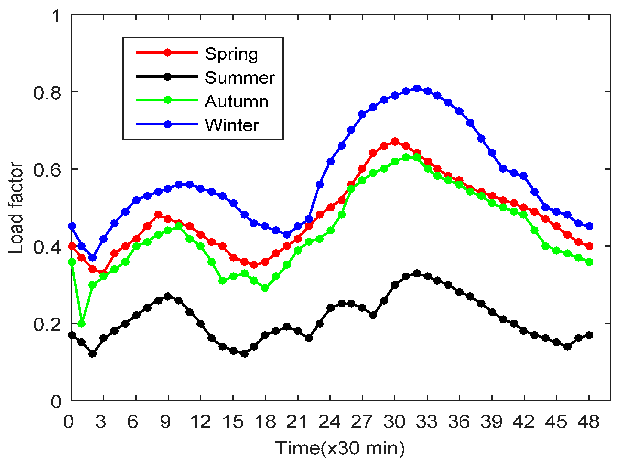
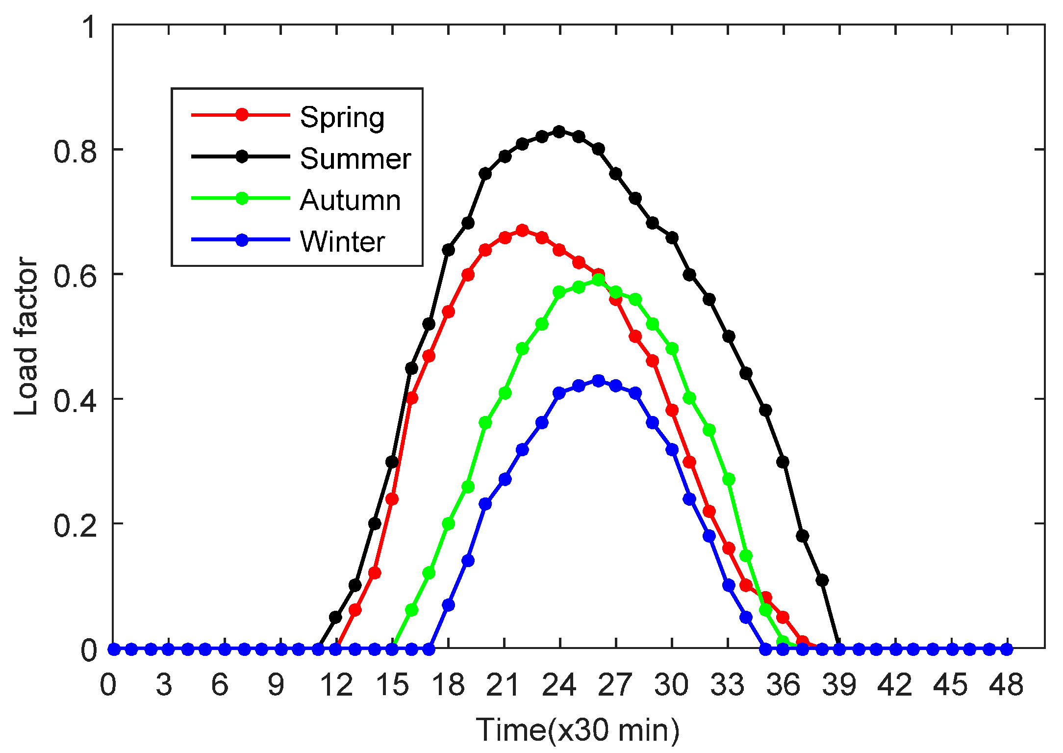
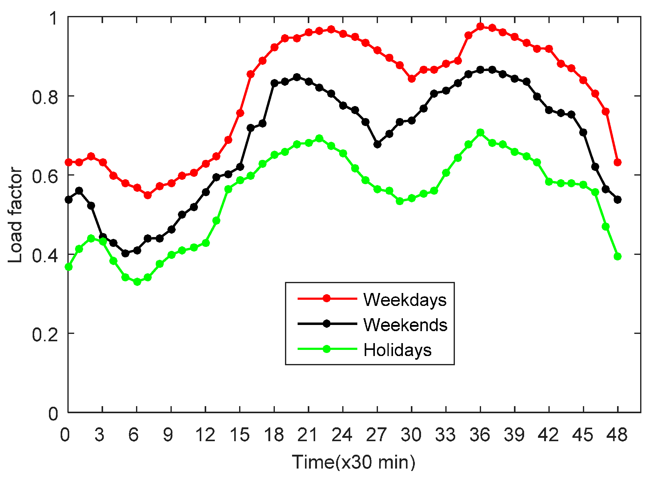
2.1. Analysis of the Timing Characteristics of the DG Output and Load Fluctuation

Taking into account the uncertainty of the DG output and load fluctuation, the model for each uncertain unit can be obtained. The wind power output mainly depends on the wind speed, and the change in wind speed is affected by natural environmental factors. Assuming that the probability model of the wind speed obeys the two-parameter (Weibull) distribution [50], and the probability distribution function is as follows:
F ( v ) = 1 exp [ ( v / c ) k ]
where v is the wind speed at the hub of fan impeller and k and c represent the shape parameter and the scale parameter, respectively.
The relationship between the fan output and wind speed can be approximated by the following piecewise function:
P W T G = { 0 0 v v i n c , v v o u t c P W T r v v i n c v r a t e d v i n c v i n c < v < v r a t e d P W T r v r a t e d < v < v o u t c
where PWTG and PWTr are the output power and the rated capacity of the fan, respectively, and vcin, vrated and vcout represent the cut in wind speed, the rated wind speed and the cut out wind speed, respectively.
The photovoltaic output is mainly affected by the illumination intensity, which depends on the seasonal variation and the changing weather. The illumination intensity usually obeys beta distribution [51], and its probability density function is as follows:
f ( I ) = Γ ( α + β ) Γ ( α ) Γ ( β ) ( I I max ) α 1 ( 1 I I max ) β 1
where I is the actual illumination intensity, Imax represents the maximum illumination intensity, α and β represent the shape parameters of the beta distribution, and Γ is the gamma function.
The relationship between the photovoltaic output and illumination intensity can be approximated by the following piecewise function:
P P V G = { P P V r I I max I I max P P V r I > I max
where PPVG and PPVr are the output power and the rated capacity of the photovoltaic, respectively.
The load fluctuation is easily affected by meteorological factors including the temperature, sunlight, humidity, rainfall, wind speed and wind direction, and these meteorological factors show different change patterns with the changing season. Additionally, the load fluctuation shows different trends with different days such as weekdays, Saturdays and holidays. Assuming that the load obeys a normal distribution [50], its probability density function is as follows:
f ( P L ) = 1 2 π σ L exp ( ( P L μ L ) 2 2 σ L 2 )
where PL is the actual load, μL represents the expected value of the load, and σL is the standard deviation of the load.
Based on the above model for each uncertain unit, on the annual sequence section, the wind power and photovoltaic output can be divided into four typical timing situations according to the differences among the seasons. For the load fluctuation, three types of dates are further classified for each season, and 12 typical timing situations can be obtained. To obtain four typical day curves of the wind power, photovoltaic output and load fluctuation based on a large amount of historical data on the wind power, photovoltaic output and load, a functional nonparametric regression model has been introduced in a previous study [52].
The wind power, photovoltaic output and daily load fluctuation of the electric power system essentially have functional characteristics, and the recorded daily load curves of these factors are functional types of data. The observed values from time t = 0 to t = nT are a continuous time series {Z(t), t € [0,nT]}. Based on the theory of functional data analysis, it can be transformed into a discrete functional time series {S1, S2, …, Sn}, and among them, Si = {Si(t1), Si(t2), …, Si(tp)}.
If one lets {(Xi, Yi), i = 1, 2, …, n} be the data pairs on the space FxR, then the functional regression model is established by (Xi, Yi), which is as follows:
Y i = r ( X i ) + ε i , i = 1 , 2 , , n
where the explanatory variable Xi is a function-type variable, the response variable Yi represents a real variable, the unknown function r is a regression function or a conditional mean function, and the error term εi is real random variable, which meets the condition E(εi|Xi) = (οi), and among them, E(˖) represents the expectation.
The key problem for the functional regression model is to estimate the regression function r by the known data. Therefore, based on the nonparametric kernel density estimation technique, the Nadaraya-Waston (N-W) kernel estimation method is used to estimate the functional type regression parameter r, and its estimation equation of the regression function is as follows:
r Λ ( x ) = i = 1 n K ( h 1 D ( x , X i ) ) Y i i = 1 n K ( h 1 D ( x , X i ) )
where K(˖) represents the kernel function that chooses the Gauss kernel function, h is the bandwidth that represents the effect of the kernel function near the sample point, and D(˖) is a semi metric that measures the degree of approximation between 2 function-type samples.

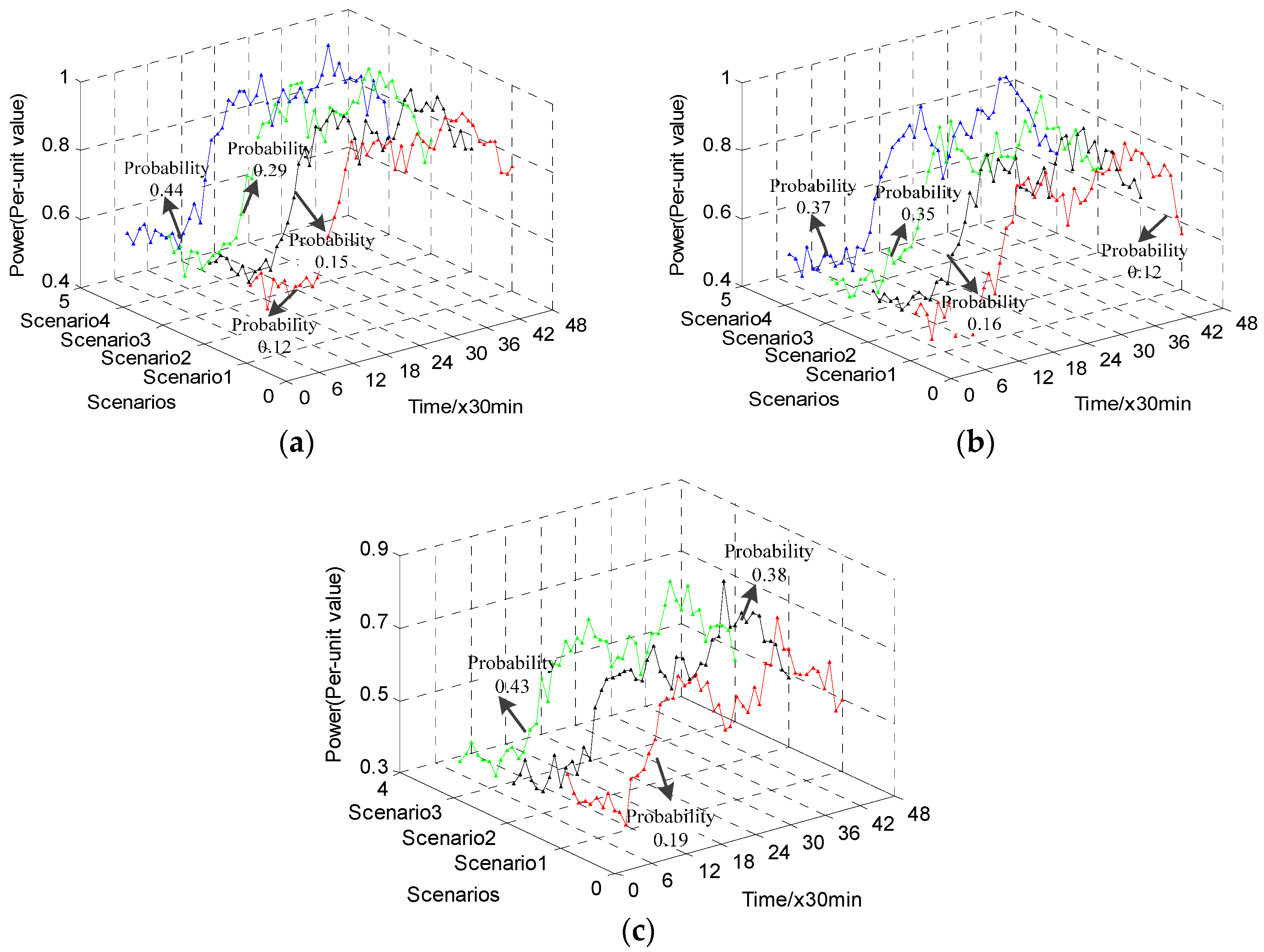
2.2. Multi-Scenario Construction Based on Time-Phasing and Hybrid Clustering

With the typical timing characteristics, although the typical daily curve can reflect the changing trend and a range of uncertainty, the fluctuation of each uncertainty unit is inevitably reduced. Therefore, based on the time-phasing of the DG output and load fluctuation, the improved FCM clustering algorithm is introduced. The clustering centres are obtained by clustering a large number of historical data, and the number of the clustering centres is the number of multi-scenarios constructed by the wind power, photovoltaic output and load fluctuation. Moreover, its probability indicates the occurrence possibility of the scenario.
For the traditional FCM clustering algorithm [53], in the absence of a class label given in advance, the largest degree of membership sample will be divided into one category through the iterative mode based on the objective functions. There is a certain blindness due to the human-made initial cluster centre and the total number of clusters. Therefore, the fast hill-climbing function method is introduced to determine the initial clustering centre and the number of clusters, which overcomes the subjectivity of the class number, avoids traps into the local minimum values and obtains an improved FCM clustering algorithm. The clustering process is as follows:
(1)
Initialize the degree of membership matrix U, introduce the fast climbing function method [54], and determine the number of initial clustering c and the initial clustering centre vi;
  • Define the pan type of the hill-climbing function:
    M ( v i ) = j = 1 n e α | | x j v i | | 2
    where α is a positive number that represents the effect for value M that is decided by the distance form of vi. The larger the value is, the more concentrated the data is, the finer the classification is, and the larger the M value is. Therefore, the clustering centre can be selected with a larger M value.
  • Select the sample sequentially, determine the tth hill-climbing function, and obtain the maximum value of each hill-climbing function M Λ t max and its corresponding load sample value x2*:
    M Λ t ( x p ) = M Λ t 1 ( x p ) M Λ t 1 max j = 1 n e β | | x j v i 1 | | 2
    where M Λ t ( x p ) is the tth hill-climbing function. M Λ t 1 ( x p ) and M Λ t 1 max are the t − 1th hill-climbing function and its maximum value, respectively.
  • Repeat step b until satisfying the convergence condition M Λ t max / M Λ 1 max δ , where δ is the convergence coefficient of the classification, which is a small positive number. The clustering number c is the total number of clustering iterations before the convergence is finished, and the initial clustering centre vi is the maximum sample value xt* of the hill-climbing function in each clustering process.
(2)
Determine the weighting index w, which determines the fuzzy degree of the final clustering effect as follows:
w * = { w | w ( J w ( U , V ) w ) = 0 }
where Jw(U,V) represents the objective function; that is, the distance weighted sum of squares of each sample to all clustering centres is defined as
J w ( U , V ) = j = 1 n i = 1 c u i j w | | x j v i | | 2
where vi is the ith vector of the clustering centre and uij is the degree of membership of the jth sample for the ith clustering centre.
(3)
Update the clustering centre and the degree of membership matrix as follows:
{ v i = j = 1 n u i j w x j j = 1 n u i j w ; 1 i c u i j = [ k = 1 c ( | | x j v i | | | | x j v k | | ) 2 w 1 ] 1 ; 1 i c , 1 j n
where xi (i = 1, 2, 3, …, c) is the set of ith load classification.
(4)
Use Equation (9) to calculate the objective functions.
(5)
Determine whether the iteration error of the two iterations of the objective function ∆Jw(U,V) is less than the given positive number ε, and if it is not satisfied, return to step 3. Otherwise, the clustering process ends.
In the typical timing situation based on the time-phasing, the clustering centres obtained by clustering a large number of historical data are the multi-scenario under this typical timing situation. Assuming that the number of the obtained clustering centres is k and the number of the objects contained in each cluster is n1, n2, …, ns, …, nk, the probability of the sth scenario is as follows:
p s = n s / i = 1 k n k
For a typical timing situation l, if the number of scenarios for the wind power, photovoltaic output and load are N W T l , N P V l , and N L l , respectively, the total number of scenarios in the typical timing situation is Nl = N W T l N P V l N L l . Similarly, the construction of the multi-scenario with timing characteristics can be obtained.

3. The Power Flow Calculation of the AC/DC Hybrid Distribution Network with VSC-MTDC

The current AC/DC hybrid DN is mostly based on voltage source converter-multi terminal direct current (VSC-MTDC) technology, and there may be multiple AC and DC regional areas that contain one or more branches. Therefore, the power flow calculation of the AC/DC hybrid DN based on VSC-MTDC technology by using the improved forward backward sweep power flow calculation method is introduced.

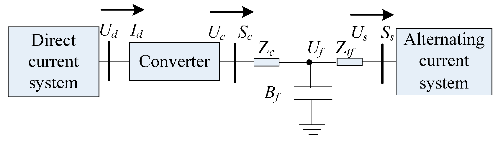
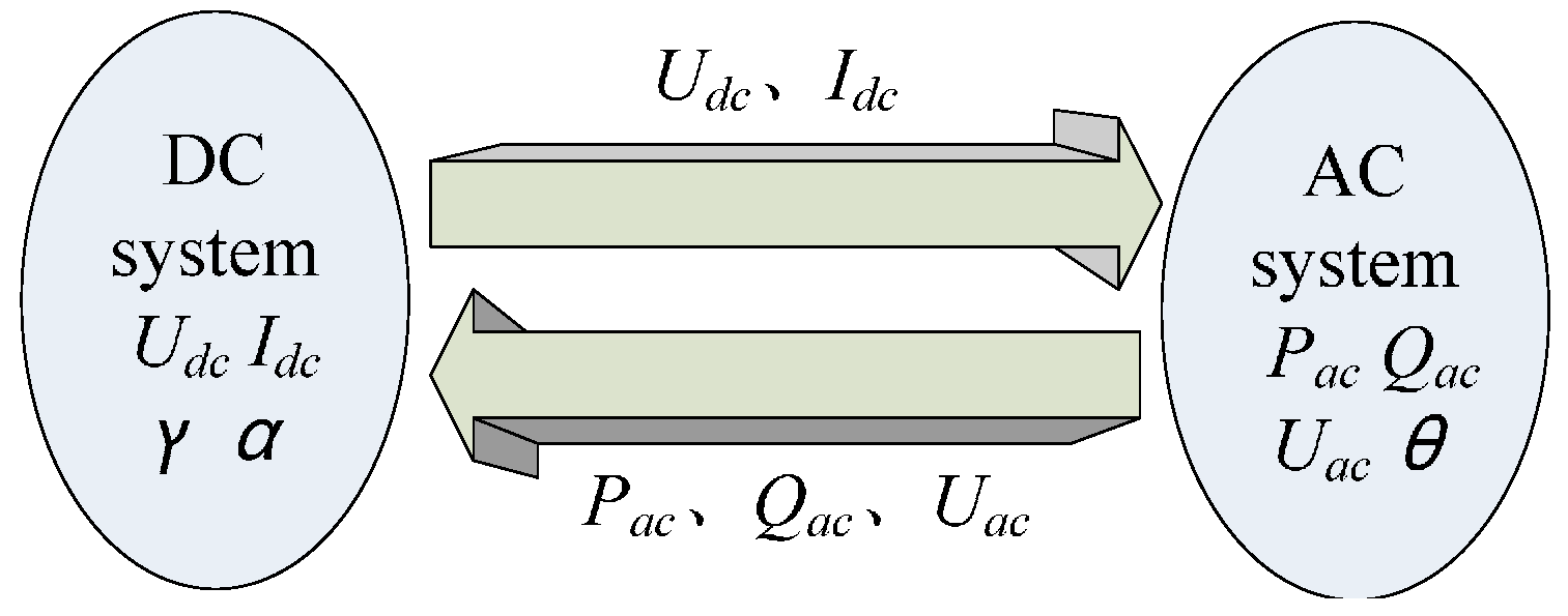
3.1. The Power Flow Calculation with VSC-MTDC

For the AC/DC hybrid DN with VSC-MTDC, the steady state model [55] of VSC-MTDC is shown in Figure 1.
In Figure 1, Ud and Id are the terminal voltage and the outflow current of the DC system, respectively. Setting the outflow active power of the DC system to Pd through the converter, the output voltage of the voltage source converter (VSC) is Uc < θc, the power is Sc = Pc + jQc, the outflow current is Ic, the reactor impedance is Zc = Rc + jXc, the converter transformer impedance is Ztf = Rtf + jXtf, the filter susceptance is Bf, the voltage at the filter is Uf < θf, the inflow power of the AC system is Ss = Ps + jQs, the voltage is Us < θs, and the phase-shifting angle of VSC is δ = θcθs.
The output power of the DC system from the converter and the input power of AC system are as follows:
{ P c = U c 2 G c U f t U c [ G c cos ( θ f θ c ) B c sin ( θ f θ c ) ] Q c = U c 2 B c + U f t U c [ G c sin ( θ f θ c ) + B c cos ( θ f θ c ) ] P s = U s 2 G t f + U s U f [ G t f cos ( θ s θ f ) + B t f sin ( θ s θ f ) ] Q s = U s 2 B t f + U s U f [ G t f sin ( θ s θ f ) B t f cos ( θ s θ f ) ]
The inverter often has a certain loss, which is related to the current Ic, and the loss consists of the following three parts: the constant, the primary function and the quadratic function:
P c o n v l o s s = a + b I c + c I c 2
where a, b and c are the corresponding loss coefficients, respectively.
The output voltage Uc of the converter is related to the terminal voltage Ud of the DC system, the modulation degree M and the DC voltage utilization factor μ, as follows:
U c = U d μ M 2
Thus, the power flow calculation with VSC-MTDC is determined.

3.2. The Power Flow Calculation of the AC/DC Hybrid Distribution Network with VSC-MTDC Based on Improved Forward-Backward Sweep

The power flow calculation based on forward-backward sweep [56] is calculated from the end of the system network to push forward in the AC/DC hybrid DN. In the process, the AC system and the DC system are alternately solved according to the topological structure, and then, the process is iterated until the result is converged. Thus, the power flow calculation of the AC/DC hybrid DN is completed. The alternating solution process is shown in Figure 2.
In Figure 2, Udc and Idc are the voltage and current value of the DC network, respectively; α and γ are the triggering angle and commutation overlap angle of the DC network, respectively; Pac, Qac, and Uac are the active power, reactive power and voltage value of the AC network, respectively, and θ is the phase-shifting angle of the AC network.
For the traditional power flow calculation based on a forward backward sweep, the calculation principle is simple, but the calculation period is long, and this method takes up a lot of storage space, which is not suitable for the power flow calculation of the complex DN. Therefore, we adopt the power flow calculation based on an improved forward-backward sweep method [57] and thus can determine the hierarchical division of the DN by optimizing the branches, nodes and branch numbers. The power flow calculation based on the improved forward-backward sweep method can use the branch-line parameters to calculate directly without the formation of an admittance matrix and triangular matrix. Thus, the voltage and power distribution can be calculated simply by algebraic equations, and a one-dimensional array is used to store the data, which may save a lot of storage space. Moreover, it improves the disadvantages that the power forward calculation and the voltage backward calculation cannot be calculated simultaneously and determines the parallel calculation of the power and voltage in the same level, which can further improve the calculation speed and shorten the calculation period of the power flow calculation.
For the power flow calculation based on the improved forward-backward sweep in the AC/DC hybrid DN, the calculation process is as follows:
(1) The hierarchical division principle of the AC/DC hybrid DN
The radiation type structure of the DN usually consists of a main feeder with several branches, and each branch has its own sub-branch. Therefore, regarding the power bus or the substation bus as the root node number, a main feeder is selected as the first layer, and the branches off the main feeder are encoded from the root node to the end node. Then, the branches under the same node of the main feeder are classified into the same hierarchy, and so on. As shown in Figure 3, the DN can be divided into eight levels, and the parallel computation of voltage and power can be divided into different branches within the same level.
(2) The power flow calculation based on the improved forward backward sweep at the same level
A. Calculate the forward power
For a multi-node network, when calculating the forward power and assuming that all unknown node voltages are the rated voltage of the grid, the power distribution of each branch can be calculated according to the load power, the system branch parameters and the power calculation sequence matrix as follows:
{ Δ S i j ( k ) = ( P j + P s u m , j ( k ) ) 2 + ( Q j + Q s u m , j ( k ) ) 2 V j ( k ) 2 ( r i j + j x i j ) S i j ( k ) = S s u m , j ( k ) + S j ( k ) + Δ S i j ( k )
where k represents the number of iterations; ∆Sij is the power loss of the branch corresponding to node i and j; Sij is the power of node i flowing to node j; Sj, Pj, and Qj represent the load power, active power and reactive power of node j, respectively; Ssum,j, Psum,j, and Qsum,j represent the sum of the load power, active power and reactive power of all branches with node j, respectively, that is, the head-end node; rij and xij are the resistance and reactance value of the branch corresponding to node i and j; and Vj is the voltage value of node j.
B. Calculate the backward voltage
The voltage of each node is calculated by using the sequential matrix that is calculated by the known head-end node voltage, the calculated power distribution and the voltage. Considering the large ratio of resistance to reactance (R/X) in the DN, the lateral component of the voltage drop cannot be omitted to improve the calculation accuracy. The voltage is calculated as follows:
{ Δ V j ( k + 1 ) = P i ( k ) r i j + Q i ( k ) x i j V i ( k + 1 ) δ V j ( k + 1 ) = P i ( k ) x i j Q i ( k ) r i j V i ( k + 1 ) V j ( k + 1 ) = ( V i ( k + 1 ) Δ V j ( k + 1 ) ) 2 + ( δ V j ( k + 1 ) ) 2
where ∆Vj and δVj are the longitudinal and lateral components of the voltage drop, respectively, and Pi and Qi are the active and reactive power of node i flowing to node j, respectively.
C. Determine whether the maximum value of the calculated amplitude difference for each node of the adjacent two iterations satisfies the given allowable error ε as follows:
max { | V i ( k + 1 ) V i ( k ) | } < ε
If ε is not satisfied, the next iteration is performed, and if it is satisfied, the voltage value of the last iteration is the output, and the iteration process is complete. In the AC/DC hybrid DN planning research, the VSC adopts the fixed Ud and Qs control mode when the AC system transforms to the DC system. When the DC system is converted to the AC system, the VSC adopts the fixed Us and θs control mode. In the power flow calculation, the VSC interface equation [58] of the AC/DC connection should be considered to obtain the equivalent injection power of the AC system. Taking the constant AC voltage control mode as an example, Us and θs are known. In the connected AC network, the node connected with VSC is regarded as the equilibrium node, and the power flow calculation based on the forward-backward sweep is calculated to obtain the injection power Ps and Qs of the AC system. Then, the following calculations are performed:
{ U f = U s + ( S s / U s ) * Z t f S c f = U f ( S s / U s ) + j ( B f U f 2 ) I c = ( S c f / U f ) * U c = U f + I c Z c P c + j Q c = S c = U c I c * P d = P c + ( a + b I c + c I c 2 )
At this time, the phase-shifting angle δ can be obtained according to Us and Uc, the power flow calculation of the DC DN can be continued, and Ud can be calculated when Pd is known. In addition, according to Equation (16), the modulation degree M can be obtained. Then, the power flow calculation based on the forward-backward sweep of the AC/DC hybrid DN with VSC-MTDC is determined.

4. The Multi-Objective Coordinated Planning of the AC/DC Hybrid Distribution Network Based on the Multi-Scenario Technique Considering Timing Characteristics

In the multi-objective planning of the AC/DC hybrid DN, planning of the DG configuration includes the following: the installation locations, the types and capacity of the DG, and the planning of network frames referring to the transformation of the AC lines into DC lines, the access location of the DC line for building the DC network and whether the building line is the DC line.

4.1. Objective Functions

(1) The Minimum Annual Economic Cost is as follows:
min f 1 = C D G i o m + C l i n e + C D G c o n v + C l o a d c o n v + C l i n e c o n v
where C D G i o m , Cline, C D G c o n v , C l o a d c o n v and C l i n e c o n v are the costs of DG investment, operation and maintenance; the costs of transforming some of the AC lines into DC lines and building the DC network; the costs of the DG connected to the converter; the costs of the connected converter for load; and the costs of the converter on the DC line system. Among them, the cost of the AC/DC or DC/AC converter required by the increase in the DC load is reflected in C l o a d c o n v , while the cost of the converter needed for the connection between the DC subsystem and the AC system is reflected in C l i n e c o n v :
C D G i o m = i = 1 N D G α g , i g = 1 G D G C g S i , g λ g + i = 1 N D G j = 1 N t d j s = 1 N s , j p s , j t = 1 T Δ t g = 1 G D G C g , o m P g , i j s t
where NDG represents the total number of DG candidate nodes; αg,i is the fixed annual average cost factor for the installation of DG for node i; GDG is the type number of DG; Nt represents the total number of typical timing situations for the DG output and load fluctuation; dj is the number of dates of the typical timing situation j in a year; Ns,j represents the number of scenarios under a typical timing situation j; ps,j represents the occurrence probability of scenario s under a typical timing situation j; T is the number of time intervals in the day; ∆t is the unit of time duration; Cg and λg represent the unit of active capacity investment cost and the power factor of the gth class DG, respectively; Si,g is the rated capacity of the gth class DG installed at the candidate node i; Cg,om is the unit power generation capacity operation and maintenance costs of the gth class DG; Pg,ijst represents the active output of the gth class DG installed at the candidate node i in the period t of the scenario s under the typical timing situation j:
C l i n e = i = 1 N u p α l , i x i l i C l d c + j = 1 N n e w α l , j ( x j a c l j a c C l a c + x j d c l j d c C l d c )
where Nup is the total number of lines for the DC line reformed; Nnew is the total number of newly built lines; αl,i and αl,j represent the annual average cost coefficients for line i and line j, respectively; C l a c and C l d c are the unit length costs of the AC lines and DC lines, respectively; xi, x j a c , and x j d c represent 0–1 variables, which indicate the DC transformation line i and the AC or DC newly built line j, respectively; li, l j a c , and l j d c are the length of the DC transformation line i and the AC or DC newly built line j, respectively:
C D G c o n v = i = 1 N D G α c x i , g a c g = 1 G D G C c o n v S i , g λ g
where Cconv represents the unit active capacity cost of the converter; αc is the annual average cost coefficient of the converter; and x i g a c represents the 0–1 variable that indicates whether node i accessed by the DG is the AC node:
C l o a d c o n v = i = 1 N n o d e α c C c o n v P L , i ( x L , i a c η i a c + x L , i d c η i d c )
where Nnode represents the total load node; PL,i is the active load of node i; x L i a c , x l i d c represent the 0–1 variable, x L i a c indicates whether the load of the node i is connected to the DC/AC converter, and x l i d c indicates whether it is an AC/DC converter; and η i a c , η i d c represents the ratio of the AC load and DC load of node i, respectively:
C l o a d c o n v = i = 1 N n o d e α c C c o n v P L , i ( x L , i a c η i a c + x L , i d c η i d c )
where Pi,conv and Pj,conv represent the capacity of converter to be upgraded on the DC transformation line i and the AC or DC newly built line j, respectively.
(2) The Minimum Annual Network Loss is as follows:
min f 2 = j = 1 N t d j s = 1 N s , j p s , j t = 1 T Δ t ( P c o n v , j s t l o s s + i = 1 N b r P i , j s t l o s s )
where Nbr is the total number of system branches and P c o n v , j s t l o s s and P i , j s t l o s s are the loss of the converter in the system and the branch i within the period t under the typical timing situation j in the scenario s, respectively.
(3) The best stability of annual average voltage of the system is as follows:
L a b = j = 1 N t 1 N t s = 1 N s , j p s , j t = 1 T 1 T [ 4 ( P b , j s t X a b Q b , j s t R a b ) 2 + ( P b , j s t R a b + Q b , j s t X a b ) U a , j s t 2 U a , j s t 4 ]
{ min f 3 = min L V S L V S = max { L 1 , L 2 , , L N b r }
where Rab and Xab are the resistance and reactance of line ab, respectively; Ua,jst, Pb,jst, and Qb,jst represent the head-end node voltage of the line ab and the active and reactive power flow at the end of the line within the period t under the typical timing situation j in the scenario s, respectively. Among them, Equation (28) is the expected value of the voltage stability index based on the multi-scenario with timing characteristics for the single line ab, and the Equation (29) is the expected value of the annual average voltage stability index of the system. The voltage stability index can reflect the voltage stability of each branch for the DN, and the smaller the index is, the better the voltage stability is.

4.2. Constraint Conditions
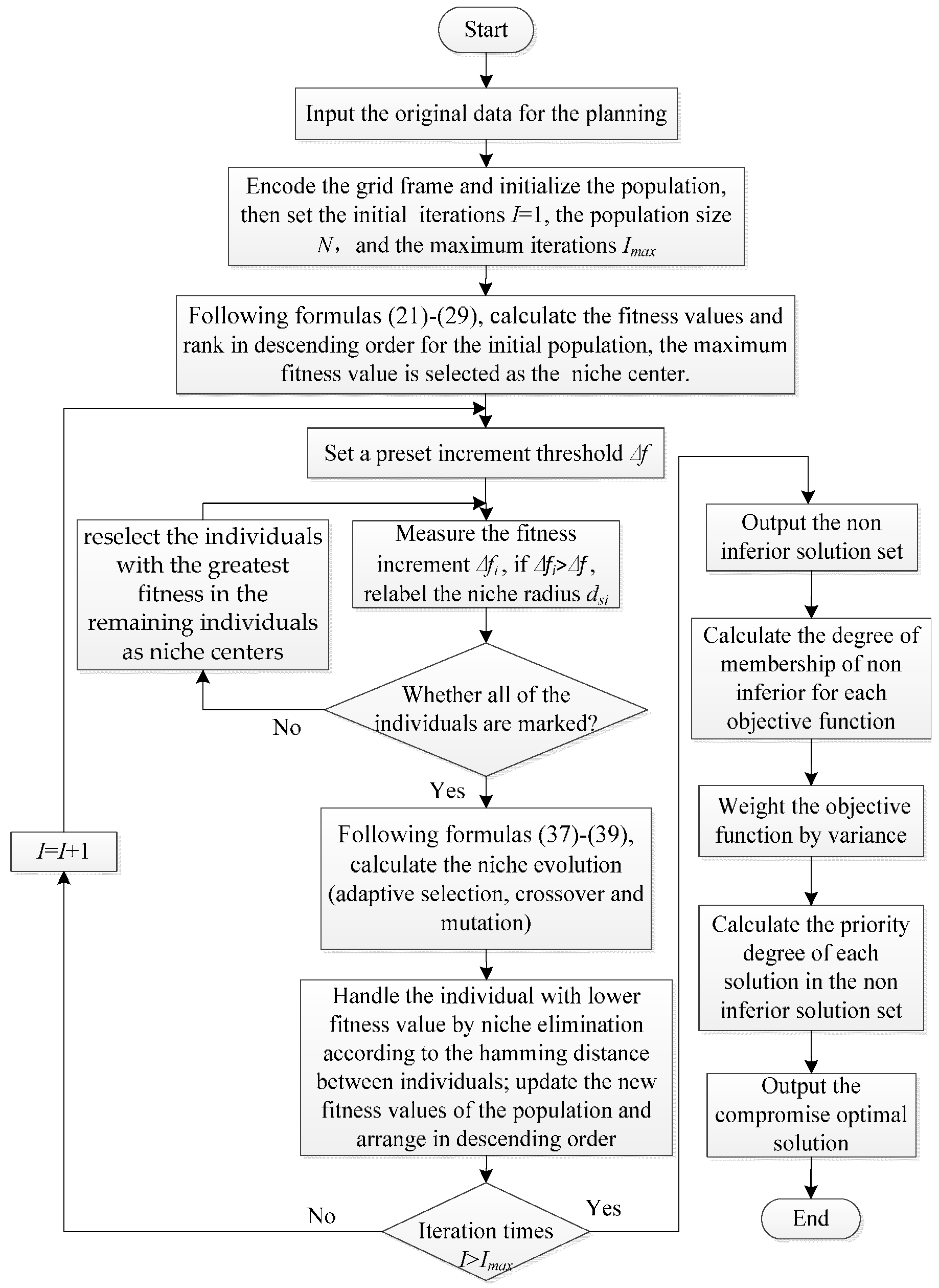
The constraint conditions include the power balance constraint of the AC node, the power balance constraint of the DC node, the upper and lower bound constraints of the node voltage, the branch power limit constraint, and the DG capacity constraint:
{ P i a c = U i a c j = 1 N n o d e U j a c ( G i j cos θ i j + B i j sin θ i j ) Q i a c = U i a c j = 1 N n o d e U j a c ( G i j sin θ i j B i j cos θ i j )
{ ± I i d c j = 1 N d c g i j U j d c = 0 P i d c = I i d c U i d c
U i min U i U i max
P i j P i j max
{ 0 S i , g λ g P i , g max g = 1 G D G S i , g λ g P i , max i = 1 N D G g = 1 G D G S i , g λ g σ g P L
where P i a c and Q i a c are the active and reactive injection power of the AC node i, respectively; Gi and Bij represent the conductance and susceptance of branch ij, respectively; θij is the voltage phase difference between node i and node j; Ndc is the set of DC nodes; gij represents the conductance of branch ij; I i d c , U i d c , and P i d c are the current, voltage and power of the DC node i, respectively; U j d c is the voltage of the DC node j; U i max and U i min represent the upper and lower voltage of node i, respectively; Pij and P i j max represent the active power and the upper limit power of branch ij, respectively; P i , g max and Pi,max are the maximum active capacity of the gth class DG that is node i allowed to access and the maximum capacity of all the types DG; σg is the maximum active capacity penetration rate of DG; and PL represents the total active load of the system.

4.3. Model Solution

To solve the multi-objective coordinated planning model of the AC/DC hybrid DN based on multi-scenario with timing characteristics, an improved adaptive niche genetic algorithm based on fuzzy degree of membership and variance weighting is used to solve the nested model. The particle is coded in a binary structure, which is as follows:
C c o d e = { T 1 S 1 , T 2 S s , , T N D G S N D G , U 1 , U 2 , , U N u p , N 1 D 1 , N 2 D 2 , , N l D l }
where Ti and Si represent the grid DG type and grid DG capacity on the DG candidate position i, respectively; Ui represents whether the DC is to be reformed in the ith pending a reformation line; Ni and Di denote the number of the access line of the amplification load point i and whether it is a DC line, respectively; and l is the number of new load points.
To improve the adaptive niche genetic algorithm [59], to maintain the diversity of the population and obtain a better global search performance, the adaptive genetic algorithm and the sigmoid function combined with cosine transform are introduced. Then, the crossover rate pc and the mutation rate pm can be obtained according to the individual fitness value of the population, and the method of fuzzy degree of membership and variance weighting [60] is used to calculate the priority of each particle in the non-dominated solution set after the iteration. The particle with the highest priority is the final compromise optimal solution. The model solution is as follows:
(1)
Input the original data for the planning, encode the grid frame and initialize the population, randomly generate N populations and calculate the fitness values and rank in descending order according to Equations (21)–(29). Take the individual with the greatest fitness as the first centre of the niche, marked as Sc.
(2)
Measure the fitness increment Δfi of each individual and compare it with a pre-set increment threshold Δf. If the fitness rate exceeds the threshold, the distance from the individual to Sci can be used as the niche radius dci. The Δfi is as follows:
Δ f i = f ( s c i + 1 ) f ( s c i ) f max f min
(3)
For other unlabelled individuals, reselect the individuals with the greatest fitness from the remaining individuals as niche centres, and repeat processes (1) and (2) until all individuals are marked.
(4)
The adaptive selection, crossover and mutation by means of Equations (37) and (38) are used to calculate the fitness value of the new generation population, and then, the average fitness value of each niche population is calculated according to Equation (39).
p c = { p c 2 + p c 1 2 + p c 2 p c 1 2 cos [ 2 π 1 + exp ( β f f a v g f max f a v g ) ] , f f a v g p c 1 , f f a v g
p m = { p m 2 + p m 1 2 + p m 2 p m 1 2 cos [ 2 π 1 + exp ( β f f a v g f max f a v g ) ] , f f a v g p m 1 , f f a v g
f a v g = k = 1 n f k / n
where α and β are the constant parameters; pc1 and pc2 represent the minimum and maximum of the crossover rate, respectively; pm1 and pm2 represent the minimum and maximum values of the variance, respectively; fmax is the largest fitness value of the population; favg is the average fitness of each population; f′ is the larger fitness value of the two individuals to be crossed; and f is the individual fitness value to be mutated.
(5)
Use the penalty function of Equations (30)–(34) and handle the individuals with a lower fitness value by niche elimination. According to the hamming distance between the individuals, update the new fitness values of the population and arrange them in descending order;
(6)
Determine whether the number of iterations reaches the upper limit, if it is not satisfied, return to step (2), and if it is satisfied, then the iteration process is finished, and the non-inferior solution set will be output.
(7)
Calculate the degree of membership of non-inferior for each objective function according to Equation (40) as follows:
ε i j = g j max g i j g j max g j min , j = 1 , 2 , 3
where gij is the jth objective values of the ith solution in the non-inferior solution set and g j max and g j min are the maximum and minimum values of the objective j, respectively.
(8)
Weight the objective function by variance according to Equation (41) as follows:
w j = i = 1 N k = i N ( ε i j ε k j ) 2 l = 1 M i = 1 N k = i N ( ε i l ε k l ) 2
where wj is the weight of the objective j, M is the number of the objective function, and N is the number of the non-inferior solution set.
(9)
According to Equation (42), calculate the priority degree of each solution in the non-inferior solution set, and output the particle with the greatest degree that is the compromised optimal solution as follows:
S i = j = 1 M ε i j w j
The flow chart of the improved adaptive niche genetic algorithm based on the fuzzy degree of membership and variance weighting is shown in Figure 4.

5. Example Analysis

5.1. The Construction and Analysis of a Multi-Scenario

Due to the obvious seasonal variations in wind power and photovoltaic power, combined with a large amount of historical data, the typical timing characteristic curves of wind power, photovoltaic power and load fluctuation can be obtained by the functional nonparametric regression models in Section 2.1, which are shown in Figure 5 and Figure 6.
As seen from Figure 5 and Figure 6, the trends of wind power output and PV output are similar and are lower than the rated load values in different seasons. However, the wind power output and PV output at the same moment in different seasons are obviously distinct, which further characterizes the uncertainty of the wind power and photovoltaic output. The wind power output each season from greatest to least decreases in accordance with the order is winter, spring, autumn and summer, which indicates the characteristics that the wind speed is large in winter and small in summer. The PV power output from greatest to least each season is summer, spring, autumn and winter which is closely related to the high illumination intensity in summer and the low illumination intensity in winter.
The load fluctuation is not only related to the seasonal differences but also closely related to the dates. Therefore, with a minimum time scale of 30 minutes of load history data, taking the spring as an example, the typical timing characteristic curves of load fluctuation are obtained as shown in Figure 7. As seen from Figure 7, the typical timing characteristic curves of load fluctuation with different dates have differing variation ranges, and the load values have obvious differences at the same moment. The load fluctuation from greatest to least is weekdays, weekends and holidays, which is due to the large, industrial and commercial electrical demand.
During the holidays, many people choose to go out of the home to play, and thus, the load value significantly decreases on holidays. These fluctuations are closely related to people’s working conditions, electricity habits, power consumption time and other factors, which also characterize the uncertainty of load fluctuation. Although the typical timing characteristic curves of wind power, photovoltaic power and load fluctuation can roughly reflect the scope and trend of the uncertainty, they also inevitably reduce the fluctuation of each uncertainty unit. Taking PV as an example, the actual PV output is not only affected by seasonal factors but also closely related to the type of weather. In addition, judging and extracting the specific types of weather from a large number of historical data is not easy, and analysing the typical daily curve of the extreme weather is not feasible. Therefore, an improved FCM clustering algorithm is used to simulate a four-season scenario figure of wind power, photovoltaic output and load fluctuation with the consideration of the data type differences. Through the analysis of the multi-scenario technology, the uncertainty of each unit is enhanced. The scenarios of wind power output and photovoltaic power output for the four seasons are shown in Figure 8 and Figure 9.
For the load fluctuation, using the spring scenario as an example, the load fluctuations on weekdays, weekends and holidays are shown in Figure 10.
From Figure 8, Figure 9 and Figure 10, we can conclude the following: For each typical timing characteristic curve of wind power, photovoltaic output and load fluctuation, the clustering algorithm can be used to construct the multi-scenario; the different multi-scenario curves are several discrete scenes with small differences in the typical situations; and their probabilities indicate the possibility of the scenario occurring. Compared with the single typical daily curve, the coverage area of the multi-scenario curve is larger, the volatility is enhanced, and it better estimates the extreme situations. Therefore, the uncertainty of the DG output and load fluctuation is further characterized.
Based on the seasonal differences, the number of scenarios with the typical timing characteristics of wind power and photovoltaic output include 4, 3, 4, and 5 and 5, 4, 5, and 4. Based on the seasonal and date differences, the numbers of scenarios with the typical timing characteristics of load fluctuation are 4, 4, 3, 4, 3, 3, 4, 4, 3, 4, 4, and 3. Therefore, in the annual timing sequential, there will be 780 scenarios with the three kinds of uncertain elements that are aggregated in the typical timing characteristics. The number of scenarios in the typical timing characteristics is shown in Table 1.

5.2. The Planning of the AC/DC Hybrid Distribution Network Based on Multi-Scenario Technique Consideration Timing Characteristics

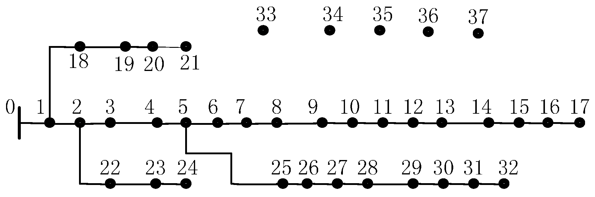
5.2.1. The Overview Example and Parameter Analysis

Based on the construction and model analysis of the multi-scenario with timing characteristics and taking the IEEE33 node power distribution system as an example, the topological structure is shown in Figure 11.
In the topological structure of the IEEE33 node power distribution system, the node 0, which can be regarded as the power point of the system, is the balance node, and the other nodes are the load nodes. The initial system contains 33 nodes and 32 branches. The rated voltage is 12.66 kV, and the overall load is 3715 kW + j2300 kvar. With a greater DC load increase, each load node in the system will no longer be a simple AC load node. To adapt the reconstruction planning of the AC/DC hybrid DN, some reformation in the system will be made. On the basis of the original total load, the proportions of the AC and DC loads for each node of the system are reset, which shown in Table 2.
Additionally, on the basis of the original system, a five-load node will be amplified, including nodes 33, 34, 35, 36 and 37. The total increased load is 600 kW + j320 kvar, and the proportions of the DC load of each of the new load nodes are 0%, 30%, 50%, 70% and 100%, respectively. Each load node that is connected to the system can connect with one of the 32 nodes besides the balance node, but only one line that can be built by the DC or AC node is allowed access. For the DC line transformation, all the existing lines in the system can be used as the candidate lines to optimize the planning decision-making.
The construction cost of the AC line is 7 × 10⁴ yuan/km, and the construction cost of the DC line is 2 × 10⁴ yuan/km. In the AC DN, the photovoltaic power supply is DC power, which is grid-connected by the DC/AC converter. The wind power can generate both the DC power and the AC power, which is grid-connected by the DC/AC or AC/DC/AC converter. Therefore, the converter link will be omitted if two types of DG are directly incorporated into the DC subsystem. For the wind power, the installation cost is 6 × 10³ yuan/kW, and the operation and maintenance cost is 0.2 yuan/(kW·h). For the photovoltaic system, the installation cost is 8 × 10³ yuan/kW, and the operation and maintenance cost is 0.15 yuan /(kW·h). The average annual investment cost coefficient of the DG is 0.1, and the power factor is 0.85. Considering the proportion of the DC load in each load node, the candidate nodes for the DG are 7, 10, 12, 13, 14, 16, 17, 18, 19, 20, 22, 23, 24, 25, 26, 29, 30, 31, and 32. The minimum unit capacity of the grid-connected DG is 60 kVA, and if the grid-connected cardinal number is m (m = 0, 1, 2, …, 7) for a node in a certain type DG, the installation capacity of this node is m × 60 kVA.

5.2.2. The Planning Result Analysis

(1) Considering the Planning of Transforming Part of the AC Lines into DC Lines and Building the DC Network
For the planning variables, considering transforming part of the AC lines into DC lines and building the DC network, the DG configuration, the DC line transformation results and the newly built line configuration can be obtained from the model as shown in Table 3.
The structure of the AC/DC hybrid DN after the planning is shown in Figure 12. In Figure 12, the red lines represent the DC transformation lines, the blue lines represent the newly built DC lines, the purple lines represent the newly built AC lines, and the green lines represent the type and capacity of the DG installation in the nodes. The layout situation of the DC transformation lines, DG installation locations and newly built AC and DC lines can be seen more clearly in Figure 8.
Table 3 and Figure 12 show that the DC transformation lines are basically located around the nodes with a higher DC load density such as nodes 13, 17, 23, 30 and 31, and most of the DC lines are at the end of the system such as nodes 17, 24 and 31. Therefore, the DC transformation lines can reduce the converter capacity and investment cost. For the position of the grid-connected DG, the nodes are at one end of the DC line, except for nodes 7 and 20, and thus may decrease the converter link and reduce the loss of the investment cost. According to the DC load ratio of the new load node, the appropriate accessing network form of the new lines can be chosen, such as nodes 35, 36 and 37 with a higher proportion of the DC load. Thus, the corresponding newly built lines are constructed to the DC lines, and the end node of the DC subsystem is selected to insert them in the DN.
To coordinate grid connection between the photovoltaic power and wind power, the best matching property of the grid connected system can be obtained, and the acceptance degree of the wind power is larger than the photovoltaic power. This may be due to better matching of the wind power output and load fluctuation in the timing characteristics, and the daily output of the wind power is relatively higher in most cases. The objective function values after the planning are shown in Table 4. As shown in Table 4, in the AC/DC hybrid DN, most of the DG in the DC subsystem can save many costs due to the reduction of the converter link, and the DC load area with a high density also reduces the converter cost due to the formation of the DC subsystem.
(2) Without Considering the Planning of Transforming Part of the AC Lines into DC Lines and Building the DC Network
Without considering the planning of transforming part of the AC lines into DC lines and building the DC network, the planning results are shown in Table 5.
The structure of the AC DN after the planning is shown in Figure 13; the purple lines represent the newly built lines, and the green lines represent the type and capacity of the DG installation in the nodes.
Table 5 and Figure 13 together demonstrate that compared with considering DC line transformation and the newly built DC line, the grid-connected capacity of the DG has been greatly reduced. Among them, the grid-connected capacity of wind power decreases by 240 kVA, which accounts for 28.6% of all of the grid-connected wind power, and the grid-connected capacity of photovoltaic power decreases by 180 kVA, which accounts for 27.3% of all of the grid-connected photovoltaic power. Thus, due to the reduction of the converter link in the AC/DC hybrid DN, not only are the network loss and investment costs reduced, but also, the consumption of the DG is greater. The objective function values compared with the considered DC planning scheme are shown in Table 6.
Comparing with the DC line transformation and newly built DC line, the annual investment, operational and maintenance costs of the DG and the DC line transformation and the newly built DC line costs are reduced by 11.42 million yuan and 0.042 million yuan, respectively, which are not much different. However, the costs of converting the grid-connected DG and the costs of converting the connected load are increased, and the increased costs are 23.02 million yuan and 21.143 million yuan, respectively. That is because for the planning scheme without considering DC line transformation and a newly built DC line, the consumption of a large number of DC load is still in the AC DN. Although the DC line transformation costs are 0, the converter of grid-connected DG costs and the converter of load connected costs rise sharply. Thus, the final cost is higher than the planning scheme of considering DC line transformation and newly built DC line, and the cost increased by approximately 6.101 million yuan, which accounted for 3.32% of the total annual economic costs. Additionally, the annual active network loss is far lower than the AC DN, which is 339.33 MW·h, accounting for 27.74% of the total annual active network loss after the DC line transformation and newly built DC line of the AC/DC hybrid DN. Meanwhile, the voltage stability becomes better, and the annual average voltage stability index is reduced from 0.091 to 0.062.
Figure 14 shows a contrast chart of the annual average voltage stability index with whether there is a consideration of the DC line transformation and newly built DC line.
With the plan considering the DC line transformation and newly built DC line in the AC/DC hybrid DN, the branches 13, 17, 20, 23, 24, 30 and 31 are transformed into DC lines, and the branches 35, 36 and 37 are the newly built DC lines. For these DC branches, there will be no stability problems; thus, the index values are set to 0. Also shown in Figure 14 is that the annual average voltage stability index for each branch of the AC/DC hybrid DN is lower than that of the AC DN, and its voltage stability is similarly better.

6. Conclusions

In this paper, a functional nonparametric regression model is established, and the multi-scenario construction of the DG output and load fluctuation with timing characteristics is introduced. Then, the power flow calculation method based on an improved forward-backward sweep for the AC/DC hybrid DN with VSC-MTDC is described. With increased DC load density and penetration of a large number of DG units for the AC DN, considering the DC DN advantages of low network loss, good power quality and easy acceptance of the DG, a planning approach considering transforming some of the AC lines into DC lines and building a DC network is put forth. Based on this, a planning model for an AC/DC hybrid DN with DG based on the construction of multi-scenario technology with timing characteristics is built. Finally, through the example simulation, the construction of multi-scenario technology in typical timing characteristics is obtained, and the uncertainty of each DG and load fluctuation is described more accurately. In comparison to not planning to transform some of the AC lines into DC lines and build a DC network in the DN planning, more DG units can be admitted when planning to transform some of the AC lines into DC lines and build a DC network, and due to reducing the grid DG and the inversion link of load consumption, the overall cost of the AC/DC hybrid DN is reduced. Moreover, the power quality of the AC/DC hybrid DN is notably improved, and the active power network loss and voltage stability index are better than those of the planning model when considering the AC DN alone. Thus, the correctness and effectiveness of the proposed planning method are verified, and a certain amount of reference is provided for the future DN optimization planning and deeper research of the AC/DC hybrid DN. However, this paper only puts forward a preliminary assumption for the plan to transform some of the AC lines into DC lines and build a DC network. In the future, the bi-level coordinated planning model for the DG and network frame in the AC/DC hybrid DN should be considered. Thus, the optimization decision for the configuration of the network frame and the DG is carried out in the upper level and lower level, which can ensure the optimal combination of the DG and DN frame. Therefore, the mutual interaction of the DG and DN frame can be addressed. However, we can further consider the partition planning of the DN; namely, the plan to transform some of the AC lines into DC lines and build a DC network should be planned for the DN area with a higher DC load, and the centralized transformation can be carried out, which will be more conducive for the security, stability and economic development of the AC/DC hybrid DN.

Acknowledgments

The authors would like to acknowledge the National Natural Science Foundation of China (51607068) and the Beijing National Science Foundation (3164051).

Author Contributions

The author Xiaodan Wang carried out the main research tasks and wrote the full manuscript, Yongchun Yang and Yajing Gao analysed, proposed the original idea, double-checked the results and the whole manuscript, Jingjing Luo and Jie Duan contributed to writing and summarizing the proposed ideas and English translation integration. While Hong Li and Xiangning Xiao provided technical and financial support throughout.

Conflicts of Interest

The authors declare no conflict of interest.

Abbreviations

The following abbreviations are used in this manuscript:
DGDistributed generation
DNDistributed networks
ACAlternating current
DCDirect current
EVsElectric Vehicles
DSDistributed storage
ATCavailable transfer capability
HVDCHigh Voltage Direct Current
GATGeneral Analytical Technique
RDSsRadial Distribution Systems
SPPVSsSingle-Phase Photovoltaic Systems
PATProposed Analytical Technique
BFGEsBiomass-fueled gas engines
FCMFuzzy C means
VSC-MTDCVoltage source converter-multi terminal direct current

References

  1. Whaite, S.; Grainger, B.; Kwasinski, A. Power Quality in DC Power Distribution Systems and Microgrids. Energies 2015, 8, 4378–4399. [Google Scholar] [CrossRef]
  2. Gao, Y.; Yang, W.; Zhu, J.; Ren, J.; Li, P. Evaluating the Effect of Distributed Generation on Power Supply Capacity in Active Distribution System Based on Sensitivity Analysis. Energies 2017, 10, 1473. [Google Scholar] [CrossRef]
  3. Montoya-Bueno, S.; Muñoz-Hernández, J.I.; Contreras, J. Uncertainty management of renewable distributed generation. J. Clean. Prod. 2016, 138, 103–118. [Google Scholar] [CrossRef]
  4. Monadi, M.; Rouzbehi, K.; Candela, J.I.; Rodriguez, P. Chapter 11-DC Distribution Networks: A Solution for Integration of Distributed Generation Systems. In Distributed Generation Systems; Elsevier: Amsterdam, The Netherlands, 2017; pp. 509–561. ISBN 978-0-12-804208-3. [Google Scholar]
  5. Xue, S.; Lian, J.; Qi, J.; Fan, B. Pole-to-Ground Fault Analysis and Fast Protection Scheme for HVDC Based on Overhead Transmission Lines. Energies 2017, 10, 1059. [Google Scholar] [CrossRef]
  6. Jialiang, W.; Rui, W.; Chang, P.; Yu, W. Analysis of DC Grid Prospects in China. Proc. CSEE 2012, 32, 7–12. [Google Scholar]
  7. Hakala, T.; Lahdeaho, T.; Jarventausta, P. Low voltage DC distribution–utilization potential in a large distribution network company. IEEE Trans. Power Deliv. 2015, 30, 1694–1701. [Google Scholar] [CrossRef]
  8. Younus, S.A.M.; Nardello, M.; Tosato, P.; Brunelli, D. Power Controlling, Monitoring and Routing Center Enabled by a DC-Transformer. Energies 2017, 10, 403. [Google Scholar] [CrossRef]
  9. Hernandez, J.C.; Sanchez, F. Electric Vehicle Charging Stations Fed by Renewables: PV and Train Regenerative Braking. IEEE Lat. Am. Trans. 2016, 14, 3262–3269. [Google Scholar] [CrossRef]
  10. Liu, X.; Dai, X.; Li, M. Research on the home energy management system based on the microgrid technology. Power Syst. Prot. Control 2017, 45, 66–72. [Google Scholar]
  11. Diaz, N.L.; Dragičević, T.; Vasquez, J.C.; Guerrero, J.M. Intelligent distributed generation and storage units for dc microgrids—A new concept on cooperative control without communications beyond droop control. IEEE Trans. Smart Grid 2014, 5, 2476–2485. [Google Scholar] [CrossRef]
  12. Sun, K.; Zhang, L.; Xing, Y.; Guerrero, J.M. A distributed control strategy based on dc bus signaling for modular photovoltaic generation systems with battery energy storage. IEEE Trans. Power Electron. 2011, 26, 3032–3045. [Google Scholar] [CrossRef]
  13. Wang, P.; Jin, C.; Zhu, D.; Tang, Y.; Loh, P.C.; Choo, F.H. Distributed control for autonomous operation of a three-port AC/DC/DS hybrid microgrid. IEEE Trans. Ind. Electron. 2015, 62, 1279–1290. [Google Scholar] [CrossRef]
  14. Guo, L.; Zhang, S.; Li, X.; Feng, Y. Hierarchical coordination control for DC microgrid considering time of-use price. Power Syst. Technol. 2016, 40, 1992–2000. [Google Scholar]
  15. Lu, X.; Liu, N.; Chen, Q.; Zhang, J. Multi-objective optimal scheduling of a DC micro-grid consisted of PV system and EV charging station. In Proceedings of the 2014 IEEE Innovative Smart Grid Technologies, Asia, Kuala Lumpur, Malaysia, 20–23 May 2014; pp. 487–491. [Google Scholar]
  16. Shaaban, M.F.; Eajal, A.A.; El-Saadany, E.F. Coordinated charging of plug-in hybrid electric vehicles in smart hybrid AC/DC distribution systems. Renew. Energy 2015, 82, 92–99. [Google Scholar] [CrossRef]
  17. Sechilariu, M.; Locment, F.; Wang, B. Photovoltaic Electricity for Sustainable Building. Efficiency and Energy Cost Reduction for Isolated DC Microgrid. Energies 2015, 8, 7945–7967. [Google Scholar] [CrossRef]
  18. Liu, X.; Wang, P.; Loh, P.C. A hybrid AC/DC microgrid and its coordination control. IEEE Trans. Smart Grid 2012, 2, 278–286. [Google Scholar]
  19. Ahmed, H.M.A.; Eltantawy, A.B.; Salama, M.M.A. A planning approach for the network configuration of ac-dc hybrid distribution systems. IEEE Trans. Smart Grid 2016, 99, 1–10. [Google Scholar] [CrossRef]
  20. Lotfi, H.; Khodaei, A. Hybrid AC/DC microgrid planning. Energy 2017, 118, 37–46. [Google Scholar] [CrossRef]
  21. Wei, J.; Li, G.; Zhou, M. Monte Carlo simulation and bootstrap method based assessment of available transfer capability in AC–DC hybrid systems. Int. J. Electr. Power Energy Syst. 2013, 53, 231–236. [Google Scholar] [CrossRef]
  22. Radwan, A.A.A.; Mohamed, A.R.I. Assessment and mitigation of interaction dynamics in hybrid AC/DC distribution generation systems. IEEE Trans. Smart Grid 2012, 3, 1382–1393. [Google Scholar] [CrossRef]
  23. Kurohane, K.; Senjyu, T.; Uehara, A.; Yona, A.; Funabashi, T.; Kim, C.H. A hybrid smart AC/DC power system. IEEE Trans. Smart Grid 2010, 1, 199–204. [Google Scholar] [CrossRef]
  24. Sasidharan, N.; Singh, J.G.; Ongsakul, W. An approach for an efficient hybrid AC/DC solar powered Homegrid system based on the load characteristics of home appliances. Energy Build. 2015, 108, 23–35. [Google Scholar] [CrossRef]
  25. Baboli, P.T.; Shahparasti, M.; Moghaddam, M.P.; Haghifam, M.R.; Mohamadian, M. Energy management and operation modelling of hybrid AC–DC microgrid. IET Gener. Transm. Distrib. 2014, 8, 1700–1711. [Google Scholar] [CrossRef]
  26. Ko, B.; Utomo, N.P.; Jang, G.; Kim, J.; Cho, J. Optimal Scheduling for the Complementary Energy Storage System Operation Based on Smart Metering Data in the DC Distribution System. Energies 2013, 6, 6569–6585. [Google Scholar] [CrossRef]
  27. Huang, Y.; Söder, L. Evaluation of economic regulation in distribution systems with distributed generation. Energy 2017, 126, 192–201. [Google Scholar] [CrossRef]
  28. Hernández, J.C.; Ruiz-Rodriguez, F.J.; Jurado, F. Modelling and assessment of the combined technical impact of electric vehicles and photovoltaic generation in radial distribution systems. Energy 2017, 141, 316–332. [Google Scholar] [CrossRef]
  29. Ruiz-Rodriguez, F.J.; Hernandez, J.C.; Jurado, F. Voltage unbalance assessment in secondary radial distribution networks with single-phase photovoltaic systems. Int. J. Electr. Power Energy Syst. 2015, 64, 646–654. [Google Scholar] [CrossRef]
  30. Hemmati, R.; Hooshmand, R.A.; Taheri, N. Distribution network expansion planning and DG placement in the presence of uncertainties. Int. J. Electr. Power Energy Syst. 2015, 73, 665–673. [Google Scholar] [CrossRef]
  31. Rabiee, A.; Soroudi, A.; Mohammadi-Ivatloo, B.; Parniani, M. Corrective Voltage Control Scheme Considering Demand Response and Stochastic Wind Power. IEEE Trans. Power Syst. 2014, 29, 2965–2973. [Google Scholar] [CrossRef]
  32. Ruiz-Rodríguez, F.J.; Hernández, J.C.; Jurado, F. Probabilistic Load-Flow Analysis of Biomass-Fuelled Gas Engines with Electrical Vehicles in Distribution Systems. Energies 2017, 10, 1536. [Google Scholar] [CrossRef]
  33. Ganguly, S.; Samajpati, D. Distributed Generation Allocation on Radial Distribution Networks under Uncertainties of Load and Generation Using Genetic Algorithm. IEEE Trans. Sustain. Energy 2015, 6, 688–697. [Google Scholar] [CrossRef]
  34. Soroudi, A. Possibilistic-Scenario Model for DG Impact Assessment on Distribution Networks in an Uncertain Environment. IEEE Trans. Power Syst. 2012, 27, 1283–1293. [Google Scholar] [CrossRef]
  35. Liu, K.Y.; Sheng, W.; Liu, Y.; Meng, X.; Liu, Y. Optimal sitting and sizing of DGs in distribution system considering time sequence characteristics of loads and DGs. Int. J. Electr. Power Energy Syst. 2015, 69, 430–440. [Google Scholar] [CrossRef]
  36. Gao, Y.; Liu, J.; Yang, J.; Liang, H.; Zhang, J. Multi-Objective Planning of Multi-Type Distributed Generation Considering Timing Characteristics and Environmental Benefits. Energies 2014, 7, 6242–6257. [Google Scholar] [CrossRef]
  37. Dong, L.; Chen, H.; Pu, T.; Wang, X. Multi-time Scale Dynamic Optimal Dispatch in Active Distribution Network Based on Model Predictive Control. Proc. CSEE 2016, 36, 4609–4616. [Google Scholar]
  38. Hao, X.; Wei, P.; Li, K. Multi-time Scale Coordinated Optimal Dispatch of Microgrid Based on Model Predictive Control. Autom. Electr. Power Syst. 2016, 40, 7–14. [Google Scholar]
  39. Li, R.; Gao, Y.; Cheng, H.; Liang, H. Two Step Optimal Dispatch Based on Multiple Scenarios Technique Considering Uncertainties of Intermittent Distributed Generations and Loads in the Active Distribution System. Proc. CSEE 2015, 35, 1657–1665. [Google Scholar]
  40. Soroudi, A.; Caire, R.; Hadjsaid, N.; Ehsan, M. Probabilistic dynamic multi-objective model for renewable and non-renewable distributed generation planning. IET Gener. Transm. Distrib. 2011, 5, 1173–1182. [Google Scholar] [CrossRef]
  41. Atwa, Y.M.; El-Saadany, E.F.; Salama, M.M.A.; Seethapathy, R. Optimal renewable resources mix for distribution system energy loss minimization. IEEE Trans. Power Syst. 2010, 25, 360–370. [Google Scholar] [CrossRef]
  42. Zou, K.; Agalgaonkar, A.P.; Muttaqi, K.M.; Perera, S. Distribution system planning with incorporating dg reactive capability and system uncertainties. IEEE Trans. Sustain. Energy 2012, 3, 112–123. [Google Scholar] [CrossRef]
  43. Suchitra, D.; Jegatheesan, R.; Deepika, T.J. Optimal design of hybrid power generation system and its integration in the distribution network. Int. J. Electr. Power Energy Syst. 2016, 82, 136–149. [Google Scholar] [CrossRef]
  44. Jain, N.; Singh, S.N.; Srivastava, S.C. A Generalized Approach for DG Planning and Viability Analysis under Market Scenario. IEEE Trans. Ind. Electron. 2013, 60, 5075–5085. [Google Scholar] [CrossRef]
  45. Yuan, W.; Wang, J.; Qiu, F.; Chen, C.; Kang, C.; Zeng, B. Robust Optimization-Based Resilient Distribution Network Planning against Natural Disasters. IEEE Trans. Smart Grid 2016, 7, 2817–2826. [Google Scholar] [CrossRef]
  46. Kazmi, S.A.A.; Shin, D.R. DG Placement in Loop Distribution Network with New Voltage Stability Index and Loss Minimization Condition Based Planning Approach under Load Growth. Energies 2017, 10, 1203. [Google Scholar] [CrossRef]
  47. Muke, B.; Wei, T.; Lu, Z.; Li, S. Multi-objective coordinated planning of distribution network incorporating distributed generation based on chance constrained programming. Trans. China Electrotech. Soc. 2013, 28, 346–354. [Google Scholar]
  48. Kazmi, A.A.; Dong, R.S.; Shahzad, M.K. Multi-Objective Planning Techniques in Distribution Networks: A Composite Review. Energies 2017, 10, 44. [Google Scholar] [CrossRef]
  49. Fang, C.; Zhang, X.; Cheng, H.; Zhang, S.; Yao, Z. Framework Planning of Distribution Network Containing Distributed Generation Considering Active Management. Power Syst. Technol. 2014, 38, 823–829. [Google Scholar]
  50. Zhang, S.X.; Cheng, H.Z.; Zhang, L.B.; Chen, K.; Long, Y. Multi-objective reactive power planning in distribution system incorporating with wind turbine generation. Power Syst. Prot. Control 2013, 41, 40–46. [Google Scholar]
  51. Liu, Z.; Wen, F.; Xue, Y.; Xin, J.; Ledwich, G. Optimal siting and sizing of distributed generators considering plug-in electric vehicles. Autom. Electr. Power Syst. 2011, 35, 11–16. [Google Scholar]
  52. Xu, L.; Sun, T.; Xu, J.; Sun, Y.Z.; Li, Z.S.; Lin, C.Q. Mid-and long-term daily load curve forecasting based on functional nonparametric regression model. Electr. Power Autom. Equip. 2015, 35, 89–94. [Google Scholar]
  53. Lei, J.; Yu, X. Fuzzy C-means Clustering-based Algorithm for the Analysis of Regional Electric Power Characteristics. J. Shanghai Univ. Electr. Power 2017, 33, 196–200. [Google Scholar]
  54. Kong, X.; Hu, Q.; Dong, X.; Zeng, Y.; Wu, Z. Load Data Identification and Correction Method with Improved Fuzzy C-means Clustering Algorithm. Autom. Electr. Power Syst. 2017, 41, 90–95. [Google Scholar]
  55. Beerten, J.; Cole, S.; Belmans, R. Generalized steady-state VSC MTDC model for sequential AC/DC power flow algorithms. IEEE Trans. Power Syst. 2012, 27, 821–829. [Google Scholar] [CrossRef] [Green Version]
  56. Fu, M.; Jin, H. Advanced Forward and Backward Sweep Algorithm for Radial Distribution Network Power Flow. J. Harbin Univ. Sci. Technol. 2014, 19, 105–109. [Google Scholar]
  57. Chen, Y.; Wang, Q.; Zhao, C.; Wei, T. Reliable distribution power flow calculation based on advanced forward and backward substitution method. J. Nanjing Norm. Univ. 2011, 8, 24–29. [Google Scholar]
  58. Liang, H.; Zhao, X.; Yu, X.; Gao, Y.; Yang, J. Study of power flow algorithm of AC/DC distribution system including VSC-MTDC. Energies 2015, 8, 8391–8405. [Google Scholar] [CrossRef]
  59. Chen, J.; Liao, X.; Wu, Y.; Chen, G.; Zhuang, X. Rao-Blackwellised SLAM based on niched genetic optimized method. Appl. Res. Comput. 2017, 34, 2368–2371. [Google Scholar]
  60. Wang, P.; Goel, L.; Liu, X.; Choo, F.H. Harmonizing AC and DC: A hybrid AC/DC future grid solution. IEEE Power Energy Mag. 2013, 11, 76–83. [Google Scholar] [CrossRef]
Figure 1. The steady state model of voltage source converter-multi terminal direct current (VSC-MTDC).
Energies 10 02137 g001
Figure 2. The alternating solution process diagram of the AC/DC hybrid distribution network (DN).
Energies 10 02137 g002
Figure 3. The hierarchical division diagram of the AC/DC hybrid DN.
Energies 10 02137 g003
Figure 4. A flow chart of the improved adaptive niche genetic algorithm based on the fuzzy degree of membership and variance weighting.
Energies 10 02137 g004
Figure 5. The typical timing characteristic curves of wind power output for the four seasons.
Energies 10 02137 g005
Figure 6. The typical timing characteristic curves of photovoltaic output for the four seasons.
Energies 10 02137 g006
Figure 7. The typical timing characteristic curves of load fluctuation for the spring.
Energies 10 02137 g007
Figure 8. The scenario of wind power output for the four seasons: (a) The spring scenario of wind power output; (b) The summer scenario of wind power output; (c) The autumn scenario of wind power output; (d) The winter scenario of wind power output.
Energies 10 02137 g008aEnergies 10 02137 g008b
Figure 9. The scenario of photovoltaic power output for the four seasons: (a) The spring scenario of photovoltaic power output; (b) The summer scenario of photovoltaic power output; (c) The autumn scenario of photovoltaic power output; (d) The winter scenario of photovoltaic power output.
Energies 10 02137 g009
Figure 10. The spring load fluctuation on weekdays, weekends and holidays: (a) The spring scenario of load fluctuation on weekdays; (b) The spring scenario of load fluctuation on weekends; (c) The spring scenario of load fluctuation on holidays.
Energies 10 02137 g010
Figure 11. The topological structure of the institute of electrical and electronic engineers 33(IEEE33) node power distribution system.
Energies 10 02137 g011
Figure 12. The structure of the AC/ DC hybrid DN after the planning.
Energies 10 02137 g012
Figure 13. The structure of the AC DN after the planning.
Energies 10 02137 g013
Figure 14. A contrast chart of the annual average voltage stability index with whether there is a consideration of the DC planning.
Energies 10 02137 g014
Table 1. The number of scenarios in the typical timing characteristics.
CategoryWeekdaysWeekendsHolidays
Spring4 × 5 × 4 = 804 × 5 × 4 = 804 × 5 × 3 = 60
Summer3 × 4 × 4 = 483 × 4 × 3 = 363 × 4 × 3 = 36
Autumn4 × 5 × 4 = 804 × 5 × 4 = 804 × 5 × 3 = 60
Winter5 × 4 × 4 = 805 × 4 × 4 = 805 × 4 × 3 = 60
Table 2. The proportion of the direct current (DC) load of each node.
NodeProportion of DC LoadNodeProportion of DC Load
10%17100%
250%1850%
320%1960%
430%2050%
540%2120%
660%2240%
760%2380%
820%2460%
910%2550%
1020%2640%
1120%2750%
1250%2810%
1360%2960%
1420%3060%
1510%3170%
1650%3250%
Table 3. The planning results when considering the DC line transformation and newly built DC line.
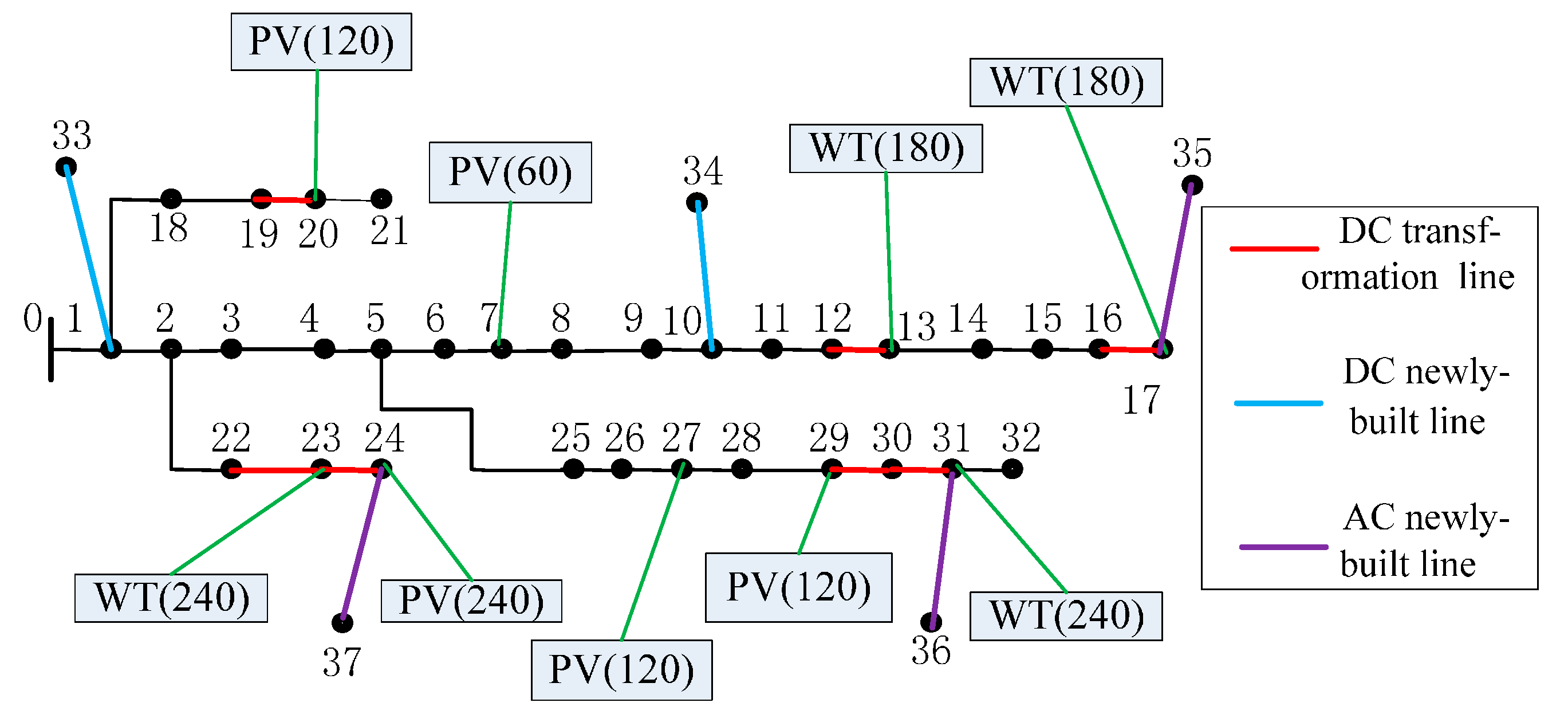
DG Configuration
(Node (DG Types, DG Capacity (kVA)))
DG Capacity (kVA)DC Line TransformationNewly Built DC Line
7 (PV, 60)
13 (WT, 180)
17 (WT, 180)
20 (PV, 120)
23 (WT, 240)
24 (PV, 240)
27 (PV, 120)
29 (PV, 120)
31 (WT, 240)
WT: 840
PV: 660
Total capacity: 1500
12–13
16–17
19–20
22–23
23–24
29–30
30–31
33–1 (AC)
34–10 (AC)
35–17 (DC)
36–31 (DC)
37–24 (DC)
Table 4. The objective function values when considering DC line transformation and newly built DC line.
Each Objective ItemNumerical Value
Annual investment, operational and maintenance costs of the DG (million yuan)146.34
The DC line transformation and newly built DC line costs (million yuan)1.325
The converter of grid-connected DG cost (million yuan)0.32
The converter of load connected cost (million yuan)3.102
The converter on DC line cost (million yuan)26.6
Annual economic cost (million yuan)177.6870
Annual active network loss (MW·h)884.12
Annual average voltage stability index0.062
Table 5. The planning results without considering DC line transformation and newly built DC line.
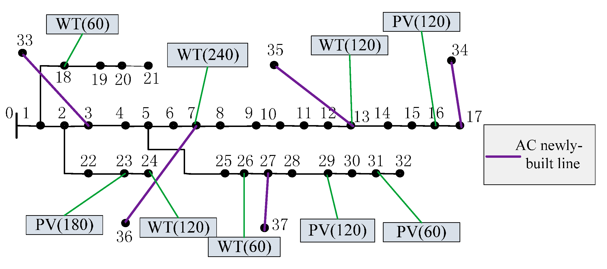
DG Configuration
(Node (DG types, DG Capacity (kVA)))
DG Capacity (kVA)DC line TransformationNewly Built DC Line
7 (WT, 240)
13 (WT, 120)
16 (PV, 120)
18 (WT, 60)
23 (PV, 180)
24 (WT, 120)
26 (WT, 60)
29 (PV, 120)
31 (PV, 60)
WT:600
PV:480
Total capacity: 1080
/33–3 (AC)
34–17 (AC)
35–13 (AC)
36–7 (AC)
37–27 (AC)
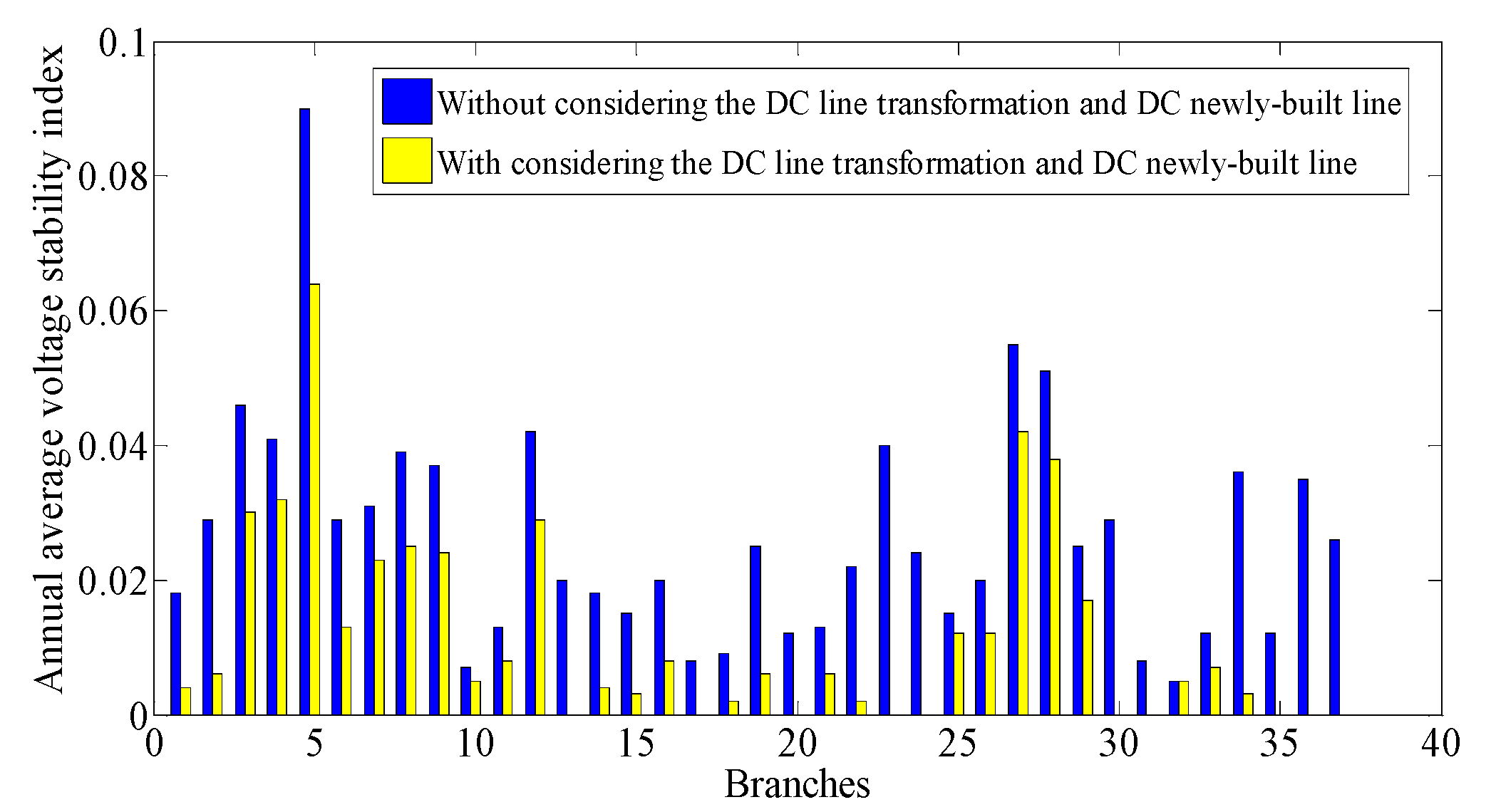
Table 6. The objective function values when considering the DC planning scheme.
Each Objective ItemConsidering DC Line Transformation and Newly Built DC LineIgnoring DC Line Transformation and Newly Built DC Line
Annual investment, operational and maintenance costs of the DG (million yuan)146.34134.92
The DC line transformation and newly built DC line costs (million yuan)1.3251.283
The converter of grid-connected DG cost (million yuan)0.3223.34
The converter of load connected cost (million yuan)3.10224.245
The converter on DC line cost (million yuan)26.60
Annual economic cost (million yuan)177.6870183.7880
Annual active network loss (MW·h)884.121223.45
Annual average voltage stability index0.0620.091

