Boolean Network-Based Sensor Selection with Application to the Fault Diagnosis of a Nuclear Plant

Abstract

Fault diagnosis is crucial for the operation of energy systems such as nuclear plants, and heavily relies on various types of sensors for temperature, pressure, concentration, etc. Due to the redundancy of sensors in each energy system, the sensor selection scheme can deeply influence the diagnostic efficiency. In this paper, a Boolean network (BN) with its linear representation is proposed for describing the fault propagation among sensors. Both the sufficient condition of fault detectability and that of fault discriminability are given. Then, a sensor selection method for fault detection and discrimination is proposed. Finally, the theoretic result is applied to realize the diagnosis oriented sensor selection for a nuclear steam supply system based on a modular high temperature gas-cooled reactor (MHTGR). The computation and simulation results verify the correctness of the theoretical results.

1. Introduction

Process behavior is inferred by using sensors measuring the important variables in processes such as those of nuclear and fossil thermal plants. When a process encounters a fault, the effect of this fault is propagated to all or some of the process variables. The main objective of fault diagnosis is to observe these fault symptoms and determine the root cause for the behavior, and the efficiency of fault diagnosis depends critically on the selection of sensors monitoring the process variables. Directed graph (DG) is one such qualitative model that can be used to infer the fault propagation or cause-effect behavior in a process system. Sensor selection was treated as different DG-based optimization problems in most early studies. Bagajewicz et al. summarized the sensor selection in a process as mix integer linear programming (MILP) problems focusing on optimizing cost or (and) reliability [1,2,3,4]. Bhushan, Narasimhan, and Rengaswamy added the criteria of robustness to the MILP problems [5]. Genetic algorithms (GAs) were also applied to solve the optimization problems for sensor selection [6,7]. The MILP approach has been applied to the sensor selection problem of the fault diagnosis for integral pressurized water reactors (iPWRs) and helical coil steam generators [8,9].

Boolean network (BN), first introduced by Kauffman [10], has been a powerful tool in modeling and analyzing cellular networks. A BN is a network with nodes and directed edges, where the state of a node is quantized to the values of True or False, and is determined through logical rules by the states of other nodes with edges directed to this node. It was shown that BN plays a crucial role in modeling cell regulation [10]. BN can be also applied to other fields such as system sciences as a powerful tool. Cheng and Qi gave the state-space model of BN based on its linear representation, and then revealed some features such as fix points, cycles, and controllability [11,12,13,14].

In this paper, by regarding both the sensors and faults in a process as the nodes in a BN, and by further regarding the cause effect behaviors as the directed edges, the BN is utilized as a qualitatively modeling the fault propagation of a process system. Then, the sensor selection problem for fault diagnosis is solved by analyzing the steady state-space structure of this BN model, and the sufficient conditions for both fault detection and fault discrimination are proposed. The implementation strategy of this BN-based sensor selection method for fault diagnosis are also given. Finally, this BN-based sensor selection method is applied to realize fault detection and discrimination of a Modular High Temperature Gas-cooled Reactor (MHTGR)-based nuclear steam supplying system, and the corresponding computation and simulation results show the feasibility of this new approach.

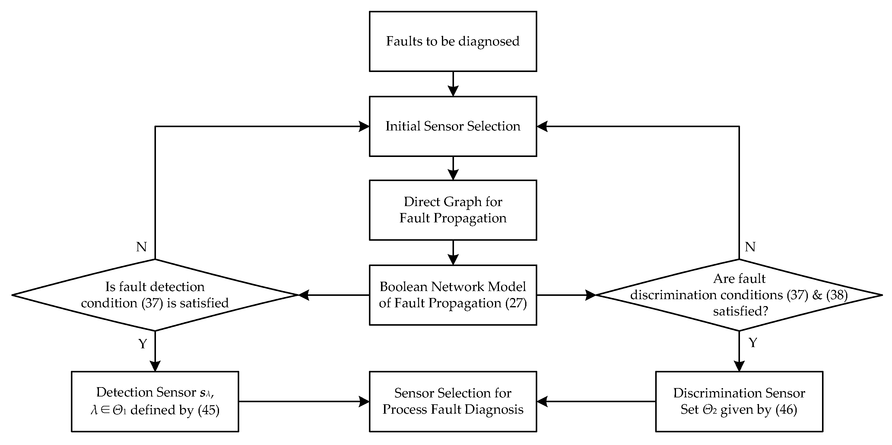
2. BN-Based Sensor Selection Method

2.1. Semi-Tensor Product and Logics

In this section, some definitions and lemmas about the semi-tensor product and logical function are introduced or given as follows with some necessary remarks.

Definition 1

[11,12]. Suppose A ∈ M_m×n and B ∈ M_p×q, and let t be the lowest common multiple (LCM) of positive integers n and p. The semi-tensor product (STP) of A and B is defined by:

$$A⊳<B=\left(A\otimes I_{t/n}\right)\left(B\otimes I_{t/p}\right)$$

(1)

where $\otimes$ is the Kronecker product, and I is the identity matrix.

Remark 1.

The semi-tensor product is the generalization of traditional matrix multiplication. In the following parts of this paper, symbol “$⊳<$” is omitted.

Definition 2

[13]. Matrix A ∈ M_m×n is called a logical matrix if the columns of A, denoted by Col(A), satisfy Col(A) $\subset$ Δ_m, where Δ_m = {${\delta }_m^k$| k = 1, …, m}, and ${\delta }_m^k$ is the kth column of I_m. The set of m × n logical matrices is denoted by L_m×n, and Δ₂ is usually denoted by Δ.

Definition 3

[13]. W_[m,n] ∈ M_mn×mn is called a swap matrix if its column labels are given by (11, …, 1n, …, m1, …, mn), its row labels are given by (11, …, m1, …, 1n, …, mn), and its element in position (IJ, ij) is given by:

$$w_{IJ,ij}=\{\begin{array}{cc}1,& I=i,J=j,\\ 0,& \mathrm{otherwise}.\end{array}$$

(2)

Moreover, W_[n,n] is briefly denoted as W_[n].

Lemma 1

[13,14]. Let x ∈ R^m, y ∈ Rⁿ, and A ∈ M_p×q. Then:

$$W_{\left[m,n\right]}xy=yx$$

(3)

$$xA=\left(I_m\otimes A\right)x$$

(4)

Definition 4

[13]. A 2 × 2ⁿ matrix M_σ is called structure matrix of a logical function σ: Δⁿ→Δ, if

$$\sigma \left(a_1,a_2,\dots ,a_n\right)=M_{\sigma }{a}_1{a}_2\cdots a_n$$

(5)

where a_i ∈ Δ, i = 1, 2, …, n.

For example, the power-reducing matrix M_r is defined by:

$$a^2=aa=M_{\mathrm{r}}a$$

(6)

where

$$M_{\mathrm{r}}=\left[\begin{array}{cc}{\delta }_4^1& {\delta }_4^4\end{array}\right]:={\delta }_4\left[\begin{array}{cc}1& 4\end{array}\right]$$

(7)

Based on the power-reducing matrix and swap matrices, the following lemma can be obtained.

Lemma 2

[13]. Every logical function σ: Δⁿ→Δ has a structure matrix M_σ ∈ L_2×2ⁿ satisfying Equation (5).

Remark 2.

The structure matrices of logical functions negation “¬”, disjunction “∨” and conjunction “∧” are given by:

$$M_{\neg }={\delta }_2\left[\begin{array}{cc}2& 1\end{array}\right]$$

(8)

$$M_{\vee }={\delta }_2\left[\begin{array}{cccc}1& 1& 1& 2\end{array}\right]$$

(9)

$$M_{\wedge }={\delta }_2\left[\begin{array}{cccc}1& 2& 2& 2\end{array}\right]$$

(10)

respectively. Moreover, the logical functions of identity “I” and constant “F” have the structure matrices given by:

$$M_{\mathrm{I}}={\delta }_2\left[\begin{array}{cc}1& 2\end{array}\right]=I_2$$

(11)

$$M_{\mathrm{F}}={\delta }_2\left[\begin{array}{cc}2& 2\end{array}\right]$$

(12)

respectively.

Let A_n = a₁, a₂, …, a_n, where a_i ∈ Δ and i = 1,…, n. The following lemma gives the relationship between $A_n^2$ and A_n, which is newly proposed in this paper.

Lemma 3.

For A_n = a₁, a₂, …, a_n, where a_i ∈ Δ, i = 1, …, n. Then:

$$A_n^2={\Phi }_n{A}_n$$

(13)

where

$${\Phi }_n=\mathrm{diag}\left({\delta }_{2^n}^1,\cdots ,{\delta }_{2^n}^{2^n}\right)$$

(14)

and ${\delta }_{2^n}^k\in {\Delta }_{2^n},k=1,\cdots ,2^n.$

Proof. 

Since a_i ∈ Δ, i.e., a_i = [10]^T or [01]^T (i = 1, …, n), from Definition 1, it can be seen that:

$$A_n=a_1{a}_2\dots a_n={\delta }_{2^n}^k$$

(15)

Also from Definition 1,

$$A_n^2=\left(A_n\otimes I_{2^n}\right)A_n=\left({\delta }_{2^n}^k\otimes I_{2^n}\right){\delta }_{2^n}^k=\left[\begin{array}{c}{O}_{\left(k-1\right)2^n\times 2^n}\\ I_{2^n}\\ O_{\left(2^n-k\right)2^n\times 2^n}\end{array}\right]{\delta }_{2^n}^k=\left[\begin{array}{c}{O}_{\left(k-1\right)2^n\times 1}\\ {\delta }_{2^n}^k\\ O_{\left(2^n-k\right)2^n\times 1}\end{array}\right]$$

(16)

Moreover, it can be directly derived that:

$$\left[\mathrm{diag}\left({\delta }_{2^n}^1,\cdots ,{\delta }_{2^n}^{2^n}\right)\right]{\delta }_{2^n}^k=\left[\begin{array}{ccccccccc}{\delta }_{2^n}^1& O_{2^n\times 1}& \cdots & O_{2^n\times 1}& O_{2^n\times 1}& O_{2^n\times 1}& \cdots & O_{2^n\times 1}& O_{2^n\times 1}\\ O_{2^n\times 1}& {\delta }_{2^n}^2& \cdots & O_{2^n\times 1}& O_{2^n\times 1}& O_{2^n\times 1}& \cdots & O_{2^n\times 1}& O_{2^n\times 1}\\ ⋮& ⋮& ⋮& ⋮& ⋮& ⋮& ⋮& ⋮& ⋮\\ O_{2^n\times 1}& O_{2^n\times 1}& \cdots & {\delta }_{2^n}^{k-1}& O_{2^n\times 1}& O_{2^n\times 1}& \cdots & O_{2^n\times 1}& O_{2^n\times 1}\\ O_{2^n\times 1}& O_{2^n\times 1}& \cdots & O_{2^n\times 1}& {\delta }_{2^n}^k& O_{2^n\times 1}& \cdots & O_{2^n\times 1}& O_{2^n\times 1}\\ O_{2^n\times 1}& O_{2^n\times 1}& \cdots & O_{2^n\times 1}& O_{2^n\times 1}& {\delta }_{2^n}^{k+1}& \cdots & O_{2^n\times 1}& O_{2^n\times 1}\\ ⋮& ⋮& ⋮& ⋮& ⋮& ⋮& ⋮& ⋮& ⋮\\ O_{2^n\times 1}& O_{2^n\times 1}& \cdots & O_{2^n\times 1}& O_{2^n\times 1}& O_{2^n\times 1}& \cdots & {\delta }_{2^n}^{2^n-1}& O_{2^n\times 1}\\ O_{2^n\times 1}& O_{2^n\times 1}& \cdots & O_{2^n\times 1}& O_{2^n\times 1}& O_{2^n\times 1}& \cdots & O_{2^n\times 1}& {\delta }_{2^n}^{2^n}\end{array}\right]\left[\begin{array}{c}0\\ 0\\ ⋮\\ 0\\ 1\\ 0\\ ⋮\\ 0\\ 0\end{array}\right]=\left[\begin{array}{c}{O}_{\left(k-1\right)2^n\times 1}\\ {\delta }_{2^n}^k\\ O_{\left(2^n-k\right)2^n\times 1}\end{array}\right]$$

(17)

From Equations (15)–(17):

$$A_n^2=\left[\mathrm{diag}\left({\delta }_{2^n}^1,\cdots ,{\delta }_{2^n}^{2^n}\right)\right]{\delta }_{2^n}^k$$

(18)

which means that Equation (14) is well satisfied, which proves Lemma 3. ☐

Remark. 3.

For n = 1, from Equations (6), (7) and (14), it can be seen that:

$${\Phi }_1=\mathrm{diag}\left(\begin{array}{cc}{\delta }_2^1& {\delta }_2^2\end{array}\right)=\left[\begin{array}{cc}{\delta }_4^1& {\delta }_4^4\end{array}\right]=M_{\mathrm{r}}$$

(19)

From Equation (19), Φ_n given by Equation (14) can be regarded as an extension of matrix M_r defined by Equation (7).

2.2. BN Model of Fault Propagation and Its Linear Representation

The nodes of a directed graph (DG) describing fault propagation is composed of faults f_i ∈ Δ and sensors s_j ∈ Δ, i = 1,…, m, j = 1,…, n. The edge from fault f_i to sensor s_j denotes that f_i can be detected by s_j. The edge from sensors s_j to s_k reveals the fault-propagation between the process variables measured by these two sensors. It is assumed that there are no edges between any two faults. There may be several edges toward a sensor node, whose logical operation among the start nodes of these edges should be disjunction.

For convenience of discussion, define matrices E_SF = {e_SF,ji} ∈ M_n×m and E_SS = {e_SS,kl} ∈ M_n×n, where i = 1, …, m and j, k, l = 1,…, n. Here, e_SF,ji = 1 if there exists an edge from fault f_i to sensor s_j, e_SS,kl = 1 if there is an edge from s_l to s_k, otherwise e_SF,ji = 0 and e_SS,kl = 0. It is worth noting that matrices are determined by the physical and thermal-hydraulic features of the under-considered processes.

Based on the above assumption and analysis about the features of the DG for process fault propagation, the BN model for fault propagation can be written as:

$$s_k\left(t+1\right)=M_{\vee }^{m+n-1}\left({\displaystyle \prod }_{i=1}^m{M}_{\mathrm{F},i}{f}_i\right)\left[{\displaystyle \prod }_{j=1}^n{M}_{\mathrm{S},j}{s}_j\left(t\right)\right],$$

(20)

where k = 1, …, n, t is the times of logic computation,

$$M_{\mathrm{F},i}=\{\begin{array}{cc}{M}_{\mathrm{I}},& e_{\mathrm{SF},ki}\ne 0,\\ M_{\mathrm{F}},& e_{\mathrm{SF},ki}=0,\end{array}$$

(21)

$$M_{\mathrm{S},j}=\{\begin{array}{cc}{M}_{\mathrm{I}},& e_{\mathrm{SS},kj}\ne 0,\\ M_{\mathrm{F}},& e_{\mathrm{SS},kj}=0,\end{array}$$

(22)

matrices M_∨, M_I, and M_F are defined by Equations (9), (11), and (12), respectively, f_i, s_j ∈ Δ, and here e_SF,ki and e_SS,kj (i = 1, …, m; j, k = 1, …, n) are respectively the entries of matrices E_SF and E_SS.

Based on Equations (4) and (20):

$$s_k\left(t+1\right)=L_k{\displaystyle \prod }_{i=1}^m{f}_i{\displaystyle \prod }_{j=1}^n{s}_j\left(t\right),$$

(23)

where

$$L_k=M_{\vee }^{m+n-1}\left\{\left[{\displaystyle \prod }_{i=1}^m\left(I_{2^{i-1}}\otimes M_{\mathrm{F},i}\right)\right]\left[{\displaystyle \prod }_{j=1}^n\left(I_{2^{m+j-1}}\otimes M_{\mathrm{S},j}\right)\right]\right\}$$

(24)

Define

$$S\left(t\right)={\displaystyle \prod }_{j=1}^n{s}_j\left(t\right)=s_1\left(t\right)s_2\left(t\right)\cdots s_n\left(t\right)$$

(25)

And

$$F={\displaystyle \prod }_{i=1}^{m}f=f_1{f}_2\cdots f_m$$

(26)

The state-space model of BN describing process fault propagation is proposed by the following theorem, which is the first main result of this paper.

Theorem 1.

The state-space model of the BN for process fault propagation given by Equation (23) is:

$$S\left(t+1\right)=L_{\mathrm{F}}S\left(t\right)$$

(27)

where

$$L_{\mathrm{F}}=LF$$

(28)

$$L=L_1{\displaystyle \prod }_{k=2}^n\left[\left(I_{2^{m+n}}\otimes L_k\right){\Phi }_{m+n}\right]$$

(29)

L_k and Φ_m+n are given by Equations (24) and (14), respectively.

Proof. 

From Lemma 3:

$${\left[FS\left(t\right)\right]}^2={\Phi }_{m+n}FS\left(t\right)$$

(30)

Based on Equations (23) and (25):

$$\begin{array}{cc}S\left(t+1\right)& =L_{1}FS\left(t\right)L_{2}FS\left(t\right){\displaystyle \prod }_{k=3}^n{L}_{k}FS\left(t\right)\hfill \\ & =L_1\left[\left(I_{2^{m+n}}\otimes L_2\right){\Phi }_{m+n}\right]FS\left(t\right){\displaystyle \prod }_{k=3}^n{L}_{k}FS\left(t\right)\hfill \\ & =\cdots \hfill \\ & =L_1{\displaystyle \prod }_{k=2}^n\left[\left(I_{2^{m+n}}\otimes L_k\right){\Phi }_{m+n}\right]FS\left(t\right)，\hfill \end{array}$$

(31)

which completes the proof of this theorem. ☐

Remark 4.

From Equation (27), it is easy to see that L_F = LF is a 2ⁿ × 2ⁿ matrix which is called sensor network state transition matrix. Fault F is regarded as a constant vector which is the parameter of state transition matrix.

Remark 5.

For f_i, s_j ∈ Δ (i = 1, …, m; j = 1,…, n), it can be seen directly from Equations (25) and (26) that F ∈ ${\Delta }_{2^m}$ and S ∈ ${\Delta }_{2^n}$.

2.3. Sufficient Conditions of Fault Detectability and Discriminability

Based on the definition of semi-tensor product, the following lemma can be obtained directly.

Lemma 4

[13]. Consider A_n = a₁, a₂, …, a_n, where a_i = [Q_i 1 − Q_i]^T ∈ Δ, Q_i ∈ {0, 1}, and i = 1, 2, …, n. If A_n = ${\delta }_{2^n}^k$ (k = 1, …, 2ⁿ), then:

$$k=2^n-{\displaystyle \sum _{i=1}^n{Q}_i{2}^{n-i}}$$

(32)

Then, the fault detectability and discriminability of a BN is given by Theorem 2, which is the second main result of this paper.

Theorem 2.

Consider BN model Equation (27) for process fault propagation. Suppose that only one fault occurs at a time. For each i = 1, 2, …, m, it is assumed that there is a positive integer q_i such that:

$${\left(L{\delta }_{2^m}^{k_i}\right)}^{q_i+1}={\left(L{\delta }_{2^m}^{k_i}\right)}^{q_i}$$

(33)

where

$$k_i=2^m-2^{m-i}$$

(34)

Define

$$P=\left[\begin{array}{cccc}{p}_1& p_2& \cdots & p_m\end{array}\right]$$

(35)

where

$$p_i={\left(L{\delta }_{2^m}^{k_i}\right)}^{q_i}{S}_0$$

(36)

i = 1, …, m, and S₀ ∈ ${\Delta }_{2^n}$. For initial sensor state S(0) = S₀, fault f_i (i ∈ {1, …, m}) is detectable if

$$p_i\ne {\delta }_{2^n}^{2^n}$$

(37)

Furthermore, all the faults are discriminable if both conditions Equation (37) and

$$\mathrm{Rank}\left(P\right)=m$$

(38)

are satisfied, where the value of function Rank(P) is the rank of matrix P defined by Equation (35) .

Proof. 

For a given i ∈ {1, 2, …, m}, i.e., F = ${\delta }_{2^m}^{k_i}$ with k_i given by Equation (34). Then, from BN model Equation (27):

$$S\left(t\right)={\left(LF\right)}^t{S}_0={\left(L{\delta }_{2^m}^{k_i}\right)}^t{S}_0$$

(39)

If there exists a positive integer q_i so that Equation (33) is well satisfied, then the steady response of the BN to fault i corresponding to initial sensor state S₀ is:

$$S\left(q_i\right)={\left(L{\delta }_{2^m}^{k_i}\right)}^{q_i}{S}_0$$

(40)

If there is no sensor response to fault f_i, the steady response of the BN should be ${\delta }_{2^n}^{2^n}$. Thus, if

$${\left(L{\delta }_{2^m}^{k_i}\right)}^{q_i}{S}_0\ne {\delta }_{2^m}^{2^m}$$

(41)

holds for each i ∈ {1, 2, …, m}, i.e., condition Equation (37) is satisfied, then the faults are detectable. ☐

Moreover, suppose

$$p_r\ne p_s$$

(42)

for r ≠ s and r, s ∈ {1, 2, …, m}, i.e., the condition Equation (38) is satisfied. It is easy to see from Inequality (42) that the steady responses of the sensor state to different faults are different from each other, which means that the faults are discriminable, i.e., the faults can be identified, which proves Theorem 2.

Remark 6.

For i ∈ {1, 2, …, m}, there is an integer l_i ∈ {1, …, 2ⁿ}, so that:

$${\delta }_{2^n}^{l_i}={\left(L{\delta }_{2^m}^{k_i}\right)}^{q_i}{S}_0$$

(43)

Define

$${\Pi }_i=\left\{\begin{array}{cc}r\in \mathrm{N}|& 2^n-l_i={\displaystyle \sum _{r=1}^n{Q}_r{2}^{n-r}},Q_r\ne 0\end{array}\right\}$$

(44)

which is the collection of sensors having respond to fault i. Let

$${\Theta }_1=\underset{i=1}{\overset{m}{{\displaystyle \cap }}}{\Pi }_i$$

(45)

If Θ₁ is not empty, then we can use sensor s_λ with λ ∈ Θ₁ for fault detection, and use sensors in the set

$${\Theta }_2=\underset{i=1}{\overset{m}{{\displaystyle \cup }}}{\Pi }_i-{\Theta }_1$$

(46)

for fault discrimination.

Remark 7.

The practical implementation steps of the BN-based sensor selection method for process fault detection and discrimination are summarized in Figure 1. After the measurement system design, the sensor network is given. For diagnosing a set of process faults, an initial sensor selection can be given. Then, it should be verified whether this sensor selection is proper for fault detection and discrimination. Based upon the physical and thermal-hydraulic features of the process, the DG for fault propagation can be determined. Then, the linear representation of the BN model of fault propagation (Equation (27)) can be obtained. By verifying both the conditions of fault detection (Equation (37)) and discrimination (Equation (38)), it can be seen that the sensor network is reasonable for fault diagnosis. If either conditions of Equations (37) or (38) are not satisfied, then the measurement system should be redesigned. Otherwise, we can use a sensor contained in set Θ₁ given by Equation (45) for fault detection, and further use the sensors in set Θ₂ given by Equation (46) for fault discrimination.

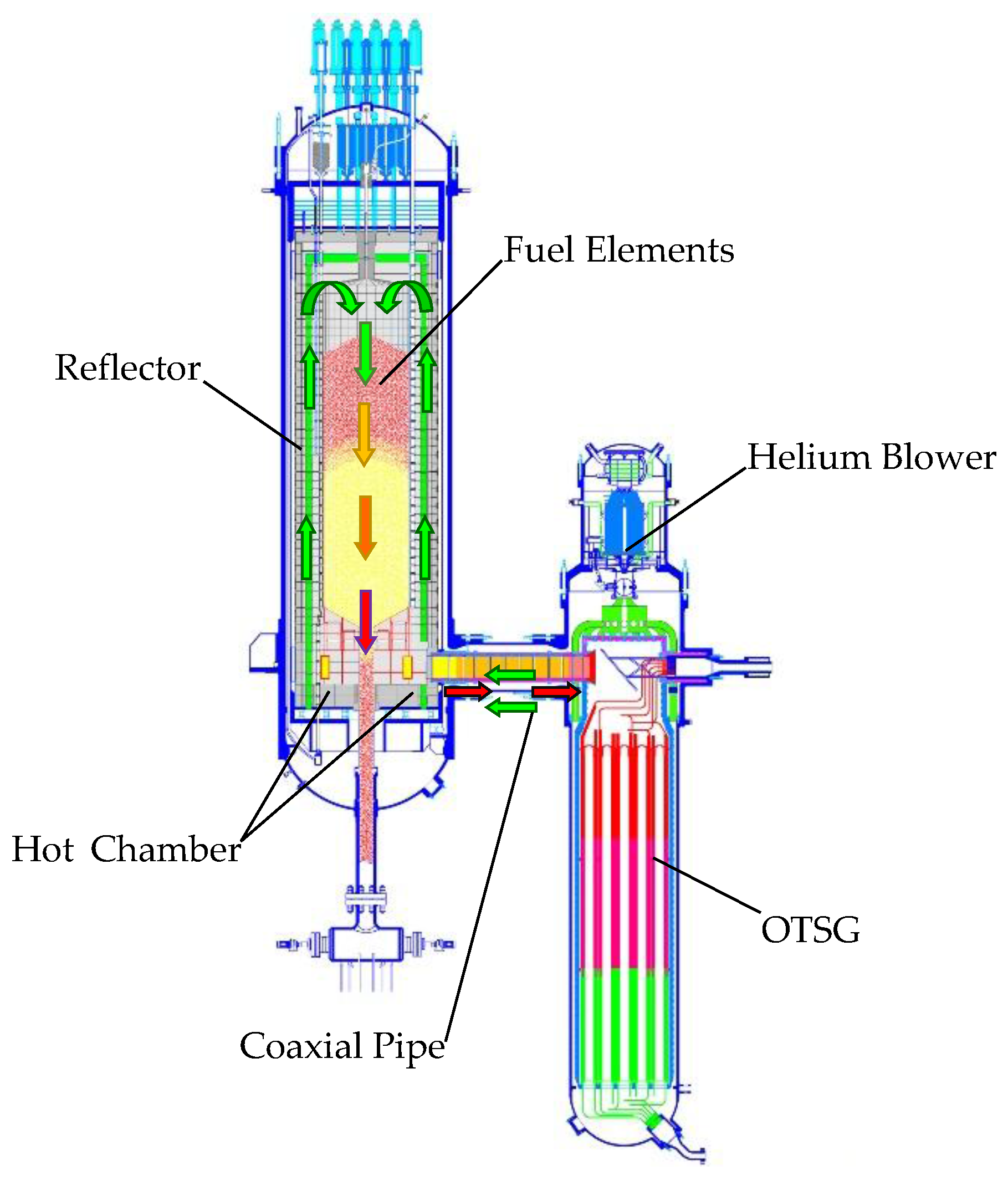
3. Application to a High Temperature Gas-Cooled Reactor Nuclear Plant

The BN model and its linear representation for process fault propagation given by Theorem 1, the sufficient conditions for fault detectability and discriminability given by Theorem 2, and the sensor selection method proposed in Remark 6 are applied to realize a fault diagnosis-oriented sensor selection of a nuclear steam supply system (NSSS) based on a modular high temperature gas-cooled reactor (MHTGR).

3.1. Background

The modular high temperature gas-cooled reactor (MHTGR) adopts helium as a coolant and graphite as both a moderator and structural material. Due to its inherent safety feature that is given by low power density, strong temperature-induced reactivity feedback, and large surface-to-volume ratio, the MHTGR has already been accepted as one of the best candidates for the next generation of nuclear plants. Figure 2 shows a schematic diagram of an MHTGR-based NSSS module of the under-constructed two modular High Temperature gas-cooled Reactor Pebble-bed Module (HTR-PM) plant [15]. This NSSS module is composed of an MHTGR, a helical-coil once-through steam generator (OTSG), a helium blower, and some necessary vessels and pipes. It can be seen from Figure 2 that the cold helium enters the helium blower mounted on top of the OTSG, and is then pressurized before flowing into the cold gas duct. The cold helium enters into the channels in the side-reflector from bottom to top for cooling the reflector, and then passes through the pebble-bed from top to bottom, where it is heated to a high temperature of about 750 °C. The hot helium leaves the hot gas chamber inside the bottom reflector and flows into the OTSG primary side, where it is cooled by the secondary water/steam flow.

Fault diagnosis of the NSSS is necessary to improve the operation reliability of an MHTGR-based nuclear plant. Sensor selection is necessary for satisfactory diagnosis. The sensors to be selected are those measuring the reactor neutron flux, primary helium flowrate, secondary feedwater flowrate, and average coolant temperatures of the primary and secondary sides, which are all given in

Table 1. Available sensor nodes for selection.

Nodes	Description	Unit	Range	Precision	Output Signal
s1	reactor neutron flux	%	0~200	2	4~20 mA
s2	primary helium flowrate	kg/s	0~200	2	4~20 mA
s3	average temperature of the primary flow	°C	300~700	1	4~20 mA
s4	average temperature of the secondary flow	°C	330~430	0.5	4~20 mA

with the measurement range and precision as well as the type of sensor output signal. The measurement range of each sensor corresponds with the output range of 4~20 mA. The faults to be detected or discriminated are given in

Table 2. Fault nodes to be detected or discriminated.

Nodes	Description
f1	abnormal reactivity injection to the reactor
f2	malfunction of the primary helium blower
f3	heat transfer degradation of OTSG two sides

, which include the abnormal reactivity injection, malfunction of the primary helium blower, and heat transfer degradation between the two sides of the OTSG.

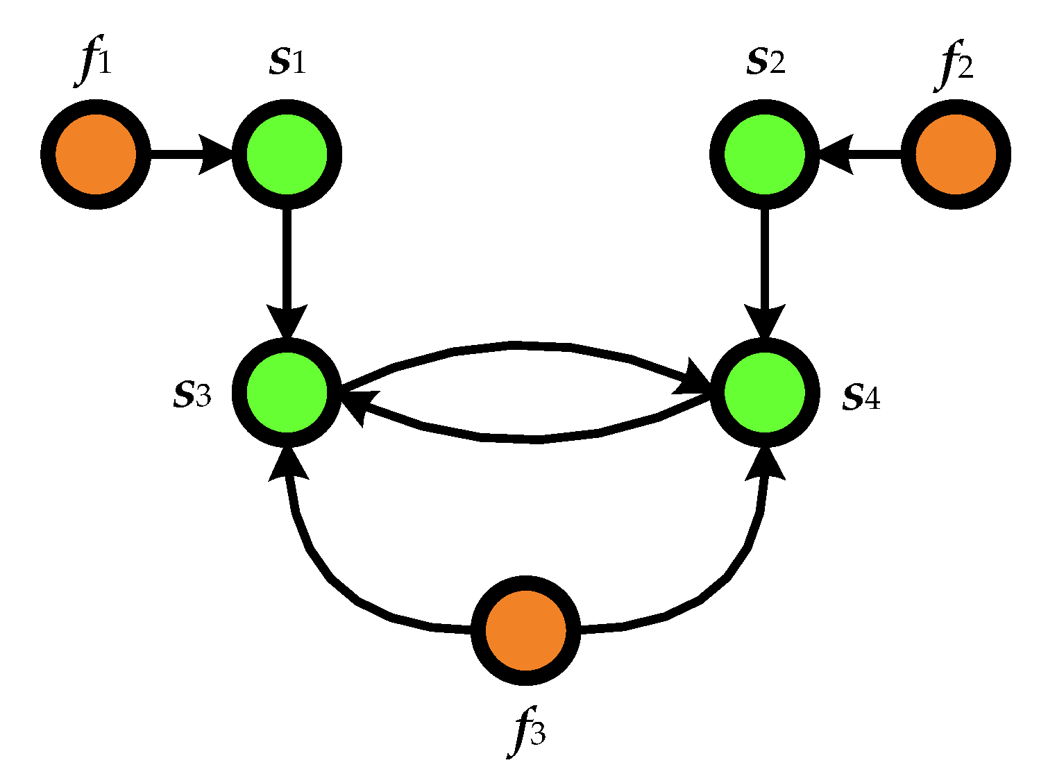
3.2. Directed Graph for Fault Propagation

From the physical and thermal-hydraulic features of the MHTGR-based NSSS, the following relationships between fault f_i (i = 1, 2, 3) and sensor s_j (j = 1, 2, 3, 4) can be observed:

(1)

If fault f₁ occurs, i.e., there is an abnormal positive or negative reactivity injection, then the neutron flux is abnormal, which further leads to abnormality in the acquired signal by s₁. Since the variation of neutron flux can directly result in the variations of primary coolant temperature, fault f₁ can also lead to abnormality in the acquired signal by s₃. As the variation of the primary helium temperature can result in that of secondary coolant temperature, abnormality in the acquired signal by s₃ can further lead to that of sensor s₄.

(2)

If fault f₂ occurs, i.e., the primary helium blower malfunctions, then there must be abnormality in the primary helium flowrate, which induces abnormality in the acquired signal by s₂. Since the steam temperature is very sensitive to the helium flowrate, abnormality in the acquired signal by s₂ can further lead to that of sensor s₄. Because the temperature of the secondary steam/water flow can influence the primary helium temperature, abnormality in the acquired signal by s₄ can induce that of s₃.

(3)

If fault f₃ occurs, i.e., the heat transfer between the two sides the OTSG will be degraded, then the thermal resistance of the OTSG becomes abnormal, which immediately leads to abnormalities of sensors s₃ and s₄. Here, fault f₃ may be induced by the limescale inside the tubes of the OTSG.

(4)

Since helium is transparent to the nuclear fission reaction, i.e., it has no temperature feedback effect to neutron flux, abnormality in the signal acquired by s₃ cannot directly induce that of s₁.

Based on the above four observations, the DG for fault propagation of the MHTGR-based NSSS can be shown by Figure 3.

3.3. BN Model of Fault Propagation and Its Linear Representation

The BN model for the fault propagation is:

$$\{\begin{array}{l}{s}_1\left(t+1\right)=f_1,\\ s_2\left(t+1\right)=f_2,\\ s_3\left(t+1\right)=f_3\vee s_1\left(t\right)\vee s_4\left(t\right),\\ s_4\left(t+1\right)=f_3\vee s_2\left(t\right)\vee s_3\left(t\right).\end{array}$$

(47)

From Theorem 1, the linear representation of model Equation (47) can be rewritten as:

$$S\left(t+1\right)=LFS\left(t\right)$$

(48)

where

$$\begin{array}{cccccccccccccccccc}L={\delta }_{16}[& 1& 1& 1& 1& 1& 1& 1& 1& 1& 1& 1& 1& 1& 1& 1& 1& \\ & 1& 1& 1& 1& 1& 1& 2& 2& 1& 3& 1& 3& 1& 3& 2& 4& \\ & 5& 5& 5& 5& 5& 5& 5& 5& 5& 5& 5& 5& 5& 5& 5& 5& \\ & 5& 5& 5& 5& 5& 5& 6& 6& 5& 7& 5& 7& 5& 7& 6& 8& \\ & 9& 9& 9& 9& 9& 9& 9& 9& 9& 9& 9& 9& 9& 9& 9& 9& \\ & 9& 9& 9& 9& 9& 9& 10& 10& 9& 11& 9& 11& 9& 11& 10& 12& \\ & 13& 13& 13& 13& 13& 13& 13& 13& 13& 13& 13& 13& 13& 13& 13& 13& \\ & 13& 13& 13& 13& 13& 13& 14& 14& 13& 15& 13& 15& 13& 15& 13& 15& ].\end{array}$$

(49)

3.4. Verification of Fault Detectability and Discriminability

From Equation (34), k₁ = 4, k₂ = 6, and k₃ = 7.

Furthermore, since

$$L_{\mathrm{F}1}=L{F}_1=L{\delta }_8^4={\delta }_{16}\begin{array}{cccccccccccccccccc}[& 5& 5& 5& 5& 5& 5& 6& 6& 5& 7& 5& 7& 5& 7& 6& 8& ]\end{array}$$

(50)

$$L_{\mathrm{F}2}=L{F}_2=L{\delta }_8^6={\delta }_{16}\begin{array}{cccccccccccccccccc}[& 9& 9& 9& 9& 9& 9& 10& 10& 9& 11& 9& 11& 9& 11& 10& 12& ]\end{array}$$

(51)

and

$$L_{\mathrm{F}3}=L{F}_3=L{\delta }_8^7={\delta }_{16}\begin{array}{cccccccccccccccccc}[& 13& 13& 13& 13& 13& 13& 13& 13& 13& 13& 13& 13& 13& 13& 13& 13& ],\end{array}$$

(52)

it can be verified that q₁ = q₂ = 3 and q₃ = 1, i.e.,

$$\begin{array}{ccc}{L}_{\mathrm{F}1}^4=L_{\mathrm{F}1}^3,& L_{\mathrm{F}2}^4=L_{\mathrm{F}2}^3,& L_{\mathrm{F}3}^2=L_{\mathrm{F}3}\end{array}$$

(53)

Consider initial state S₀ = ${\delta }_{16}^{16}$, which means that all the sensor states are ${\delta }_2^2$. Then,

$$P={\delta }_{16}\left[\begin{array}{ccc}5& 9& 13\end{array}\right]$$

(54)

From Equation (54), it can be seen that the matrix P satisfies the conditions of Equations (37) and (38), which certainly leads to both fault detectability and discriminability. Thus, the sensor network given by Table 1 is reasonable for fault diagnosis.

3.5. Sensor Selection

From Equation (43), l₁ = 5, l₂ = 9, and l₃ = 13. Then, from Equation (44):

$$\{\begin{array}{l}{\Pi }_1=\left\{1,3,4\right\},\\ {\Pi }_2=\left\{2,3,4\right\},\\ {\Pi }_3=\left\{3,4\right\}.\end{array}$$

(55)

Based upon Equation (50), sensor s₄ can be utilized to detect whether a fault belongs to the set S_F = {f₁, f₂, f₃} that occurs. Also from Equation (50), we obtain a reasonable fault discrimination strategy, i.e., sensor s₁ can be used to identify fault f₁, sensor s₂ can be used to identify fault f₂, and sensor s₃ can be used to identify fault f₃. Therefore, a rational sensor selection strategy, which satisfies the conditions of fault detection and discrimination given in Theorem 2, is obtained from Equation (50).

Moreover, it is worth noting here that the conditions given in Theorem 2 are sufficient conditions for fault detection and discrimination, which may thus provide a choice of multiple candidate fault diagnosis-oriented sensor selection strategies.

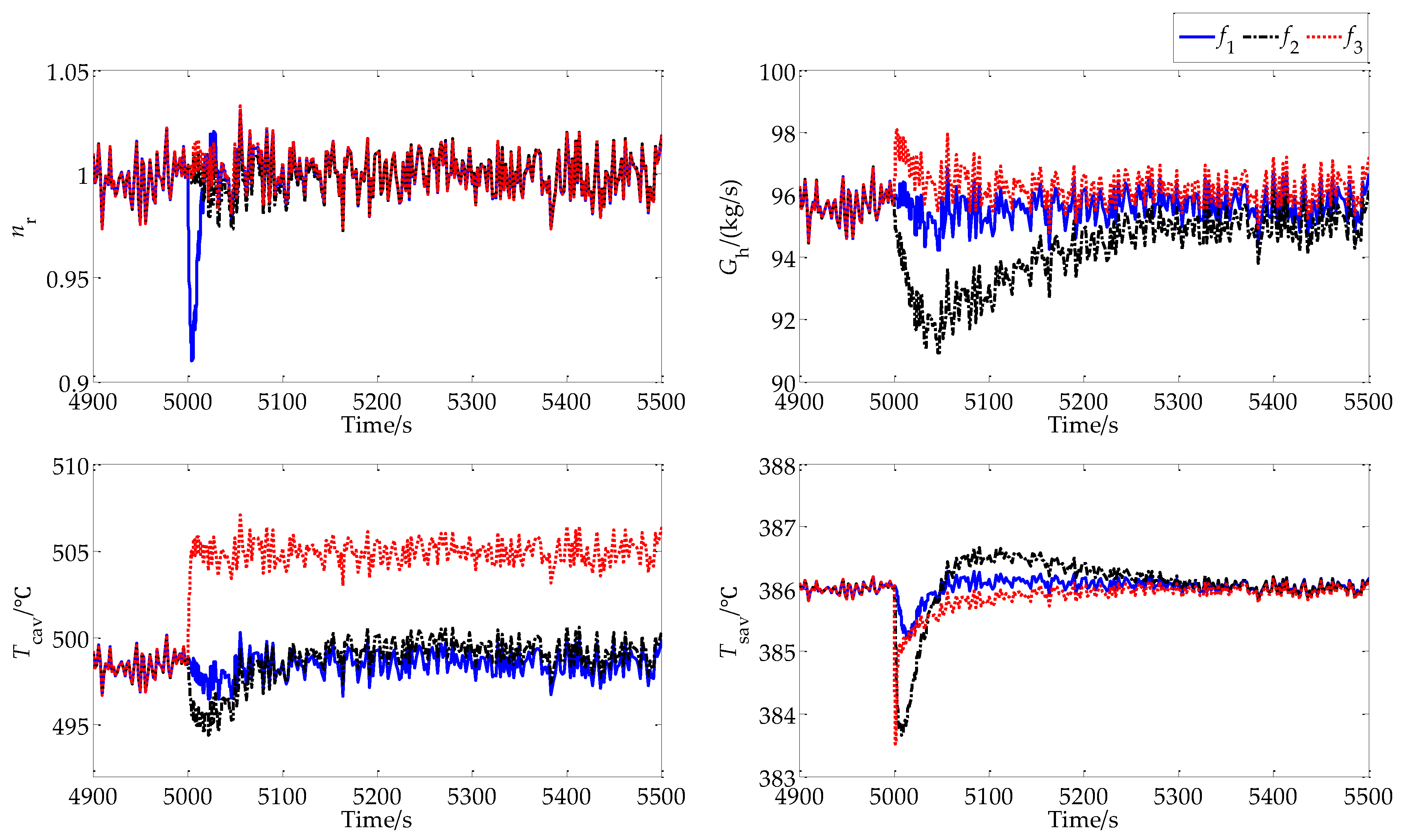
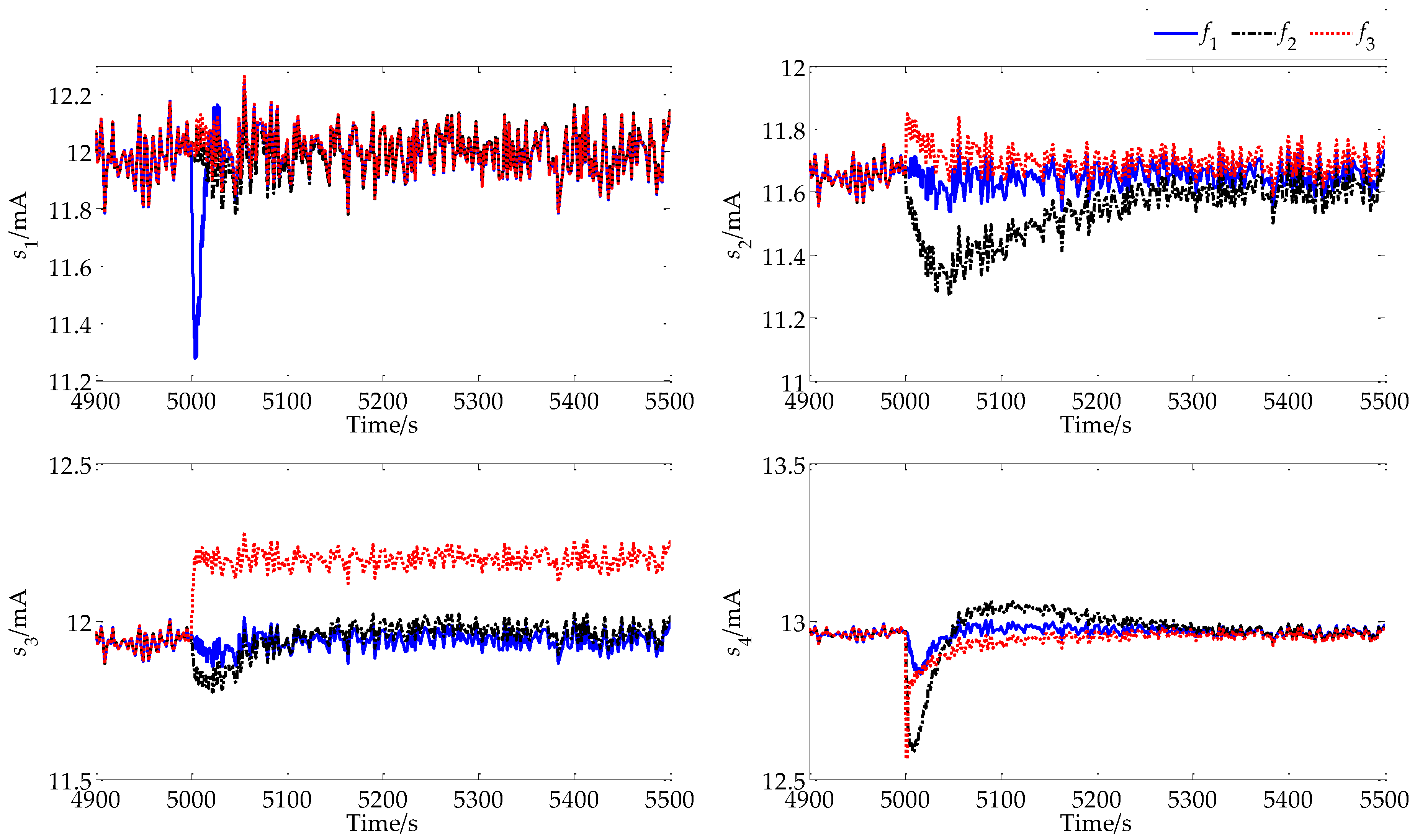
3.6. Numerical Simulation

The above sensor selection strategy for the fault diagnosis of the MHTGR-based NSSS module of an HTR-PM plant is verified by numerical simulation in full-scale simulation programs [16,17]. The power control of the NSSS adopts the model-free adaptive controller proposed in Reference [18], and the plant coordination control adopts the result given in References [19,20,21].

In this simulation, fault f₁ is simulated by injecting a negative step of reactivity with an amplitude of 0.1 $. Fault f₂ is simulated by a negative step decrease of a primary helium flowrate of 5 kg/s. Fault f₃ is simulated by stepping down the heat transfer coefficient between two sides of OTSG to 90% of its current value. Initially, the NSSS operates at full power, and a fault occurs at 5000 s. The responses of the normalized nuclear power n_r, primary helium flowrate G_h, average helium temperature of the MHTGR T_cav, and average temperature of the OTSG secondary coolant T_sav under faults f₁, f₂, and f₃ are all shown in Figure 4. Here, the responses of n_r, G_h, T_cav, and T_sav correspond to sensors s₁, s₂, s₃, and s₄, respectively. Since the output of sensor s_i (i = 1, 2, 3, 4) is the analogous signal of 4–20 mA, which is widely adopted in practical engineering, the responses of sensor outputs are shown in Figure 5. Here, the white noises added to the simulation are based on the measurement precision of the sensors given in Table 1.

Based on the comparison among the responses of n_r, G_h, T_cav, and T_sav as well as the output signal of sensor s_i (i = 1, 2, 3, 4) under faults f₁, f₂, and f₃, it can be seen that sensor s_i is sensitive to fault f_i (i = 1, 2, 3), and the sensitivity of s₄ to faults f₁, f₂, and f₃ are nearly the same. Thus, the fault diagnosis strategy of using s₄ for fault detection and using s_i (i = 1, 2, 3) for fault discrimination is reasonable, which verifies the correctness of the theoretic result. It is worth noting that, for fault discrimination, the output signal of s₁ is used to distinguish f₁ from f₂ and f₃, i.e., to identify f₁. However, the output signal of s₁ is not used to distinguish f₂ from f₃. This is the same for fault identification based on the output signals of sensors s₂ and s₃.

4. Conclusions

Since there are hundreds of sensors for temperature, pressure, concentration, etc. in complex process systems such as nuclear and chemical plants, and due to the fault propagation effect among these sensors, a proper sensor selection scheme is the basis for efficient process fault diagnosis. Sensor selection was treated as optimization problems under certain criteria. However, the precondition of conducting optimization is fault detectability and discriminability. In this paper, a Boolean network (BN) model in a linear representation is proposed for describing the fault propagation among sensors. Based on the analysis of the steady state-space structure of the BN model, sufficient conditions for both fault detectability and discriminability are given. According to these sufficient conditions, a sensor selection method for fault detection and discrimination is also proposed. Finally, the above result is applied to realize the fault diagnosis-oriented sensor selection for an MHTGR-based NSSS. Both the computation and simulation results verify the theoretical results.

References

1. Bagajewicz, M. Design and retrofit of sensor networks in process plants. AIChE J. 1997, 43, 2300–2306. [Google Scholar] [CrossRef]
2. Bagajewicz, M. A review of techniques for instrumentation and upgrade in process plants. Can. J. Chem. Eng. 2002, 80, 3–16. [Google Scholar] [CrossRef]
3. Bagajewicz, M.; Cabrera, E. New MILP formulation for instrumentation network design and upgrade. AIChE J. 2000, 48, 2271–2282. [Google Scholar] [CrossRef]
4. Bagajewicz, M.; Fuxman, A.; Uribe, A. Instrumentation network design and upgrade for process monitoring and fault detection. AIChE J. 2004, 50, 1870–1880. [Google Scholar] [CrossRef]
5. Bhushan, M.; Narasimhan, S.; Rengaswamy, R. Robust sensor network design for fault diagnosis. Comput. Chem. Eng. 2008, 32, 1067–1084. [Google Scholar] [CrossRef]
6. Sen, S.; Narasimhan, S.; Deb, K. Sensor network design of linear processes using genetic algorithms. Comput. Chem. Eng. 1998, 22, 385–390. [Google Scholar] [CrossRef]
7. Carballido, J.A.; Ponzoni, I.; Brignole, N.B. CGD-GA: A graph-based genetic algorithm for sensor network design. Inf. Sci. 2007, 177, 5091–5102. [Google Scholar] [CrossRef]
8. Li, F.; Upadhyaya, B.R. Design of sensor placement for an integral pressurized water reactor using fault diagnostic observability and reliability criteria. Nucl. Technol. 2011, 173, 17–25. [Google Scholar] [CrossRef]
9. Li, F.; Upadhyaya, B.R.; Perillo, S.R.P. Fault diagnosis of helical coil steam generator systems of an integral pressurized water reactor using optimal sensor selection. IEEE Trans. Nucl. Sci. 2012, 59, 403–410. [Google Scholar] [CrossRef]
10. Kauffman, S.A. Metabolic stability and epigenesist in randomly constructed genetic nets. J. Theor. Biol. 1969, 22, 437–467. [Google Scholar] [CrossRef]
11. Cheng, D.; Zhang, L. On semi-tensor product of matrices and its applications. Acta Math. Appl. Sin. 2003, 19, 219–228. [Google Scholar] [CrossRef]
12. Cheng, D.; Qi, H. Controllability and observability of Boolean control networks. Automatica 2009, 45, 1659–1667. [Google Scholar] [CrossRef]
13. Cheng, D.; Qi, H. A linear representation of dynamics of Boolean networks. IEEE Trans. Autom. Control 2010, 55, 2251–2258. [Google Scholar] [CrossRef]
14. Cheng, D.; Qi, H. State-Space Analysis of Boolean networks. IEEE Trans. Neural Netw. 2010, 55, 2251–2258. [Google Scholar]
15. Zhang, Z.; Dong, Y.; Li, F.; Zhang, Z.; Wang, H.; Huang, X.; Li, H.; Liu, B.; Wu, X.; Wang, H.; et al. The shandong shidao bay 200 MWe high-temperature-gas-cooled reactor pebble-bed module (HTR-PM) demonstration power plant: An engineering and technological innovation. Engineering 2016, 2, 112–118. [Google Scholar] [CrossRef]
16. Sui, Z.; Sun, J.; Wei, C.; Ma, Y. The engineering simulation system for HTR-PM. Nucl. Eng. Des. 2014, 271, 479–486. [Google Scholar] [CrossRef]
17. Dong, Z.; Pan, Y.; Song, M.; Huang, X.; Dong, Y.; Zhang, Z. Dynamic modeling and control characteristics of the two-modular HTR-PM nuclear plant. Sci. Technol. Nucl. Install. 2017, 2017, 6298037. [Google Scholar] [CrossRef]
18. Dong, Z.; Pan, Y.; Zhang, Z.; Dong, Y.; Huang, X. Model-free adaptive control law for nuclear superheated-steam supply systems. Energy 2017, 135, 53–67. [Google Scholar] [CrossRef]
19. Dong, Z.; Song, M.; Huang, X.; Zhang, Z.; Wu, Z. Coordination control of SMR-based NSSS modules integrated by feedwater distribution. IEEE Trans. Nucl. Sci. 2016, 63, 2682–2690. [Google Scholar] [CrossRef]
20. Dong, Z.; Song, M.; Huang, X.; Zhang, Z.; Wu, Z. Module coordination control of MHTGR-based multi-modular nuclear plants. IEEE Trans. Nucl. Sci. 2016, 63, 1889–1900. [Google Scholar] [CrossRef]
21. Dong, Z.; Pan, Y.; Zhang, Z.; Dong, Y.; Huang, X. Modeling and control of fluid flow networks with application to a nuclear-solar hybrid plant. Energies 2017, 10, 1912. [Google Scholar] [CrossRef]
Figure 1. Implementation steps of the Boolean network (BN)-based sensor selection method.
Energies 10 02125 g001
Figure 2. Schematic diagram of the Nuclear Steam Supply System (NSSS) of High Temperature Gas-cooled Reactor Pebble-bed Module (HTR-PM) plant.
Energies 10 02125 g002
Figure 3. Directed graph (DG) of fault propagation for the NSSS of HTR-PM plant
Energies 10 02125 g003
Figure 4. Dynamic responses of the MHTGR-based NSSS under faults fi (i = 1, 2, 3); nr: normalized nuclear power, Gh: primary helium flowrate, Tcav: average helium temperature, Tsav: average temperature of the OTSG secondary coolant.
Energies 10 02125 g004
Figure 5. Responses of sensor outputs under faults fi (i = 1, 2, 3); s1: normalized nuclear power nr, s2: primary helium flowrate Gh, s3: average helium temperature Tcav, s4: average temperature of the OTSG secondary coolant Tsav.
Energies 10 02125 g005