Article

Numerical Simulation about Reconstruction of the Boundary Layer †

Department of Mechanical Engineering, Ocean University of China, Qingdao 266100, Shandong, China
*
Author to whom correspondence should be addressed.
This paper is an extended version of our paper published in OF096, 4th International Conference on Energy and Environment Research, ICEER 2017, Porto, Portugal, 17–20 July 2017.
Energies 2017, 10(12), 2074; https://doi.org/10.3390/en10122074
Submission received: 31 October 2017 / Revised: 23 November 2017 / Accepted: 4 December 2017 / Published: 6 December 2017

Abstract

:
In this paper, the reconstruction mechanism of the boundary layer in the channel is studied using the lattice Boltzmann method (LBM). By comparing the distribution of velocity in the channel, the conclusion that LBM has feasibility and superiority is obtained. Based on this, a physical model of square cylinders is set up to simulate the velocity distribution and the effect on the thickness of boundary layer. When the square cylinder moves at a certain speed, the velocity distribution in the flow field changes drastically. As well, it is found that the thickness of the boundary layer decreases with the cylinders’ height increasing in the given range. Furthermore, double cylinders model is also set up, and the results show that the optimal interval distance of the cylinders is between 90 and 140 lattice units. It is found that the moving cylinders have a significant effect on the thickness of the boundary layer, which will change the fluid flow and enhance the heat transfer.

1. Introduction

Heat transfer enhancement technology is very important in engineering problems such as compact heat exchangers, the cooling of electronic equipment, nuclear reactor fuel rods, cooling towers, chimney stacks and offshore structures, because it can improve the efficiency of heat exchangers, while reducing overall energy consumption. There are many ways to improve the efficiency of heat transfer, such as using porous media [1,2], adding nanoparticles [3,4,5,6], setting various effective structures [7,8,9,10], and so on. Thus, enormous work has been done analytically, experimentally and numerically.
Many authors devoted their efforts to the effect of the arrangement of the cylinder in the equipment, on the fluid flow and heat transfer. Saha [11] found that the thermal performance factor increases with the increase in pitch of the cylinders. Sharman [12] analyzed flows over two cylinders in tandem arrangement by collocated unstructured computational fluid dynamics code. Rashidi [13] built a model to track the discrete nature of particles in a flow field with two cylinders placed side by side. Lu [14] simulated the fluid flow pass two square cylinder in a tandem arrangement and investigated heat transfer around the two cylinders. Kotcioglu [15] indicated that hexagonal pin-fins can lead to an advantage in terms of heat transfer enhancement via experiments. Shi [16] presented an analysis of convective heat transfer in fluid flow. It can be observed that the nature of the flow and heat transfer depend strongly on the arrangement of cylinders.
In the meantime, some works focused on the effect of agitation in the flow field. Chang [17] performed the lattice Boltzmann simulation for the convective heat transfer problems of three types of motion of an impeller stirred tank. Agrawal [18] made experiments to study heat transfer property of a channel flow by active stirring and stationary spoilers. Yoon [19] presented a two-dimensional numerical investigation that the laminar fluid flows through two rotating circular cylinders placed side by side. Yan [20] studied and simulated that a viscous fluid flows past a rotating isothermal cylinder by the lattice Boltzmann method.
The lattice Boltzmann method (LBM) is a mesoscopic numerical method to simulate fluid flow. This method has second-order accuracy for the Navier-Stokes equation. In the LBM, the well-known BGK model (presented by Bhatnagar, Gross, and Krook [21]) is often adopted by He [22], and it makes the lattice Boltzmann equation (LBE) into a linearized form. In our work, considering the effect of the arrangement of cylinders and agitation on the fluid flow and heat transfer, we present a numerical investigation of the effect of square cylinders moving from the left to the right in the channel on the boundary layer, and then analyze the contribution to the heat transfer.

2. Physical Model and Numerical Method
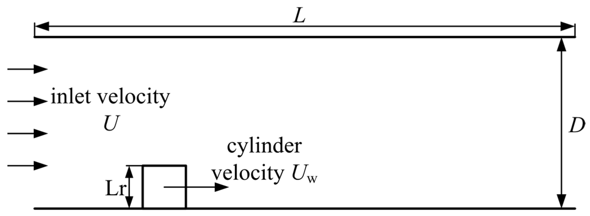
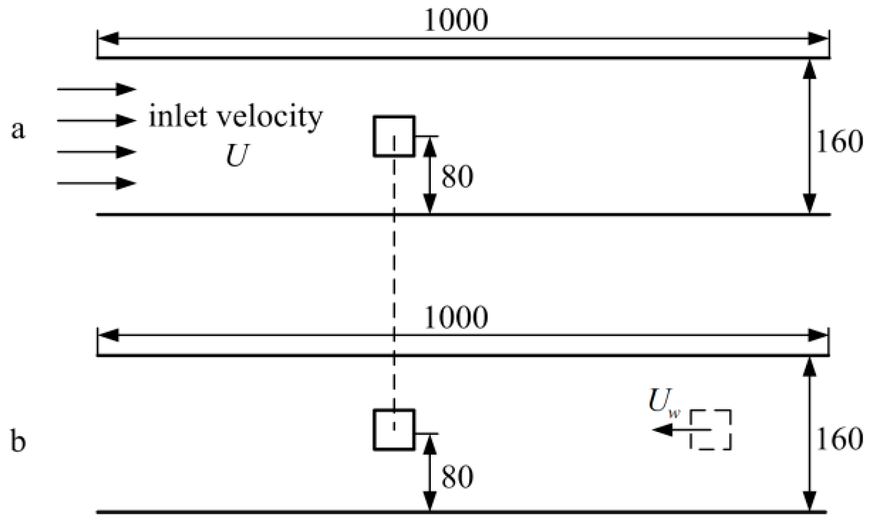
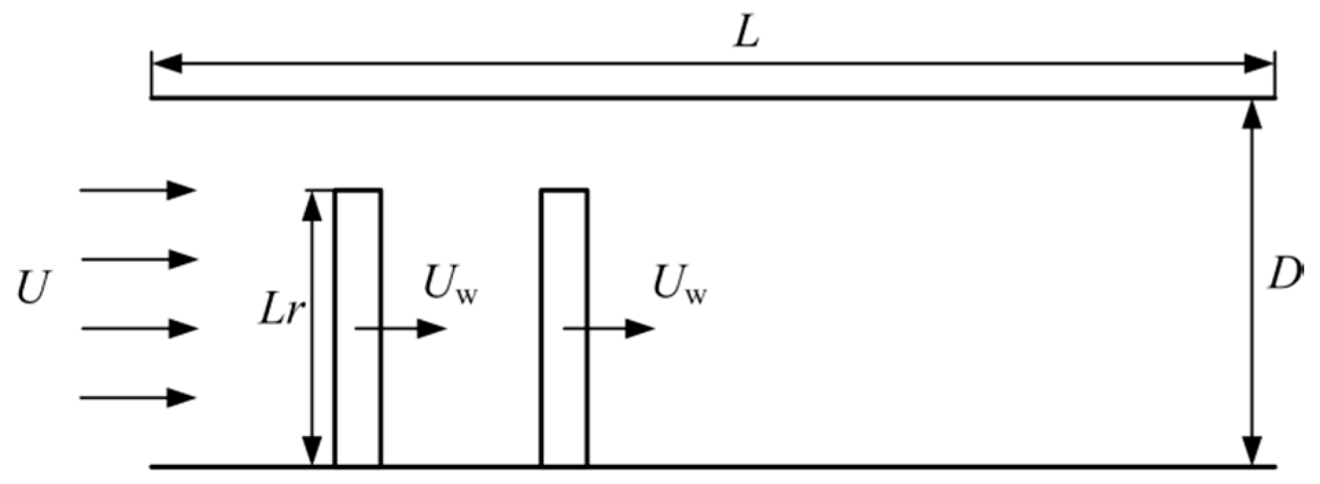
2.1. Physical Model

In the design and manufacture of heat exchange equipment, plug-in technology is a simple and effective way to strengthen heat exchange, and its essence is to enhance fluid turbulence. However, it is possible to form a reflow area in the rear of the static spoiler, and that can hinder convection heat transfer. Meanwhile, the thickness of boundary layer is an important factor that affects the heat transfer efficiency. Convection heat transfer is weak in the boundary layer because of the low velocity. Therefore, this paper hopes to drive the spoiler movement mechanically to destroy the reflow area and thin boundary layer. As shown in Figure 1, a square cylinder moves from left to right along the lower wall.

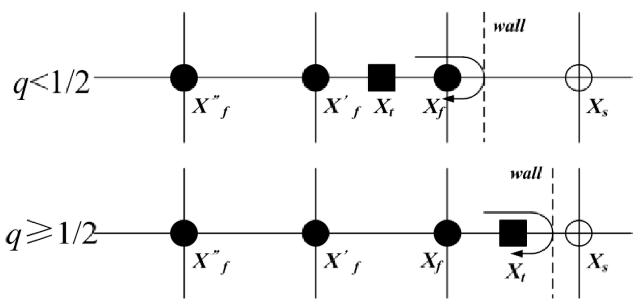
2.2. Lattice Boltzmann Method

The lattice Boltzmann method is based on kinetic theory. And the fundamental principle of LBM is using distribution functions f ( x , t ) to simulate the fluid flow at the mesoscopic scale. The distribution function f ( x , t ) represents the probability of the particles at position x and at time t moving with a velocity ei during the interval time Δt along each lattice line (i.e., direction i). The lattice Boltzmann equation (LBE) incorporating the single relaxation BGK approximation is given by Qian [23]:
f i ( x + e i Δ t , t + Δ t ) f i ( x , t ) = ω [ f i e q ( x , t ) f i ( x , t ) ]
where ω = 1 / τ denotes the relaxation factor, c s = c / 3 is the speed of sound, and c = Δ x / Δ t . The kinematic viscosity υ is given by the relaxation factor υ = ( 2 / ω 1 ) Δ x c / 6 . Aditionally, f i e q ( x , t ) is the equilibrium distribution, and is given by:
f i e q ( x , t ) = w i ρ [ 1 + e i u c s 2 + ( e i u ) 2 2 c s 4 u 2 2 c s 2 ]
For the D2Q9 model, the weightings in Equation (2) are assigned as follows: w i = 4 / 9 for e i = 0 , w i = 1 / 9 for e i = 1 , and w i = 1 / 36 for e i = 2 .
The density ρ and momentum ρu of fluid are obtained:
ρ = i f i , ρ u = i e i f i
In the problem of simulating the curved boundary, the solid boundary surface is either located on the solid node ( x s ) or on the middle between solid and fluid nodes ( x s and x f ). As shown in Figure 2, a parameter q can be used to describe the fraction of the link located in the fluid region, and can be defined as:
q = | x f x w | / | x f x s | = | x f x w | / Δ x
when 0 ≤ q ≤ 1.
For a rigid wall with no-slip condition, the bounce-back (BB) scheme is the most easily implemented boundary condition. Therefore, it is widely used in LBM simulations. The particle moves from flow to surface with velocity c i , and then reverses from the surface to flow with c i = c i at the solid surface, that is, the BB scheme.
For treating curved boundaries, Bouzidi [24] proposed a scheme by combining the BB scheme with an interpolation approach. By applying quadratic interpolation, the model takes the following form:
f i ( x f , t ) = { q ( 1 + 2 q ) f i ( x f + e i Δ t , t ) + ( 1 4 q 2 ) f i ( x f , t ) q ( 1 2 q ) f i ( x f e i Δ t , t ) , q < 1 / 2 1 q ( 2 q 1 ) f i ( x f + e i Δ t , t ) + 2 q 1 q f i ( x f e i Δ t , t ) 2 q 1 2 q + 1 f i ( x f 2 e i Δ t , t ) , q 1 / 2
For a moving wall treatment, a certain amount of momentum transfer between fluid and solid surfaces must be considered. Lallemand [25] applied Bouzidi’s model to treat the problem. So to reflect the fluid–solid interaction (i.e., the momentum transfer) at the boundary surface ( x s ), one additional term need be added to the distribution function. δ f i , the additional term, is given by:
δ f i = { 3 ω i ρ f e i u ω , 0 q < 1 / 2 3 q ( 2 q + 1 ) ω i ρ f e i u ω , 1 / 2 q 1
By applying the momentum exchange method [26], the drag and lift forces that are imposed by the fluid on the solid body can be determined by the formula:
F = x b i = 1 8 e i [ f i ( x b , t ) + f i ¯ ( x b , t + δ t ) ]

3. Results and Discussion

3.1. Model Validation

In order to validate the feasibility of Bouzidi’s interpolation-based model in dealing with a moving boundary, the verification simulations considering two cases of channel flow (i.e., a stationary square cylinder positioned in the channel and a square cylinder moving in the channel) are performed. As shown in Figure 3, a 1000 × 160 lattice structure is chosen for computation, and the square cylinder on the axis of the channel is assumed to have a side length of 20 lattice units (this article will always use lattice units). In this model, each lattice spacing corresponds to 1 mm, and each time step corresponds to 0.165 s. At the upper and lower walls, a no-slip boundary condition is imposed. In Figure 3a, square cylinder is stationary and inlet velocity U = 0.1 , and in Figure 3b, square cylinder velocity U w = 0.1 and inlet velocity U = 0 .
The numerical results of the moving boundary treatment in the two cases are compared in Figure 4, which show the distribution of the X-direction velocity component (U) on longitudinal section and the Y-direction velocity component (V) on cross section containing the center of the square cylinder. To make the comparison results more clearly and comparable, instead of the actual velocity, the relative velocity of the fluid, relative to the square, is used to denote the flow of the fluid. In Figure 3, it is obvious that the numerical results of both U and V are in excellent agreement except for the results of V on the longitudinal section. In addition, the order of magnitude of V on longitudinal section is so small (i.e., 10−13) that the slight volatility will make no difference. It can be concluded that, although physical models of the two cases are different, the numerical results of the two direction velocities on both sections are consistent, respectively.
In this simulation, the lift coefficient C l and the drag coefficient C d are two important dimensionless parameters for results validation, which are given by [22]:
C l = F l 1 / 2 ρ D U 0 2
C d = F d 1 / 2 ρ D U 0 2
The lift coefficient C l is constant equal to 0, for the square cylinder at the middle of the channel throughout the entire simulation. The comparison result of the drag coefficient C d is shown in Figure 5. In general, the results of the two cases show a good agreement.

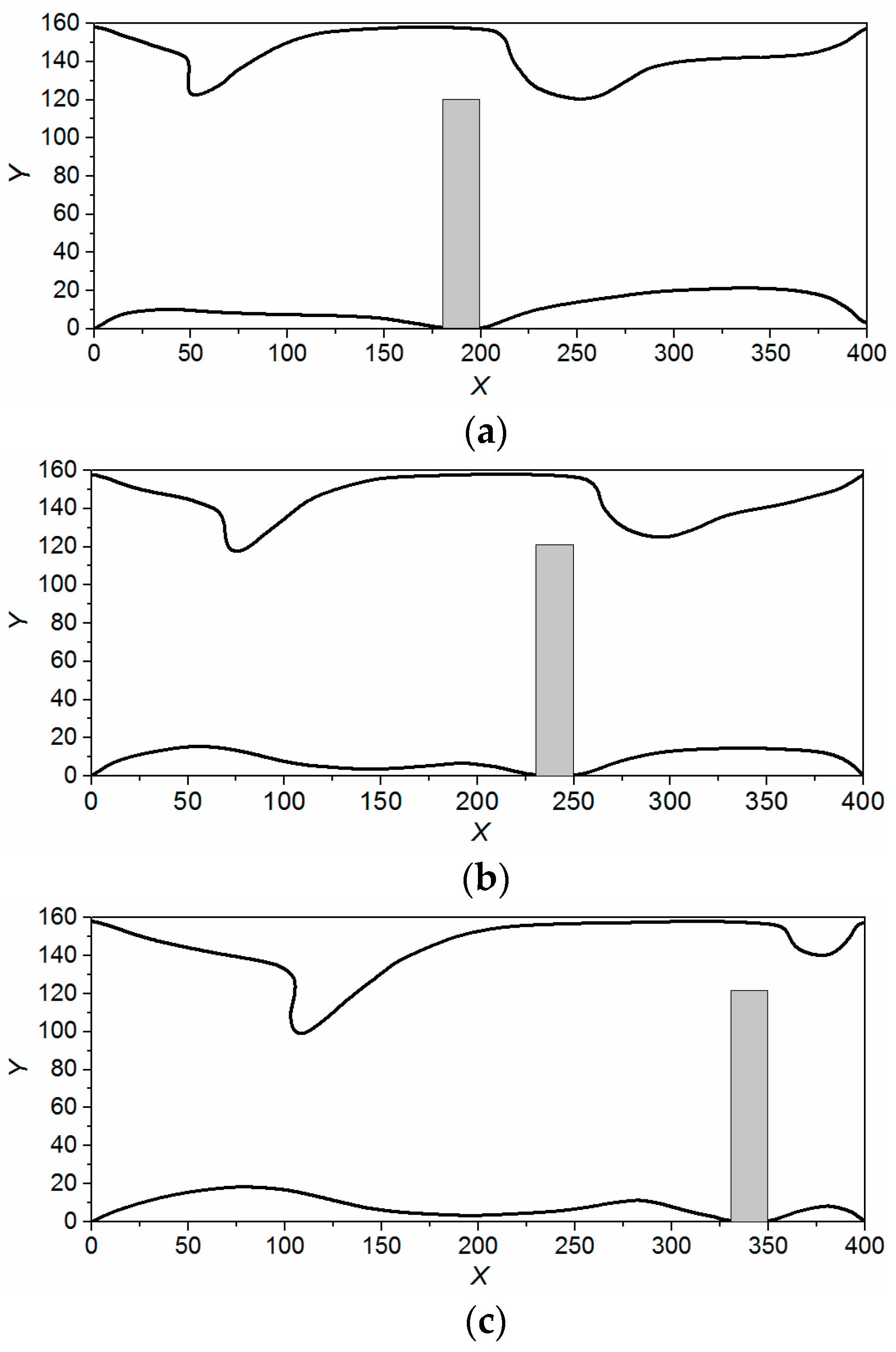
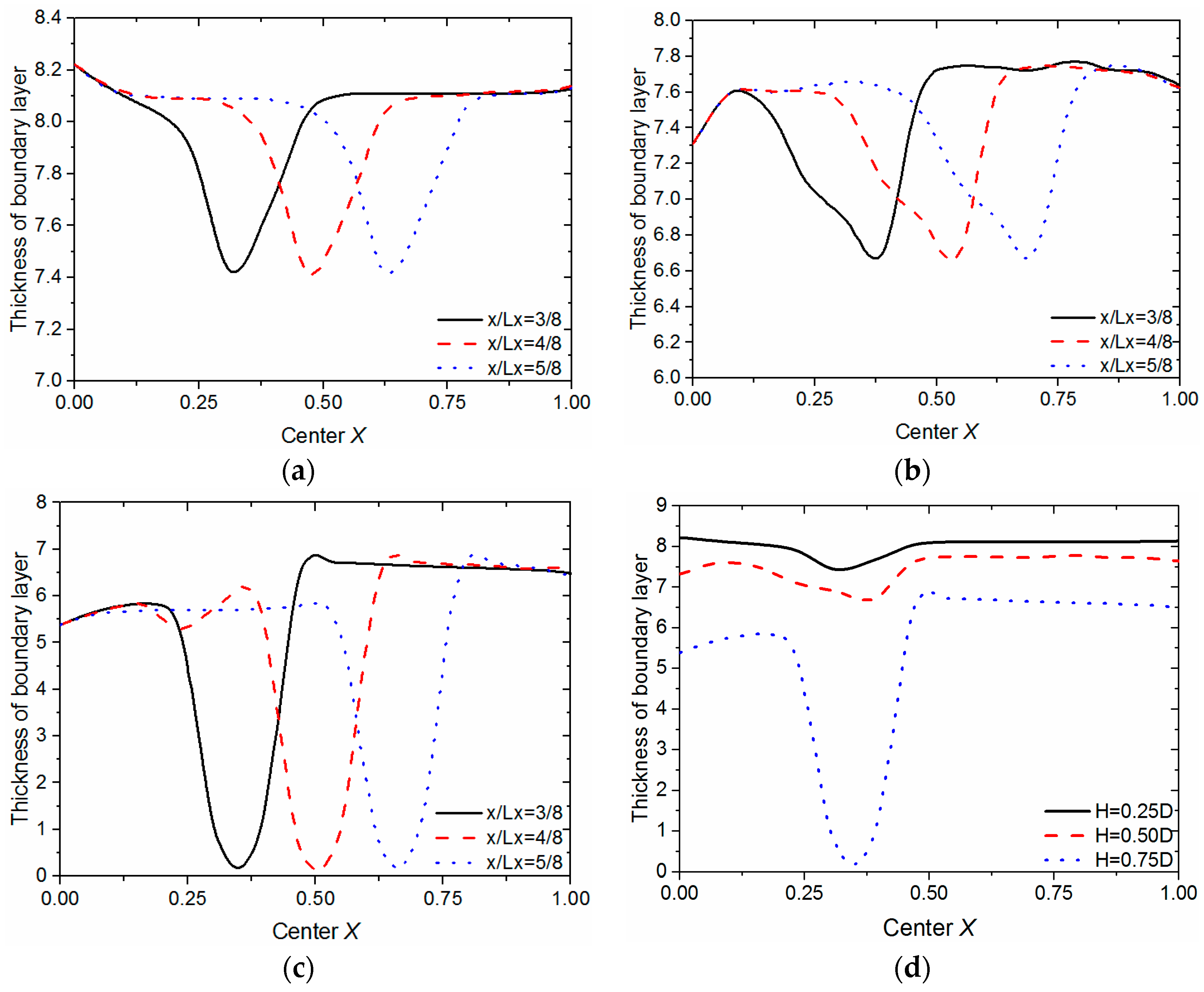
3.2. Effect of Square Cylinder with Different Height on Boundary Layer

When the square cylinder is placed in the flow field, the velocity of the flow field changes significantly, which causes the thickness of the boundary layer to change. As shown in Figure 6, the center line of the square cylinder with a height of 0.75D is set at 100 lattices in the calculation region of 400 × 160, which is proven to be suitable after grid-independence tests with 380 × 152, 400 × 600, 420 × 168, and the inlet velocity of the flow field is set to 0.05 lattice units. At the upper and lower walls, no-slip boundary condition is imposed. In this model, each lattice corresponds to 2.5 mm, and each time step corresponds to 4.95 s.
It can be seen that the velocity is faster in the area above the square cylinder, and is the smallest in the front and rear regions of the square cylinder, especially in the rear of the square column, which will cause the heat transfer capacity to deteriorate. Moreover, as shown in Figure 6b, under the same conditions, a square cylinder moves from left to right along the lower wall. When the square cylinder starts to move, the velocity distribution changes drastically in the flow field. Figure 6b shows that the square cylinder moves to 300 lattices. A huge vortex is formed in the area where the square cylinder passes, resulting in dramatic change in the flow field and an effective reduction of the boundary layer.
Figure 7a is about Re varies with Y-axis on different sections when the square cylinder is stationary. When x/Lx = 0.25, the fluid flows only from the upper side of the square cylinder, and the Reynolds number has the maximum value. When x/Lx = 0.50, Re has two peaks: the first peak is near the ordinate of 20. This is related to the surrounding vortex, and it will not improve the heat transfer efficiency; The second peak is near the ordinate of 120. Because the flow cross-sectional area decreases, the flow rate increases, resulting in the upper wall boundary layer thinning. When x/Lx = 0.75, the flow field tends to be stable. Figure 7b is about Re varies with Y-axis on different sections when the square cylinder moves to 300 lattices. Compared with the flow field of stationary pin fin, the magnitude of Re is basically the same. However, As the square cylinder moves, Re changes faster in the area near the solid walls, so the fluid velocity increases to the main velocity rapidly. This also verifies that the boundary layer is thinner in Figure 6b. Therefore, by reducing the boundary layer and eliminating the vortex behind the cylinder to improve the heat transfer efficiency is the basic starting point in this section.
In this section, the effect of square cylinder moving from left to right along the lower wall is studied. As shown in Figure 8 below, the computational domain is mapped using a 400 × 160 mesh, the height of the square cylinder is 0.75D (D is the channel diameter). The inlet velocity of the fluid U and square cylinder’s movement velocity U w are fixed at 0.05 and 0.1. Figure 8 shows the reconstruction of the boundary layer of the fluid in the process of a square cylinder moving from left to right along the channel. It is clear that as the square cylinder comes close and goes away, the boundary layer is destroyed, and then returns to its previous state, respectively. The boundary layer of the front and rear of the cylinder become obviously thinner through the movement.
In order to explore the effect of different height of the moving cylinder on the flow field, the height of the square cylinder is varied from 0.25D to 0.75D in increments of 0.25D. In Figure 9, X-direction indicates the ratio between the distance (x) from the inlet of the channel and the length of that, and Y-direction indicates thickness of the boundary layer. Figure 9a–c shows, as the square cylinder with different heights H (0.25D, 0.5D, 0.75D) moves to different locations (x/Lx = 3/8, 4/8, 5/8), the thickness of the boundary layer along the channel varies with that. It is obvious that the boundary layer in the location where the square cylinder moves to is the thinnest, and with the square cylinder going away, the boundary layer becomes gradually thicker until it returns to the original state it was. In Figure 9d, the results of that three square cylinders with different height move to the same location (x/Lx = 3/8) are compared. The conclusion can be drawn that the thickness of the boundary layer decreases with the square cylinder’s height increasing.

3.3. Double Cylinders Model

From the above simulation, the boundary layer will be reconstructed after the cylinder passes by. So another cylinder is added to destroy the boundary layer again, which can both lengthen the domain with thinner boundary layer and strengthen the mixture and disturbance of the flow to enhance the heat transfer further. As shown in Figure 10, the computational domain is mapped using a 1000 × 160 mesh, the side length of the cylinders is 20, the height of both cylinders is 0.75D. As well, the velocity of the liquid in the channel is U = 0.05 . Two cylinders with a certain distance move at the same velocity of U w = 2 U to destroy the boundary layer.
Figure 11 shows the thickness of boundary layer changing with the non-dimensional time. With the movement of the cylinders from left to right, the thickness of the boundary layer changes with the increase of value n along X axis, which are compared with the thickness of boundary layer of Poiseuille flow. It is obvious that, in most part of the channel, the boundary layer of double cylinders model is much thinner than that of Poiseuille flow. However, at the domain behind the cylinders, the thickness of boundary layer become thicker, which increases the thermal resistance to some extent, regardless of increasing the disturbance. Taken together, the effect of the double cylinders on thinning boundary layer and enhancing heat transfer is highlighted.
The distance of the double cylinders has an obvious effect on the thickness of boundary layer. In some cases, it did not reduce the thickness of boundary layer effectively. Therefore, the optimized distance of the double cylinders is needed for design by simulation. The thickness curves of boundary layer with the different interval distance of the double cylinders at the same time and the same Re number are shown in Figure 12. At the domain from 400 to 500 in the X coordinate, the thickness of the boundary layer may has crests or troughs with different value of interval distance of the double cylinders. There is an optimal interval distance in the domain of 60~180. The effect of the interval distance is obvious from 400 to 500 in the X coordinate. The Figure 13 shows the thickness of the boundary layer with different interval distance of the double cylinders at x = 450. Thus, the optimal interval distance of the double cylinders is between 90 and 140.

4. Conclusions

In this paper, we have characterized the moving boundary with the lattice Boltzmann method. In order to provide the basis for the realization of the heat exchanger’s performance optimization and solid attachments flowing out of the heat exchanger with the water, the boundary layer reconstruction model is established. According to the simulation results, conclusions can be drawn as followed.
(1)
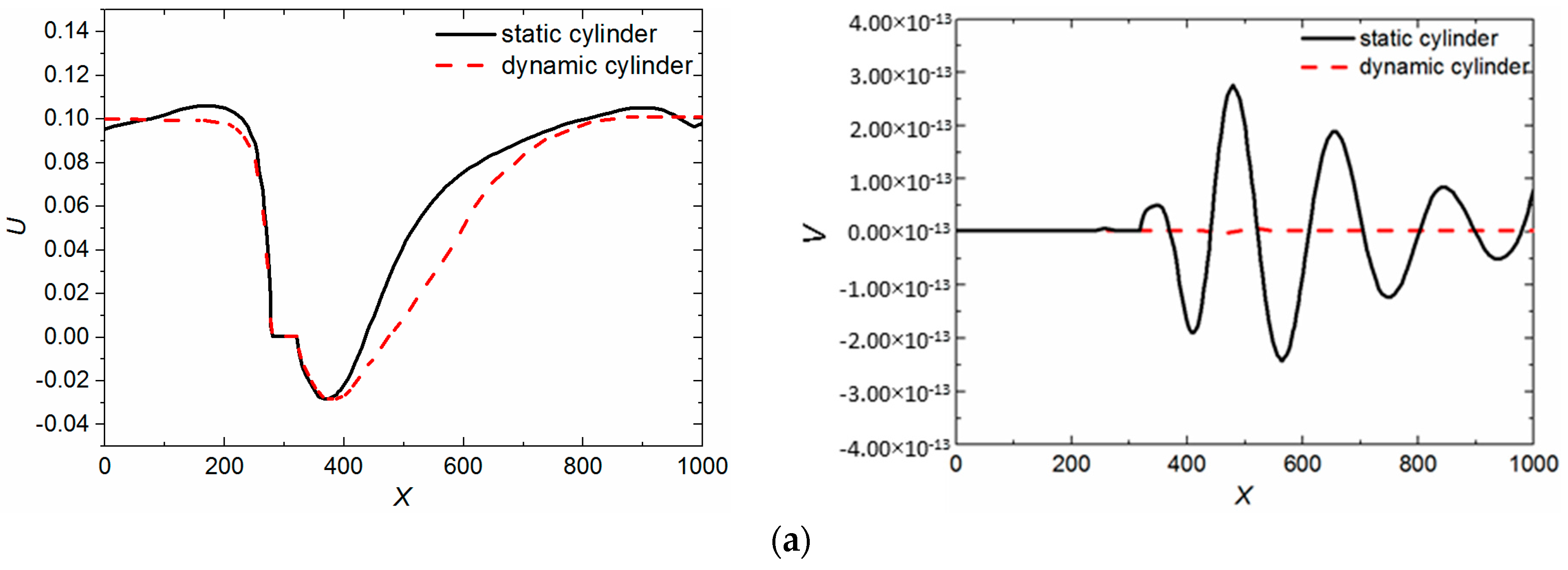
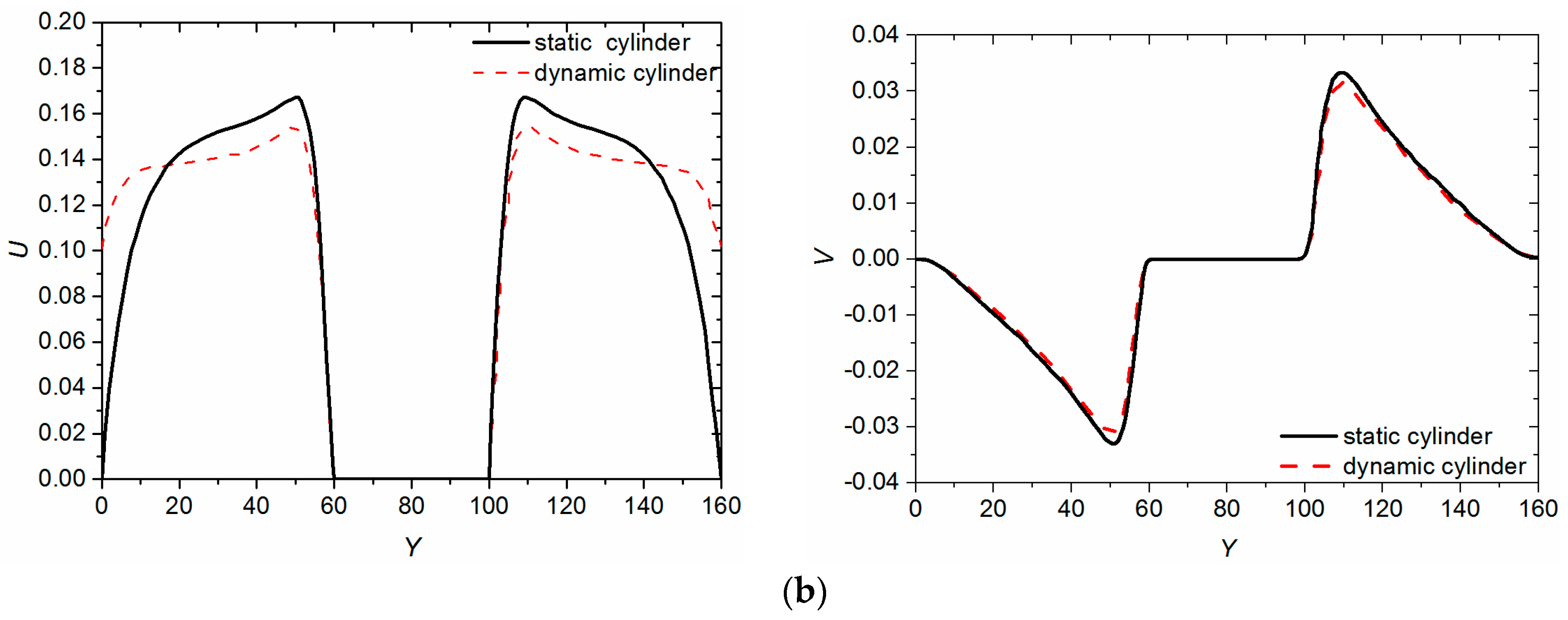
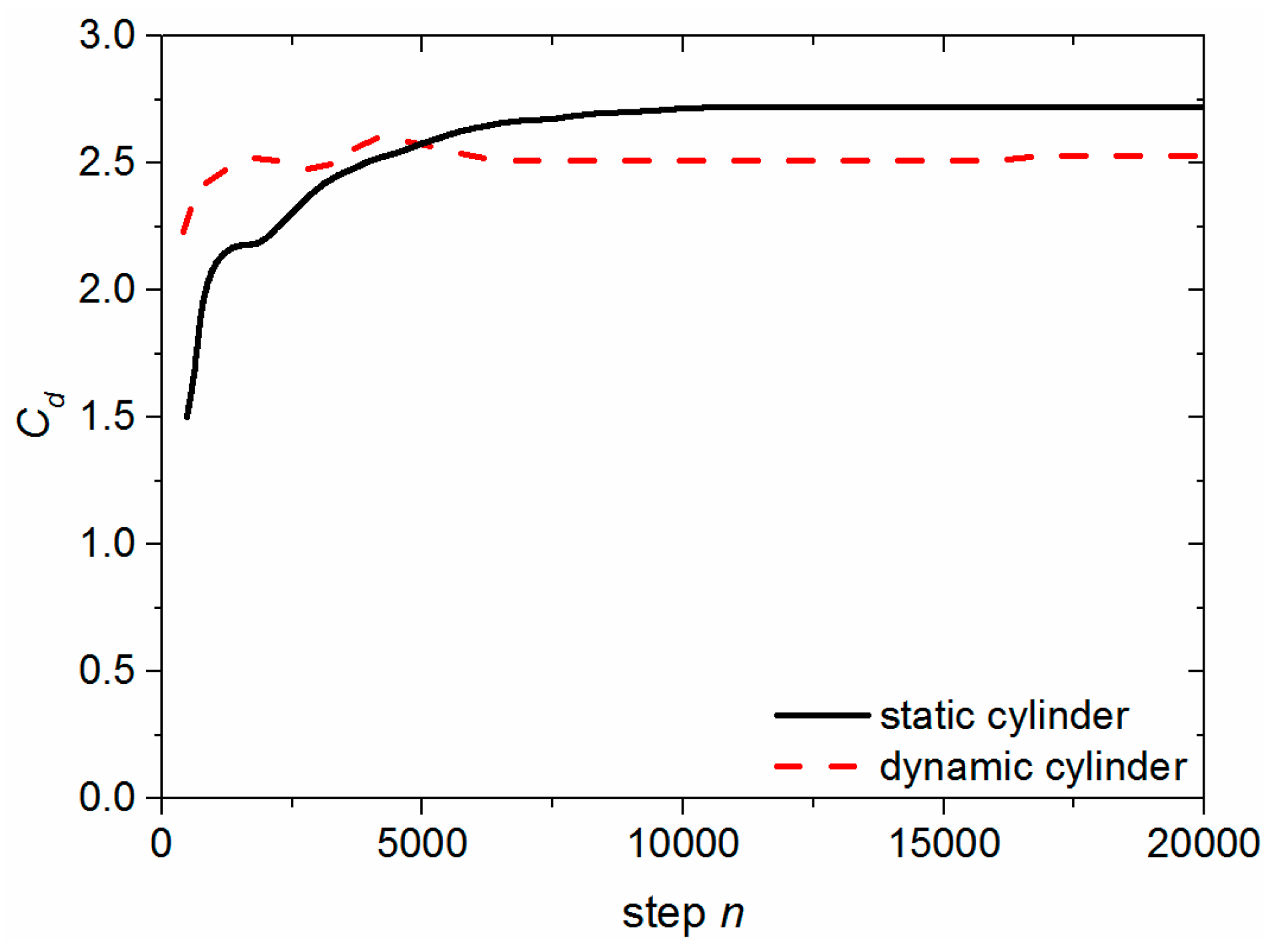
By comparing the changes of the X-direction velocity component (U) and the Y-direction velocity component (V) and lift and drag in the center of the square cylinder, the conclusion that lattice Boltzmann method has the feasibility and superiority in dealing with moving boundary is obtained.
(2)
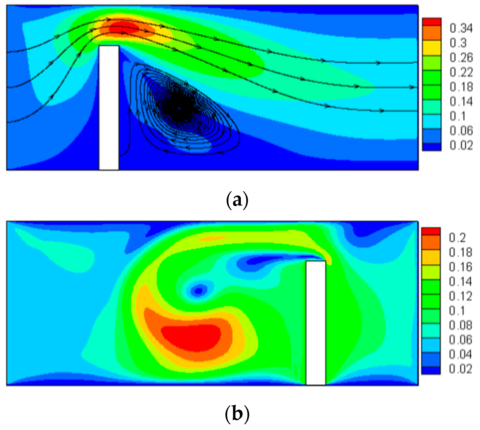
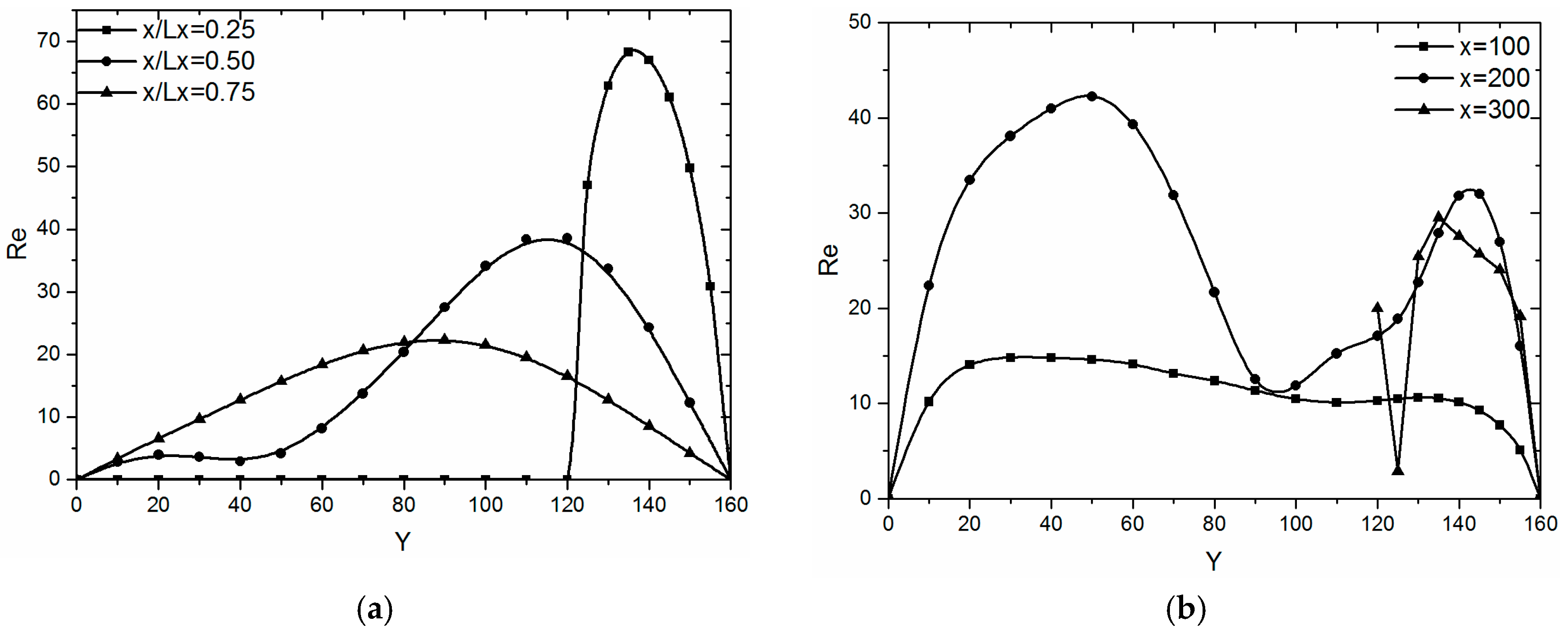
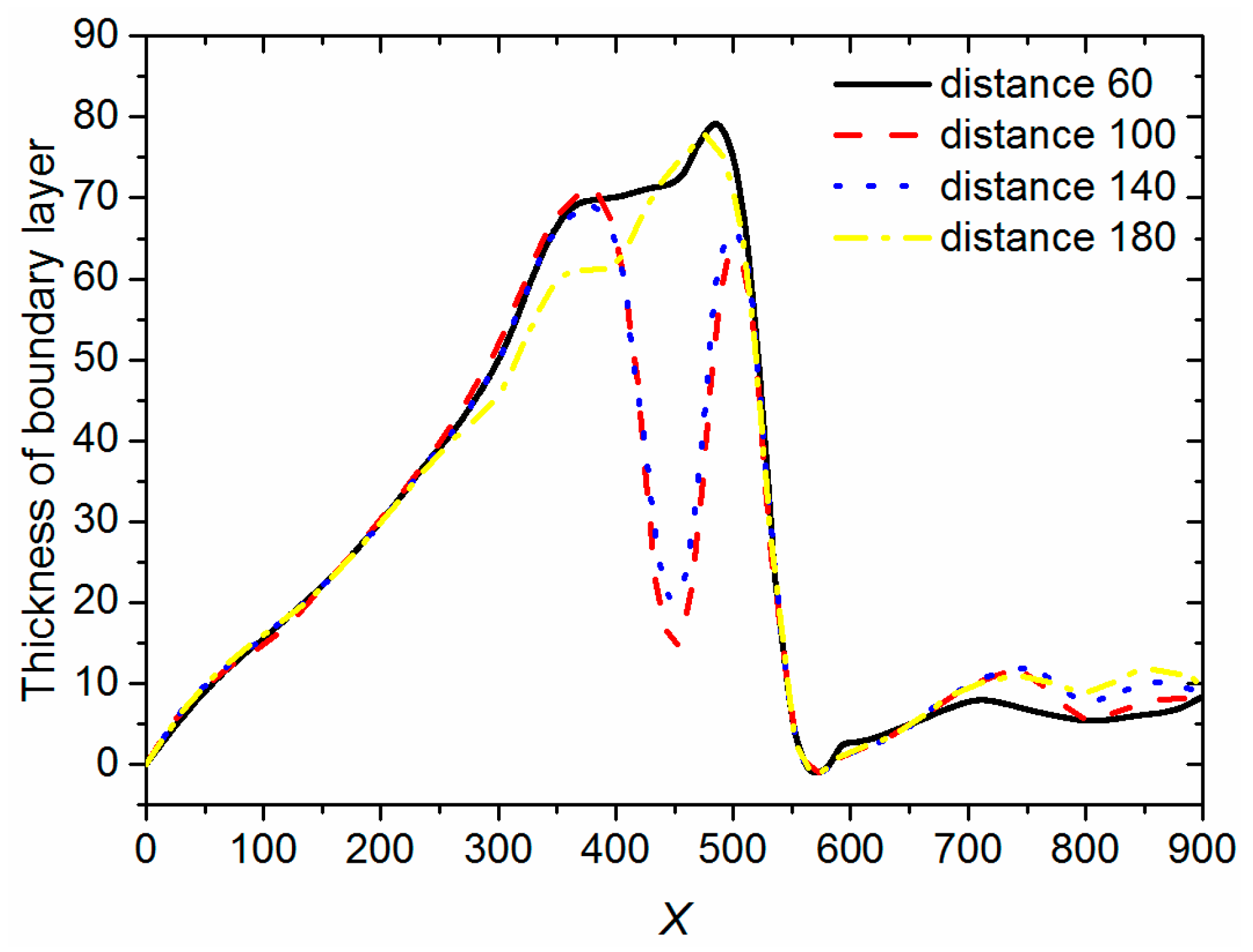
The boundary layer reconstruction model has been established. It is found that when the square cylinder is present, the fluid boundary layer will be destroyed to enhance the total heat transfer coefficient, which makes the optimization of the heat exchanger possible. At the same time, the thickness of the boundary layer increases as the height of the square cylinder decreases.
(3)
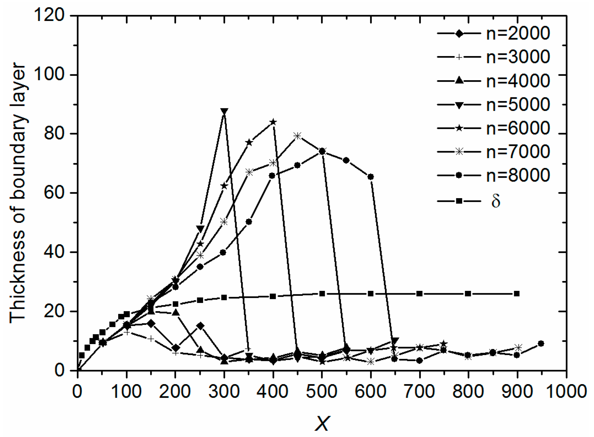
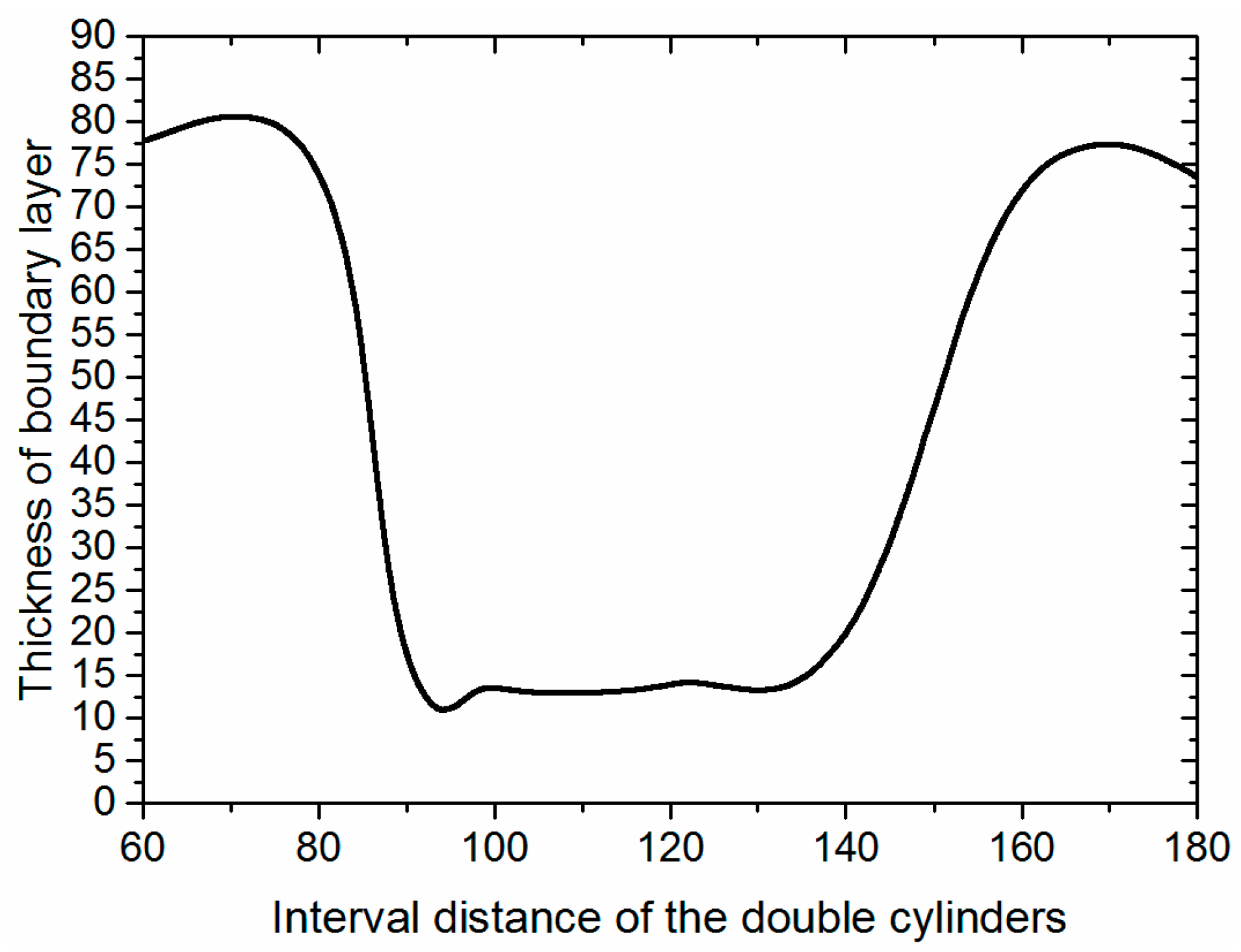
As the square cylinder passes by, the boundary layer away from the square cylinder will gradually thicken and be reconstructed. Double cylinders are effective to make the boundary layer continuously thin, and there is an optimum interval distance of the cylinders.

Acknowledgements

This work was supported by the National Natural Science Foundation of china under Grant No. 51376164 and Natural Science Foundation of Shandong Province under Grant No. ZR2013EEQ034. In addition, this is an extension of the work presented at ICEER2017 and published Energy Procedia.

Author Contributions

Yan Li, Chuan Li and Cong Liu designed the numerical simulation and analyzed the data; Yajie Wu, Han Yuan and Ning Mei revised the manuscript.

Conflicts of Interest

The authors declare no conflict of interest.

References

  1. Shirvan, K.M.; Mamourian, M.; Mirzakhanlari, S.; Ellahi, R.; Vafai, K. Numerical investigation and sensitivity analysis of effective parameters on combined heat transfer performance in a porous solar cavity receiver by response surface methodology. Int. J. Heat Mass Tranf. 2017, 105, 811–825. [Google Scholar] [CrossRef]
  2. Shirvan, K.M.; Ellahi, R.; Mirzakhanlari, S.; Mamourian, M. Enhancement of heat transfer and heat exchanger effectiveness in a double pipe heat exchanger filled with porpous media: Numerical simulation and sensitivity analysis of turbulent fluid flow. Appl. Therm. Eng. 2016, 109, 761–774. [Google Scholar] [CrossRef]
  3. Sheikholesmi, M.; Zia, Z.Q.M.; Ellahi, R. Influence of induced magnetic field on free convection of nanofluid considering Koo-Kleinstreuer-Li(KKL) correlation. Appl. Sci. 2016, 6, 324. [Google Scholar] [CrossRef]
  4. Shirvan, K.M.; Mamourian, M.; Ellahi, R. Numerical investigation and optimization of mixed convection in ventilated square cavity filled with nanofluid of different Inlet and outlet port. Int. J. Numer. Methods Heat Fluid Flow 2017, 27, 2053–2069. [Google Scholar] [CrossRef]
  5. Kandelousi, M.S.; Ellahi, R. Simulation of ferrofluid flow for magnetic drug targeting using the lattice Boltzmann method. Zeitschrift für Naturforschung A 2015, 70, 115–124. [Google Scholar] [CrossRef]
  6. Shirvan, K.M.; Mamourian, M.; Mirzakhanlari, S.; Ellahi, R. Numerical investigation of heat exchanger dffectiveness in a double pipe heat exchanger filled with nanofluid: A sensitivity analysis by response surface methodology. Powder Technol. 2017, 313, 99–111. [Google Scholar] [CrossRef]
  7. Pasquetti, R.; Bwemba, R.; Cousin, L. A pseudo-penalization method for high Reynoles number unsteady flows. Appl. Numer. Math. 2008, 58, 946–954. [Google Scholar] [CrossRef]
  8. Kim, D.K. Thermal optimization of branched-fin heat sinks subject to a parallel flow. Int. J. Heat Mass Tranf. 2014, 77, 278–287. [Google Scholar] [CrossRef]
  9. Wang, Y.; Yan, Z.; Wang, H. Numerical simulation of low-Reynolds number flows part two tandem cylinders of different diameters. Water Sci. Eng. 2013, 6, 433–445. [Google Scholar]
  10. Shirvan, K.M.; Mamourian, M.; Mirzakhanlari, S.; Rahimi, A.B.; Ellahi, R. Numerical study of surface radiation and combined natural convection heat transfer in a solar cavity receiver. Int. J. Numer. Methods Heat Fluid Flow 2017, 27, 2385–2399. [Google Scholar] [CrossRef]
  11. Saha, A.K.; Acharya, S. Parametric study of unsteady flow and heat transfer in a pin-fin heat exchanger. Int. J. Heat Mass Tranf. 2003, 46, 3815–3830. [Google Scholar] [CrossRef]
  12. Sharman, B.; Lien, F.S.; Davidson, L.; Norberg, C. Numerical predictions of low Reynolds number flows over two tandem circular cylinders. Int. J. Numer. Methods Fluids 2005, 47, 423–447. [Google Scholar] [CrossRef]
  13. Rashidi, S.; Esfahani, J.A.; Ellahi, R. Convective heat transfer and particle motion in an obstructed duct with two side by side obstacles by means of DPM model. Appl. Sci. 2017, 7, 431. [Google Scholar] [CrossRef]
  14. Lu, J.; Han, H.; Shi, B. A numerical study of fluid flow passes two heated/cooled square cylinders in a tandem arrangement via lattice Boltzmann method. Int. J. Heat Mass Tranf. 2012, 55, 3909–3920. [Google Scholar] [CrossRef]
  15. Kotcioglu, I.; Caliskan, S.; Baskaya, S. Experimental study on the heat transfer and pressure drop of a cross flow heat exchanger with different pin-fin arrays. Heat Mass Transf. 2011, 47, 1133–1142. [Google Scholar] [CrossRef]
  16. Shi, Z.; Dong, T. Entropy generation and optimization of laminar convective heat transfer and fluid flow in a microchannel with staggered arrays of pin fin structure with tip clearance. Energy Convers. Manag. 2015, 94, 493–504. [Google Scholar] [CrossRef]
  17. Chang, S.; Chen, C.; Cheng, S. Analysis of convective heat transfer improved impeller stirred tanks by the lattice Boltzmann method. Int. J. Heat Mass Tranf. 2015, 87, 568–575. [Google Scholar] [CrossRef]
  18. Agrawal, S.; Terrence, W.S.; North, M.; Bissell, D.; Cui, T. Heat transfer augmentation of a channel flow by active agitation and surface mounted cylindrical pin fins. Int. J. Heat Mass Tranf. 2015, 87, 557–567. [Google Scholar] [CrossRef]
  19. Yoon, H.S.; Chun, H.H.; Kim, J.H.; RyongPark, I.L. Flow characteristics of two rotating side-by-side circular cylinder. Comput. Fluids 2009, 38, 466–474. [Google Scholar] [CrossRef]
  20. Yan, Y.Y.; Zu, Y.Q. Numerical simulation of heat transfer and fluid flow past a rotating isothermal cylinder—A LBM approach. Int. J. Heat Mass Tranf. 2008, 51, 2519–2536. [Google Scholar] [CrossRef]
  21. Bhatnagar, P.L.; Gross, E.P.; Krook, M. A model for collision processes in gases. I. small amplitude processes in charged and neutral one-component systems. Phys. Rev. 1954, 94, 511–524. [Google Scholar] [CrossRef]
  22. He, X.Y.; Luo, L.S. Lattice Boltzmann model for the incompressible Navier-Stokes equation. J. Stat. Phys. 1997, 88, 927–944. [Google Scholar] [CrossRef]
  23. Qian, Y.H.; Dhumieres, D.; Lallemand, P. Lattice BGK models for Navier-Stokes equation. Europhys. Lett. 1992, 17, 479. [Google Scholar] [CrossRef]
  24. Bouzidi, M.; Firdaouss, M.; Lallemand, P. Momentum transfer of a Boltzmann-lattice fluid with boundaries. Phys. Fluids 2001, 13, 3452–3459. [Google Scholar] [CrossRef]
  25. Lallemand, P.; Luo, L.S. Lattice Boltzmann method for moving boundaries. J. Comput. Phys. 2003, 184, 406–421. [Google Scholar] [CrossRef]
  26. Ladd, A. Numerical simulations of particulate suspensions via a discretized Boltzmann equation Part 2. Numerical results. J. Fluid Mech. 1999, 271, 311–339. [Google Scholar] [CrossRef]
Figure 1. Physical model of moving square cylinder.
Energies 10 02074 g001
Figure 2. 1D projection of curved boundary based on regular grid (arrows indicate the direction of the fluid particle movement).
Energies 10 02074 g002
Figure 3. Physical model of square cylinder around the flow. (a) Inlet velocity U = 0.1 , square cylinder’s velocity U w = 0 and (b) Inlet velocity U = 0 , square cylinder’s velocity U w = 0.1 .
Energies 10 02074 g003
Figure 4. Comparison of numerical results of U and V on cross section and longitudinal section. (a) Comparison of U and V on longitudinal section and (b) Comparison of U and V on cross section.
Energies 10 02074 g004aEnergies 10 02074 g004b
Figure 5. Comparison results of drag coefficient C d .
Energies 10 02074 g005
Figure 6. The distribution of velocity with a pin fin. (a) Static pin fin, (b) Moving pin fin.
Energies 10 02074 g006
Figure 7. Re varies with Y-axis on different sections. (a) Static pin fin (x/Lx = 0.25); (b) Moving pin fin (x/Lx = 0.75).
Energies 10 02074 g007
Figure 8. Contour line of the boundary layer in the flow field at different n (n is the simulation steps). (a) n = 900; (b) n = 1400; (c) n = 2400.
Energies 10 02074 g008
Figure 9. Changes of the thickness of the boundary layer in different locations (x/Lx = 3/8, 4/8, 5/8). (a) H = 0.25D; (b) H = 0.50D; (c) H = 0.75D; (d) x/Lx = 3/8.
Energies 10 02074 g009
Figure 10. Physical model of double cylinders.
Energies 10 02074 g010
Figure 11. Thickness of the boundary layer of double cylinders at different n.
Energies 10 02074 g011
Figure 12. The thickness of the boundary layer with different interval distance of the double cylinders (interval distance of the double cylinders is 60, 100, 140, 180).
Energies 10 02074 g012
Figure 13. The thickness of the boundary layer with different interval distance of the double cylinders at x = 450 in Figure 10.
Energies 10 02074 g013

