Evaluation of Comfort Level and Harvested Energy in the Vehicle Using Controlled Damping

Abstract

Shock absorbers allow the damping of suspension vibrations, by dissipating kinetic energy. This energy theoretically can be harvested; however, practical solutions are not easily obtainable. This paper is dedicated to analyzing and evaluating the vibration energy in a vehicle’s suspension that is generated by road excitations. Also, it estimates the possible amount of harvested energy required to diminish accelerations of the vehicle body, the driver, or the passenger center of mass. The control of damper is realized by optimizing the best damping coefficient for different road roughness. Analytical results, obtained from the proposed dynamic model of the car, were compared with experimental data, showing a good coherence between them. These results allow us to evaluate the amount of energy circulating within shock absorbers and give information about the amount of the possible harvested energy. There is a very good relationship between energy needed for control and gained energy.

1. Introduction

Energy harvesting and vibration control from large amplitude and low frequency vibrations is a promising research area [1,2,3,4,5,6,7,8,9,10,11]. Electromagnetic (EM) transducers are widely used for this purpose. Transducers can be coupled to a permanent-magnet synchronous machine [1], or linear motion EM devices [2,10], which can be used for both vibration damping and energy harvesting. An energy harvesting-enabled tuned mass-damper-inerter system comprises a mass, grounded via an electromagnetic motor (energy harvester)-inerter layout [8]. An electromagnetic resonant shunt tuned mass-damper-inerter was proposed by Luo et al. [9]. This control device can help in minimizing structure damage and simultaneously harvest energy under random wind excitation [9]. Vibration control, together with energy harvesting, possibly could be realized, by using a vibration absorber, supplemented with a piezoelectric stack [4,7]. However, such vibration control systems can be applied only to high vibration frequencies, since the output power at low frequencies becomes very small. Moreover, the piezoelectric energy harvester maximum generated power is in the range of milliwatts [12,13].

A vehicle’s damping system control should comply with specific purposes, such as passenger riding comfort and the vehicle’s handling quality improvement [14,15,16,17]. A recent study demonstrated a significant enhancement in harvested power and the frequency bandwidth of a multimodal electromagnetic vibration energy harvester, consisting of arrays of coupled levitated magnets [18], when the device is excited beyond its critical Duffing amplitude [19]. The automobile shock absorber practically always works under random excitations [7], caused by the irregularity of road surface, and during acceleration or braking [20,21,22,23,24,25]. The intensity of these excitations is proportional to the vehicle speed. Different control techniques could be used for vibration control in a car. One amongst the most effective and low-cost systems is semi-active [3,26] with magnetorheological (MR) dampers [14,16,27]. Such systems are used to minimize the response to external disturbances, with a small amount of power, compared to active systems [28]. MR dampers are widely used in the automotive industry, train suspension systems, seismic protection and in cable-stayed bridges [29,30,31]. Semi-active vibration control systems could be composed of an MR damper and an electromagnetic vibration energy harvester. Harvested energy in such systems is used to power the MR damper. Another way to suppress the vibration and harvest the energy is to use acoustic–elastic material metastructure with piezo elements [32,33]. However, finding optimal parameters for such system control is complicated, because for vibration suppression and for energy harvesting performances, the parameters have to be tuned in opposite directions. Therefore, for such damping/harvesting systems, the quality of damping/harvesting is a compromise: when damping is improved, harvested energy is small, and vice versa.

The control of semi-active systems with MR dampers are often realized by controlling the viscosity of the magnetorheological fluid. However, using this control method, heat is generated in the inductor coil as well as energy dissipation from vibrations. The main problem of dampers of this type, is the excess heat, which decreases its working effectiveness. On the other hand, the damper works with only some limitations in time and coil current. Moreover, the fluid must be cooled and pumped over. Thus, such type of damper could not be used as an energy harvester.

In order to extract as much energy as possible from the energy harvester, it is necessarily to adopt proper AC/DC converter topologies and control techniques, such as those reported in [34,35,36,37]. In practice, joint mechanical and electrical optimization is necessary.

The new type of damper-energy harvester device, based on implementation of ferro-nanomagnetic fluid was presented in [14]; this particular fluid is used as: (i). ferromagnetic media; (ii). lubricant for bonding surfaces; and (iii). hydraulic fluid for vibration damping, as in classic shock absorbers in vehicles. To take full advantage of this device, a specific mathematical model is necessary to evaluate the generation of power from vibration and consequently to create the control system. Different mathematical models for similar devices have been proposed—from an individual MR damper model to models of the whole car body. Many authors are trying to optimize dampers using different control algorithms, models and controllers, such as: (i). semi-active damping force estimator [38]; (ii). sliding model controller [21]; (iii). skyhook, ground hook and hybrid systems [39]; (iv). 8 degrees of freedom (DOF)whole body vehicle model [23]; (v). non-parametric linearized data driven model [28]; (vi). skyhook controller in hardware-in-the-loop simulation [22]; (vii). hybrid control [40]; (viii). valve system optimization model [41]; (ix). vibration control method, used in earthquakes [11]; (x). variable damping coefficients observation by controlling the electrical load of the shock absorber [42]. The latter findings most relate to our research—we are trying to find optimized damping coefficient values, which will be realized using the real vibration control and harvesting system, proposed in [14]. In [42] authors presented variable damping coefficients. However, in this case, controllable electrical current was applied for damping control, thus, the damping coefficient was not changed according to vibration characteristics. Thus, it is not possible to change the moving regime without feedback. Moreover, there is no possibility of harvesting the energy and using it for damper control. In commercially available systems, three main places of the vehicle are usually damped: the tire, suspension, and seat. The mathematical models, mentioned above, do not evaluate all these parameters either. Additionally, our model evaluates another important shock absorber application possibilities—harvesting energy from vibrations. There are some problems in using shock absorbers as automobile energy harvesters: (i). vibrational energy systems may not achieve the entire frequency range needed for harvesting and (ii). optimizing energy harvesting and vibration damping are often competing goals [14].

In this context, the main aim of this research is to propose a new damping system control method, with optimized damping coefficients, of which values are related to road roughness and to evaluate this optimized control effect for the amount of generated energy. The paper presents a new damping system control method and the possibility to apply such a system for energy harvesting. Our control method, presented here, and device, proposed in [14], could be applied to the harvest of all types of vibration energy, including vibrations from earthquakes. However, at low frequency vibrations, which usually occur in buildings, the amount of harvested energy will be very low.

2. Materials and Methods

Experiments were performed by the car, Range Rover Evoque, on two roads—road no. 6 (coarsest) and road no. 3 (medium roughness)—with the driver, whose mass was 80 kg, but without passengers or baggage. Acceleration were measured by two accelerometers (damping coefficient 7500 Ns/m), placed in the car, Range Rover Evoque, as shown in Figure 1. The speed of the car was 60 kph. Measurements were performed using industrial equipment, piezoelectric accelerometers (603C01 from PCB Piezotronics, Depew, NY, USA), and a data acquisition device (NI 4431 from National Instruments, Austin, TX, USA). Data were collected using the National Instruments Software Package, LabView 2015. In order to compare experimental and analytical data, the damping force was calculated from an experimentally-observed suspension position:

$$F_{\exp }=h_{sF1}\cdot \dot{Z}+k_{sF}\cdot Z$$

(1)

The model was solved using MatLab version 2014b. The simulation took 1 min for each 1 s of real road. Equations were solved in Simulink, by means of the standard fourth order Runge–Kutta solver.

3. Mathematical Model

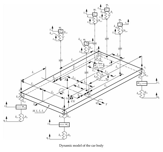
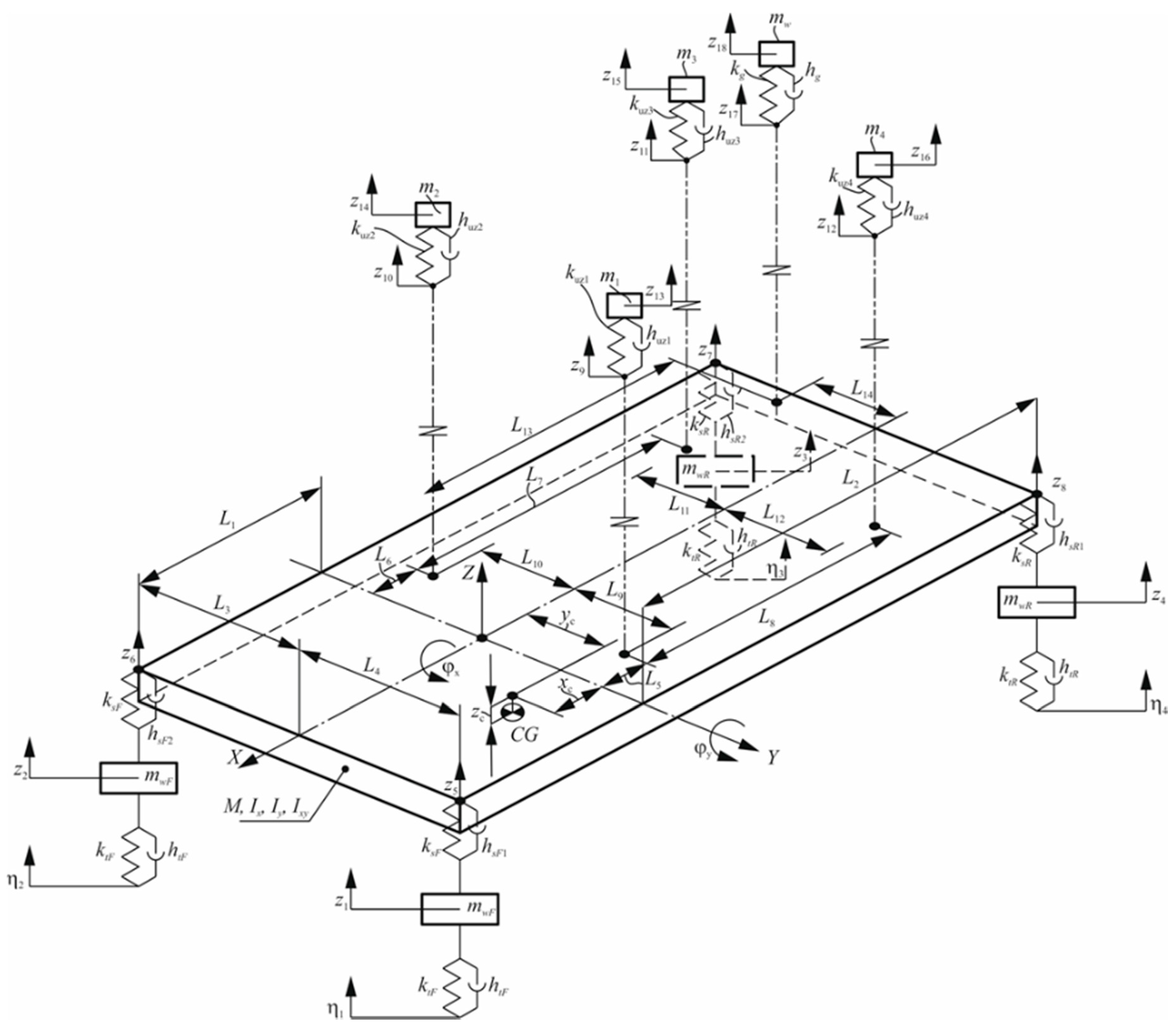
3.1. Dynamic Model of the Vehicle

The model of the car body included ten masses and two moments of inertia. Other masses and moments of the car are reduced by joining them with respect to the transfer ratio of the suspension levers. The model also included four passengers’ masses and the mass in the baggage box, as presented in Figure 2. The masses of the tires and the rims were included into suspension masses; they have independent coordinates.

In the proposed model, the car frame is regarded as a rigid body and is here named the system, as the stiffness of it is a few orders of magnitudes higher than the suspension stiffness. The movement of the system is described with the coordinate of the vertical axis, Z, and the rotation angles, φ_x and φ_y, about the axes, X and Y, respectively. The origin is considered to coincide with the stiffness center in the plane of the suspension springs of the upper point. In general, the center of gravity does not coincide with the center of stiffness. Coordinates of the center of gravity with respect to the center of stiffness are denoted as x_s, y_s and z_s.

In the model, the parameters of the car body were: the mass of the car (M), the moments of inertia about the respective axis (J_x and J_y), and the mixed moment (J_xy). Displacements in X and Y axes and rotations about the Z axis were ignored, because only the main affecting vibrations in the vertical direction to the human body were evaluated. The suspension was modelled with elastic damping elements. It was considered that the elastic stiffness of the elements was linear.

Stiffness coefficients of the front wheel suspension of individual elastic elements are denoted as k_sF. Stiffness coefficients of the rear wheel suspension of individual elastic elements are denoted as k_sR.

Suspension shock absorbers here were modelled as nonlinear damping elements. The damping coefficients, h_sF1, h_sF2, h_sR1, h_sR2, depended on the velocity of vertical wheel movement caused by the roughness of the road. Here, the presented model evaluates only vertical movements of wheels, represented by the coordinates, z₁, z₂, z₃, z₄. In the model, the weight of the hub was evaluated as the sum of the masses of the tire, rim, axle, bearing and support. Suspension parts, which were connected to the lower suspension spring points were added to the reduced wheel masses, as unsuspended masses (m_wF). It was assumed that the suspension mass (m_wF) and the rear mass (m_wR) were included in the front wheel mass. It was also assumed that the tire of the vehicle is modelled as a spring with a damper. The front wheel tire spring element coefficient of stiffness was marked as k_sF, for the rear wheel (k_sR). The coefficients of damping are marked h_sF and h_sR, respectively.

The driver, three passengers and load in the baggage box were modelled as masses, m₁, m₂, m₃, m₄, m_w, mounted on the stiffness elements, k_uz1, k_uz2, k_uz3, k_uz4 and k_g, with dampers, h_uz1, h_uz2, h_uz3, h_uz4 and h_g, respectively.

Stiffness elements were applied to the vehicle body by distances, L₁, ..., L₁₄. The dynamic system (the car) was excited kinematically along the coordinates, η₁, η₂, η₃, η₄. In this case, the principle of relativity to the car body admits that the car is staying immobile in the horizontal plan and the road is moving.

The status of the dynamic behavior of the vehicle was defined by twelve generalized coordinates—Z, φ_x, φ_y, z₁, z₂, z₃, z₄, z₁₃, z₁₄, z₁₅, z₁₆, z₁₈. For the purpose of better visualization and to build general equations, there were also some defined auxiliary coordinates: the shock absorbers’ points (z₅, z₆, z₇, z₈), the points of seat contact with the passengers’ bodies (z₉, z₁₀, z₁₁, z₁₂) and the point of the luggage compartment (z₁₇).

All coefficients of stiffness (k_sF, k_sR), distances (L₁, ..., L₄), coordinates of center of gravity (x_s, y_s, z_s), masses (M_i, m_wF, m_wR) and moments of inertia (J_x, J_y, J_xy) were available from real Range Rover Evoque car data (

Table 1. Simulation parameters.

Definition, Units	Value	Comments
hg, Ns/m	2064	coefficient of damping of the load in the baggage box
hSF1, Ns/m	7500	constant or calculated by Equation (7).
hSF2, Ns/m	7500	constant or calculated by Equation (7).
hSR1, Ns/m	7500	constant or calculated by Equation (7).
hSR2, Ns/m	7500	constant or calculated by Equation (7).
htF, Ns/m	300	coefficient of damping of front tire
htR, Ns/m	300	coefficient of damping of rear tire
huz1, Ns/m	2064	coefficient of damping of human body (driver)
huz2, Ns/m	2064	coefficient of damping of front right passenger
huz3, Ns/m	2064	coefficient of damping of rear right passenger
huz4, Ns/m	2064	coefficient of damping of rear left passenger
Jx, kg·m2	670	moment of inertia of the vehicle around X axis
Jxy, kg·m2	0	mixed moment of inertia
Jy, kg·m2	2900	moment of inertia of the vehicle around Y axis
kg, N/m	90,000	coefficient of stiffness of the load in baggage box
ksF, N/m	49,976	stiffness of front wheel suspension (single side)
ksR, N/m	87,898.5	stiffness of rear wheel suspension (single side)
ktF, N/m	270,000	stiffness of front tire
ktR, N/m	270,000	stiffness of rear tire
kuz1, N/m	90,000	coefficient of stiffness of driver body
kuz2, N/m	90,000	coefficient of stiffness of front right passenger body
kuz3, N/m	90,000	coefficient of stiffness of rear right passenger body
kuz4, N/m	90,000	coefficient of stiffness of rear left passenger body
L1, m	1.7867	distance, represented in dynamical model
L10, m	0.422625	distance, represented in dynamical model
L11, m	0.422625	distance, represented in dynamical model
L12, m	0.422625	distance, represented in dynamical model
L13, m	1.4286	distance, represented in dynamical model
L14, m	0.1	distance, represented in dynamical model
L2, m	1.1363	distance, represented in dynamical model
L3, m	0.84525	distance, represented in dynamical model
L4, m	0.84525	distance, represented in dynamical model
L5, m	0.47135	distance, represented in dynamical model
L6, m	0.47135	distance, represented in dynamical model
L7, m	0.99015	distance, represented in dynamical model
L8, m	0.99015	distance, represented in dynamical model
L9, m	0.422625	distance, represented in dynamical model
M, kg	2613	mass of the vehicle
m1, kg	80	mass of driver
m2, kg	0.01	front right passenger mass
m3, kg	0.01	rear right passenger mass
m4, kg	0.01	rear left passenger mass
mw, kg	0.01	mass of the load in baggage box
mwf, kg	94	mass of the front wheel with belonging parts
mwr, kg	80.9	mass of the rear wheel with belonging parts
xc, m	0.3617	coordinate of center of gravity on X axis
yc, m	0	coordinate of center of gravity on Y axis

).

Interactions of the driver (passenger) with the seat were represented by coefficients of stiffness (u_z1, k_uz2, k_uz3, k_uz4) and coefficients of damping (h_uz1, h_uz2, h_uz3, h_uz4).

The model also included the mass of the load (m_w), the coefficient of stiffness between the load and the car body (k_g) and the coefficient of damping (h_g). The behavior of the system was studied by Lagrange’s equation of the second kind:

$$\frac{d}{dt}\left(\frac{\partial T}{\partial {\dot{q}}_i}\right)-\frac{\partial T}{\partial q_i}+\frac{\partial \phi }{\partial {\dot{q}}_i}+\frac{\partial \mathsf{\Pi }}{\partial q_i}=F_i\left(t\right)$$

(2)

where T and Π are the kinetic and potential energies of the system, respectively; Φ is the function of dissipation; $q_i$ and ${\dot{q}}_i$ are thegeneralized coordinate and its derivative, with respect to time (t); F_i(t) is the external generalized force, acting along the generalized coordinate, $q_i$.

As the system was excited only kinematically, external forces were neglected and Equation (2) became a homogenous one.

In the dynamic model, the center of stiffness and the gravity center do not coincide; therefore, the functions of energies were:

Kinetic energy:

$$\begin{array}{l}T=\frac{1}{2}(M{\dot{Z}}^2+J_x{\dot{\varphi }}_x^2+J_y{\dot{\varphi }}_y^2-2J_{xy}{\dot{\varphi }}_x{\dot{\varphi }}_y+2M\dot{Z}\left(x_c{\dot{\varphi }}_y-y_c{\dot{\varphi }}_x\right)+m_{wF}{\dot{z}}_1^2+m_{wF}{\dot{z}}_2^2+\\ +m_{wR}{\dot{z}}_3^2+m_{wR}{\dot{z}}_4^2+m_1{\dot{z}}_{13}^2+m_2{\dot{z}}_{14}^2+m_3{\dot{z}}_{15}^2+m_4{\dot{z}}_{16}^2+m_w{\dot{z}}_{18}^2).\end{array}$$

(3)

Potential energy:

$$\begin{array}{l}\mathsf{\Pi }=\frac{1}{2}(k_{sF}{\Delta }_1^2+k_{sF}{\Delta }_2^2+k_{sR}{\Delta }_3^2+k_{sR}{\Delta }_4^2+k_{tF}{\left(z_1-{\eta }_1\right)}^2+k_{tF}{\left(z_2-{\eta }_2\right)}^2+k_{tR}{\left(z_3-{\eta }_3\right)}^2+\\ +k_{sR}{\left(z_4-{\eta }_4\right)}^2+k_{uz1}{\Delta }_{uz1}^2+k_{uz2}{\Delta }_{uz2}^2+k_{uz3}{\Delta }_{uz3}^2+k_{uz4}{\Delta }_{uz4}^2+k_g{\Delta }_w^2);\end{array}$$

(4)

where:

$$\begin{array}{l}{\Delta }_1=z_5-z_1=Z-L_1{\varphi }_y+L_4{\varphi }_x-z_1,\\ {\Delta }_2=z_6-z_2=Z-L_1{\varphi }_y-L_3{\varphi }_x-z_2,\\ {\Delta }_3=z_7-z_3=Z+L_2{\varphi }_y-L_3{\varphi }_x-z_3,\\ {\Delta }_4=z_8-z_4=Z+L_2{\varphi }_y+L_4{\varphi }_x-z_4,\end{array}$$

$$\begin{array}{l}{\Delta }_{uz1}=z_{13}-z_9=z_{13}-Z-L_9{\varphi }_x-L_5{\varphi }_y,\\ {\Delta }_{uz2}=z_{14}-z_{10}=z_{14}-Z+L_{10}{\varphi }_x-L_6{\varphi }_y,\\ {\Delta }_{uz3}=z_{15}-z_{11}=z_{15}-Z+L_{11}{\varphi }_x-L_7{\varphi }_y,\\ {\Delta }_{uz4}=z_{16}-z_{12}=z_{16}-Z-L_{12}{\varphi }_x-L_8{\varphi }_y,\\ {\Delta }_w=z_{18}-z_{17}=z_{18}-Z+L_{14}{\varphi }_x-L_{13}{\varphi }_y;\end{array}$$

where Δij is the linear elastic relative displacement (elongation) of the spring. The function of dissipation is:

$$\begin{array}{l}\mathsf{\Phi }=\frac{1}{2}(h_{s{F}_1}\left({\Delta }_1,{\dot{\Delta }}_1,{\ddot{\Delta }}_1\right){\dot{\Delta }}_1^2+h_{s{F}_2}\left({\Delta }_2,{\dot{\Delta }}_2,{\ddot{\Delta }}_2\right){\dot{\Delta }}_2^2+h_{s{R}_2}\left({\Delta }_3,{\dot{\Delta }}_3,{\ddot{\Delta }}_3\right){\dot{\Delta }}_3^2+h_{s{R}_1}\left({\Delta }_4,{\dot{\Delta }}_4,{\ddot{\Delta }}_4\right){\dot{\Delta }}_4^2+\\ +h_{tF}{\left({\dot{z}}_1-{\dot{\eta }}_1\right)}^2+h_{tF}{\left({\dot{z}}_2-{\dot{\eta }}_2\right)}^2+h_{tR}{\left({\dot{z}}_3-{\dot{\eta }}_3\right)}^2+h_{tR}{\left({\dot{z}}_4-{\dot{\eta }}_4\right)}^2+h_{uz1}{\dot{\Delta }}_{uz1}^2+h_{uz2}{\dot{\Delta }}_{uz2}^2+\\ +h_{uz2}{\dot{\Delta }}_{uz3}^2+h_{uz4}{\dot{\Delta }}_{uz4}^2+h_g{\dot{\Delta }}_w^2);\end{array}$$

(5)

where:

$$\begin{array}{l}{\dot{\Delta }}_1={\dot{z}}_5-{\dot{z}}_1=\dot{Z}-L_1{\dot{\varphi }}_y+L_4{\dot{\varphi }}_x-{\dot{z}}_1,\\ {\dot{\Delta }}_2={\dot{z}}_6-{\dot{z}}_2=\dot{Z}-L_1{\dot{\varphi }}_y-L_3{\dot{\varphi }}_x-{\dot{z}}_2,\\ {\dot{\Delta }}_3={\dot{z}}_7-{\dot{z}}_3=\dot{Z}+L_2{\dot{\varphi }}_y-L_3{\dot{\varphi }}_x-{\dot{z}}_3,\\ {\dot{\Delta }}_4={\dot{z}}_8-{\dot{z}}_4=\dot{Z}+L_2{\dot{\varphi }}_y+L_4{\dot{\varphi }}_x-{\dot{z}}_4,\\ {\dot{\Delta }}_{uz1}={\dot{z}}_{13}-{\dot{z}}_9={\dot{z}}_{13}-\dot{Z}-L_9{\dot{\varphi }}_x-L_5^{*}{\dot{\varphi }}_y,\\ {\dot{\Delta }}_{uz2}={\dot{z}}_{14}-{\dot{z}}_{10}={\dot{z}}_{14}-\dot{Z}+L_{10}{\dot{\varphi }}_x-L_6^{*}{\dot{\varphi }}_y,\\ {\dot{\Delta }}_{uz3}={\dot{z}}_{15}-{\dot{z}}_{11}={\dot{z}}_{15}-\dot{Z}+L_{11}{\dot{\varphi }}_x-L_7{\dot{\varphi }}_y,\\ {\dot{\Delta }}_{uz4}={\dot{z}}_{16}-{\dot{z}}_{12}={\dot{z}}_{16}-\dot{Z}-L_{12}{\dot{\varphi }}_x-L_8{\dot{\varphi }}_y,\\ {\dot{\Delta }}_w={\dot{z}}_{18}-{\dot{z}}_{17}={\dot{z}}_{18}-\dot{Z}+L_{14}{\dot{\varphi }}_x-L_{13}{\dot{\varphi }}_y;\end{array}$$

where $\dot{\mathsf{∆}}$ij is the generalized velocity of deformation, $\ddot{\mathsf{∆}}$ij is the generalized acceleration of deformation.

The nonlinear damping coefficients, h_sF1, h_sF2, h_sR1, h_sR2, in Equation (5), are functions of corresponding generalized coordinates. The final system of equations is:

$$\begin{array}{l}{a}_{ii}{\dot{q}}_i+b_{i1}{\dot{q}}_1+b_{i2}{\dot{q}}_2+\mathrm{...}+b_{in}{\dot{q}}_n+c_{i1}{q}_1+c_{i2}{q}_2+\mathrm{...}+c_{in}{q}_n=\\ =d_{i1}{\eta }_1+d_{i2}{\eta }_2+d_{i3}{\eta }_3+d_{i4}{\eta }_4+d_{i1}^{*}{\dot{\eta }}_1+d_{i2}^{*}{\dot{\eta }}_2+d_{i3}^{*}{\dot{\eta }}_3+d_{i4}^{*}{\dot{\eta }}_4\end{array}$$

(6)

where a, b, c, d, d* (with corresponding indexes) are constants; q_i is the generalized coordinates and n is the number of generalized coordinates.

The coefficients $b_{ij}$, are the sums of coefficients for the linear and nonlinear parts of equations:

$$b_{ij}=b_{ij\left(s\right)}+b_{ij\left(nonl\right)}$$

(7)

Equation (5) was solved in respect to the second derivative of the generalized coordinate, ${\ddot{q}}_i$. All nonlinear elements of the model were separated into nonlinear groups.

The solution of the equation was performed with Simulink software (Figure 3).

The model consists of a linear part, presented by the block of general equations and a nonlinear part, represented by the block of nonlinear coefficients (Figure 3). The inputs to this model were the four coordinates from road roughness, acting in the model as kinematic excitation (η₁, η₂, η₃ and η₄). The output of the model was the dynamic response of the system, as coordinates, Z, φ_x, φ_y (coordinates of the plate, representing car body itself), z₁ … z₄ (coordinates of the wheel hub), z₁₃ … z₁₆ (coordinates of the center of masses of the driver and three passengers, respectively), z₁₈ (coordinate of center of mass of baggage in the baggage box). There were also some auxiliary coordinates, which were used to build the model. They had no influence on the dynamic behavior of the system.

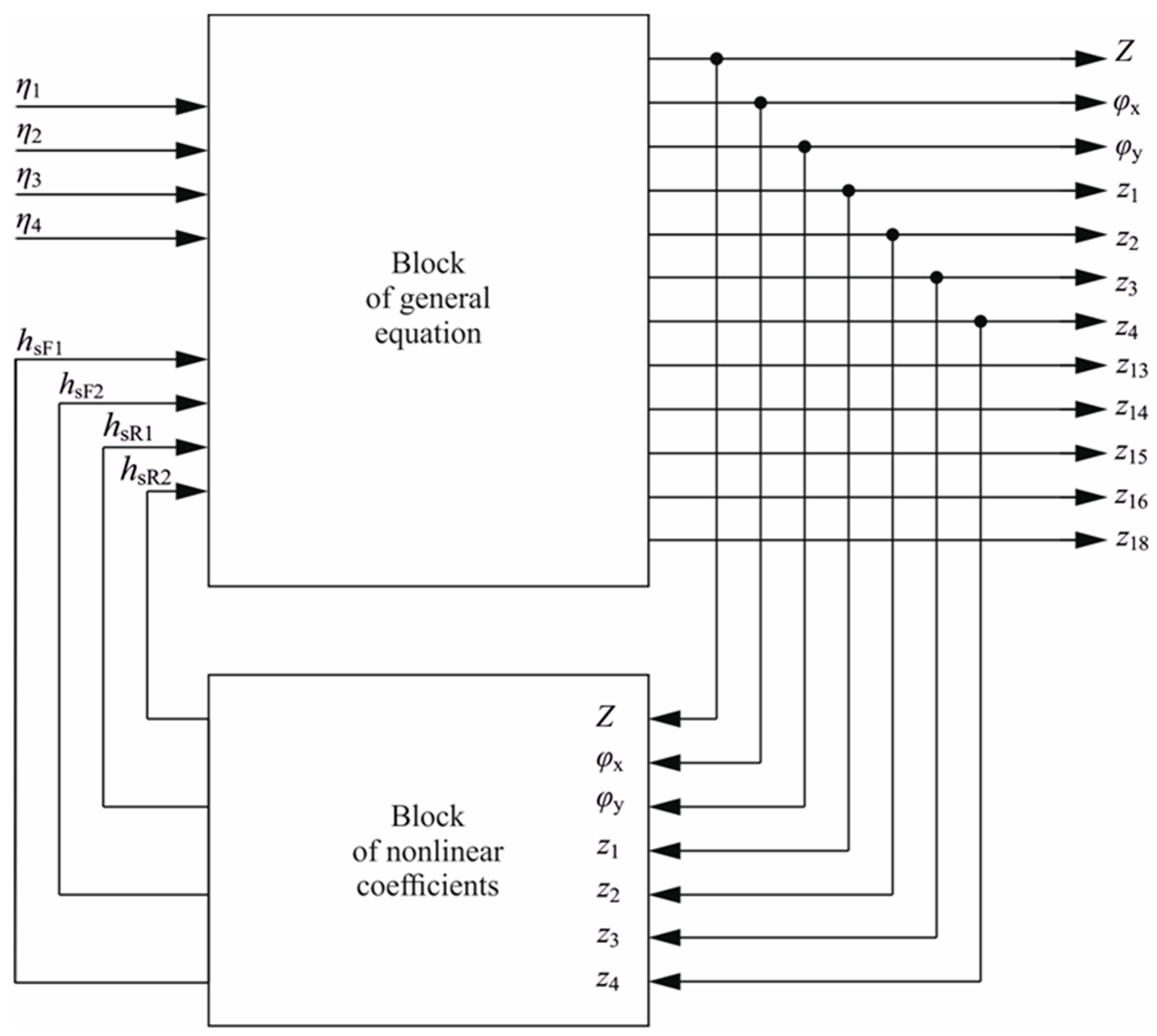
3.2. Damping Law Optimization

The damping coefficient value is constant in common suspension vibration control systems. However, when kinematic excitation characteristics are changing, and the mass of the car (due to passengers or baggage) is changing, permanent damping becomes sub-optimal for all cases. To ensure the comfort of passengers for any case of mass presented in a car, the dependencies of damped and non-damped masses velocities on vibration velocity, should be known. From the theory of vibrations, it is known that the value of the damping coefficient, when the vibration energy is non-permanent, is a function of the vibration speed. The simplest and most logical function is polynomial, in which the damping coefficient depends on the vibration velocity and acceleration. As expected, such damping coefficients show much better results from the model, than permanent damping coefficients. Therefore, the damping coefficient was evaluated by second order polynomial. A higher-order polynomial was not applied, because the coefficient, P₃, appeared to be close to zero in the early modelling results. Therefore, the damping law was optimized, using a second order polynomial:

$$h_{sF1}=P_0+P_1\cdot a_{rel}+P_2\cdot a_{rel}^2$$

(8)

where $a_{rel}={\ddot{z}}_5-{\ddot{z}}_1$. Damping coefficients, h_sF2, h_sR1, h_sR2, were equal to h_sF1.

Parameter P₀ was changed a little, using data from the manufacturer (constant damping coefficient was h_SF1 = 7500 Ns/m). Using this value, the resulting damping force (F_LF) and the acceleration of the driver’s body in the car (Z₁₃) were calculated, and the optimal value of P₀ (when F_LF is highest, and Z₁₃ is lowest) was observed. The coefficient, P₁, was found in the same way; however, in this case, the P₀ value was constant. The coefficient, P₂, was calculated with constant P₀ and P₁ values, which were determined as optimal.

4. Results and Discussion

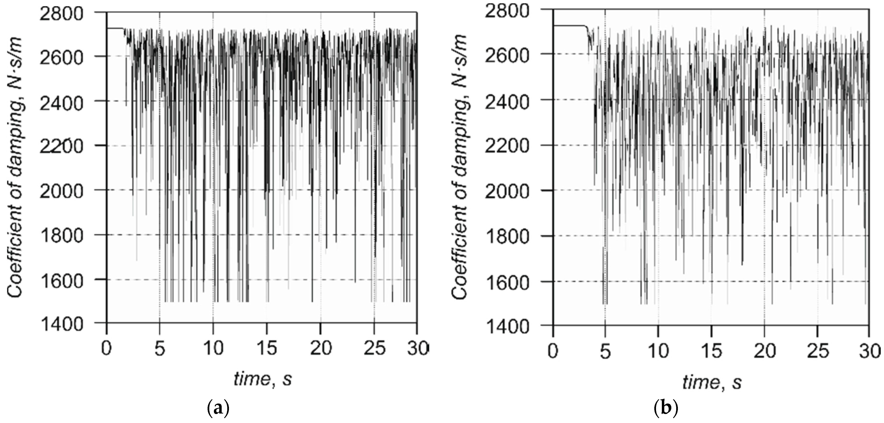
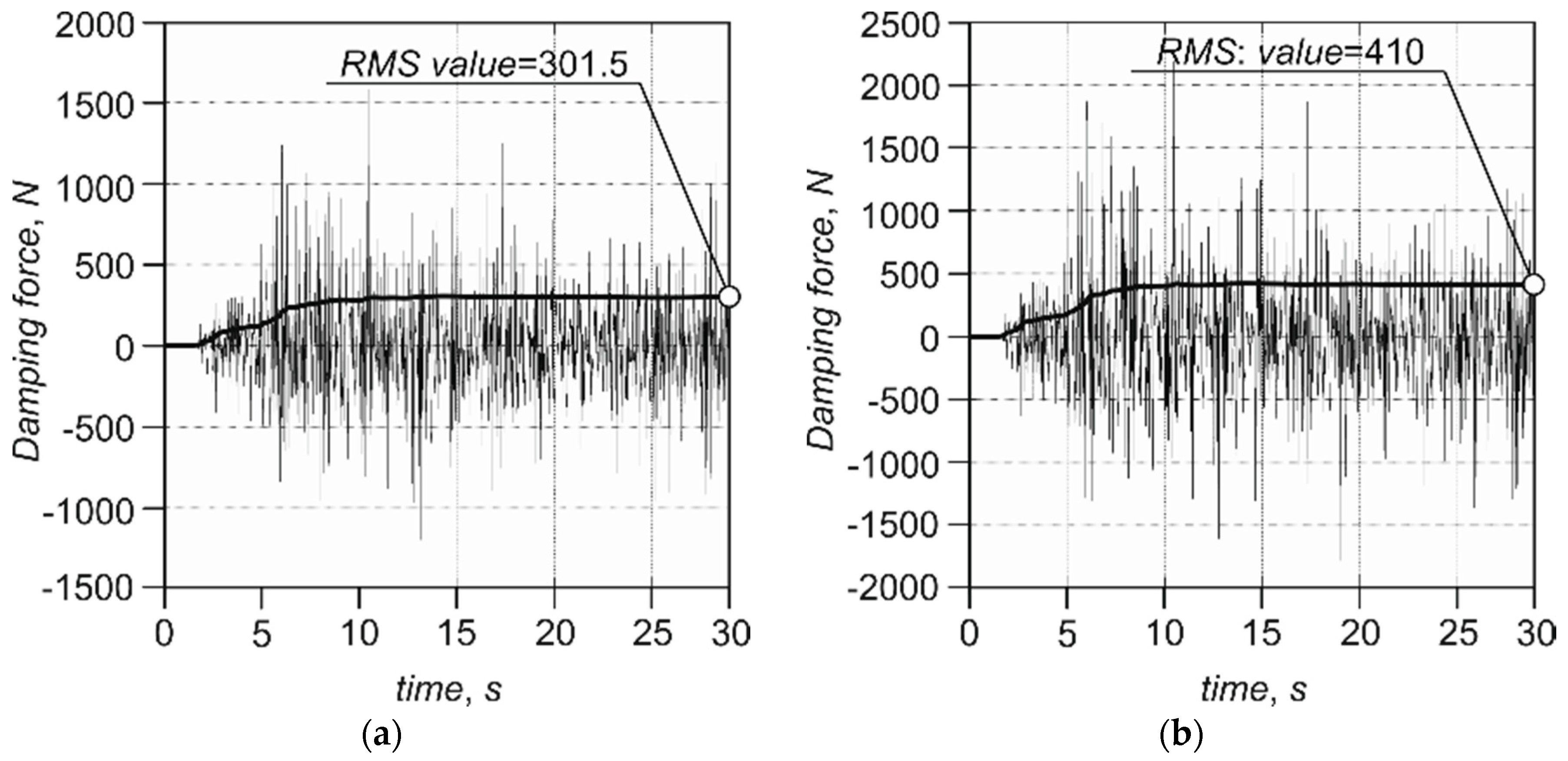
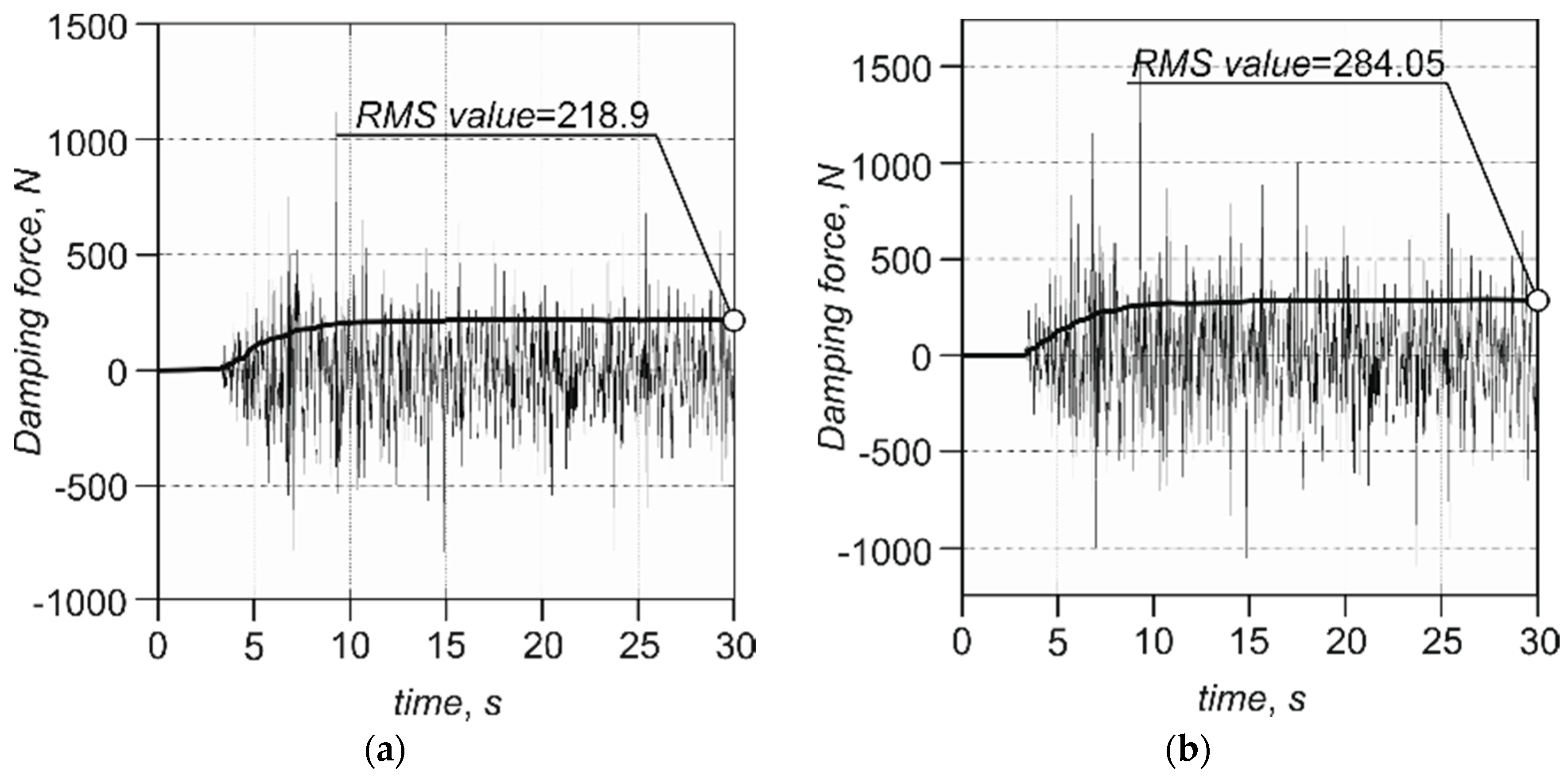
4.1. Experimental Results

To generate the data for the model input, the experiments on roads of different roughness were performed (Figure 4). Road no. 6 showed displacement changes in the range of ±50 mm and road no. 3 showed displacement changes in the range of ±25 mm.

The experimental results (Figure 4) were compared with those of the theoretical model in Figure 5. The damping force from the measured suspension position, while driving at a speed of 60 kph on road no. 3, was calculated by Equation (1). The value of the damping coefficient in the model was the same as used in the car (h_SF1 = 7500 Ns/m). It was found that root mean square (RMS) calculated from experimental data and the model, were in the same range—2000–2000 N.

4.2. Theoretical Results

Numerical simulations were performed using the parameter values, revealed in Table 1. In the simulation, passengers and baggage were eliminated, to get correct results that coincided with experimental research. Experiments were performed without passengers and baggage box masses, thus, the results from the model and experiments were comparable. It is possible to evaluate passengers and baggage box masses, if needed.

Experimentally observed road profiles were used as model inputs (Figure 5). Results of the analysis were evaluated by two parameters: signal extremities and RMS over time. The peaks are important for evaluating the maximum possible impacts to the vehicle suspension system. The level of vibration or dominating force were evaluated by RMS values. The damping power for each road was calculated with both constant damping coefficients (h_SF1 = 7500 Ns/m) and optimized by Equation (7). The calculated damping power for road no. 6 is shown in Figure 6. The optimized damping law gave the possibility of harvesting more power from vibration—the power RMS with optimized damping law was 407.5 W, while permanent damping gave 301.3 W of power. When the roughness was lower (road no. 3), the optimized damping law had a lesser influence on damping power (Figure 7): permanent damping gave 218.7 W, while optimized damping law gave 284.4 W. The higher damping power meant that more energy could be harvested from the shock absorber, therefore, from comparing the results of common and optimized damping controls, we can conclude that our method is effective even on roads with low levels of roughness. In the literature, smaller damping power values have been provided: 19 W [42], 33 W [43] and 40.4 W [44]. Cassidy et al proposed an electromechanical transducer, which generated over 100 W of power [45]. Our device simulated power was higher by several fold (from 15 (at 19 W) to 2.84-fold (at 100 W)). However, comparing the damping power observed using different devices is not appropriate; authors designed their own damper-harvester systems with different control conceptions and different designs. Experiments were performed on different road roughness and at different speeds. Therefore, we can only compare results which show improvement using the same device control as in the current study—we observed 26% more power on roads with high roughness, and 23% more power on medium roughness roads, when the optimized control law was applied.

The coefficients of damping dependencies, over time, for roads of different roughness, with optimized damping laws, are shown in Figure 8. The damping system adapts to the road roughness and creates more comfort for passengers. At the same time, the energy dissipated in the damper, could be more accurately harvested than in classical energy harvesters. Compared to research by Tang et al., where the damping coefficient was observed as 1680–2142 Ns/m [43], which is in good agreement with our research.

The damping force was calculated for each road with different roughness and different damping laws. It was found that for road no. 6, with permanent damping, the force RMS value was 301.5 N, while the optimized law RMS value was 410 N (Figure 9). For road no. 3, permanent damping gave a force of 218.9 N, while optimized damping gave 284.05 N (Figure 10). The results were similar to the harvested power: the optimized damping law had more influence on road no. 6, which was coarser than road no. 3. Chen et al. observed damping forces in the range of −600 to 600 N [46], while Cassidy et al. observed quite a high maximal force of 1 kN [45]. Our forces were calculated in RMS; therefore, they were a little bit lower compared to those measured by other authors. However, our maximal forces were in agreement with other research.

5. Conclusions

Limitations in the common damping control system with constant damping coefficients, motivated us to propose a new method to control automobile suspension vibrations. The polynomial damping law allowed us to find the optimal damping coefficient, whose application to a suspension system resulted in diminished accelerations of the car body and an increased level of comfort for passengers. Also, the application of polynomial damping can increase a lifetime of the car and decrease the development of various defects in the car body and equipment. RMS values for accelerations on road no. 3 decreased by up to 20%, in comparison with classical shock absorbers. Controlled damping increased dissipated power of damped vibrations in a similar range. At a speed of 60 kph, the Range Rover Evoque could reach 400 W RMS for one shock absorber. This case was characterized by a very rough road; nevertheless, 200 W in vibrations is achievable for the majority of test cases. An increase in damping efficiency will significantly increase the load on suspension elements and consequently the damping power. Damping power can be a good diagnostic feature for damping efficiency. Different behaviors of shock absorbers, placed in the same car, can specify problems in the suspension. The damping coefficient change is assumed to be self-adjusted, so a rapid change in road conditions, such as an accidental bump, will be better treated. Our device simulated power was higher by several fold (from 15 (at 19 W) to 2.84 times (at 100 W)). Maximal forces were in agreement with another author’s research.

The estimated need for power is 12 W, which includes control of the shock absorber itself and the powering of data processing, and data transmitting units, which are usually used in automobiles. Therefore, our control method can be applied to harvest more energy than in common shock absorbers, and to power electronic devices.

References

1. Cassidy, I.L.; Scruggs, J.T.; Behrens, S.; Gavin, H.P. Design and experimental characterization of an electromagnetic transducer for large-scale vibratory energy harvesting applications. J. Intell. Mater. Syst. Struct. 2011, 22, 2009–2024. [Google Scholar] [CrossRef]
2. Zhu, S.; Shen, W.-A.; Xu, Y.-L. Linear electromagnetic devices for vibration damping and energy harvesting: Modeling and testing. Eng. Struct. 2012, 34, 198–212. [Google Scholar] [CrossRef]
3. Tang, X.; Zuo, L. Simultaneous energy harvesting and vibration control of structures with tuned mass dampers. J. Intell. Mater. Syst. Struct. 2012, 23, 2117–2127. [Google Scholar] [CrossRef]
4. Ali, S.F.; Adhikari, S. Energy harvesting dynamic vibration absorbers. J. Appl. Mech. 2013, 80, 41004. [Google Scholar] [CrossRef]
5. Gonzalez-Buelga, A.; Clare, L.; Cammarano, A.; Neild, S.; Burrow, S.; Inman, D. An optimised tuned mass damper/harvester device. Struct. Control Health Monit. 2014, 21, 1154–1169. [Google Scholar] [CrossRef] [Green Version]
6. Zhu, J.; Zhang, W. Coupled analysis of multi-impact energy harvesting from low-frequency wind induced vibrations. Smart Mater. Struct. 2015, 24, 45007. [Google Scholar] [CrossRef]
7. Madhav, C.; Ali, S.F. Harvesting Energy from Vibration Absorber under Random Excitations. IFAC-Pap. 2016, 49, 807–812. [Google Scholar] [CrossRef]
8. Salvi, J.; Giaralis, A. Concept Study of A Novel Energy Harvesting-Enabled Tuned Mass-Damper-Inerter (EH-TMDI) Device for Vibration Control of Harmonically-Excited Structures. J. Phys. Conf. Ser. 2016, 744, 012082. [Google Scholar] [CrossRef]
9. Luo, Y.; Sun, H.; Wang, X.; Zuo, L.; Chen, N. Wind Induced Vibration Control and Energy Harvesting of Electromagnetic Resonant Shunt Tuned Mass-Damper-Inerter for Building Structures. Shock Vib. 2017, 2017, 1–13. [Google Scholar] [CrossRef]
10. Takeya, K.; Sasaki, E.; Kobayashi, Y. Design and parametric study on energy harvesting from bridge vibration using tuned dual-mass damper systems. J. Sound Vib. 2016, 361, 50–65. [Google Scholar] [CrossRef]
11. Awrejcewicz, J.; Olejnik, P. Active control of two degrees-of-freedom building-ground system. Arch. Control Sci. 2007, 17, 393–408. [Google Scholar]
12. Liao, Y.; Sodano, H.A. Model of a single mode energy harvester and properties for optimal power generation. Smart Mater. Struct. 2008, 17, 65026. [Google Scholar] [CrossRef]
13. Simon, P.; Yves, S.-A. Improving the performance of a piezoelectric energy harvester using a variable thickness beam. Smart Mater. Struct. 2010, 19, 105020. [Google Scholar]
14. Bucinskas, V. Energy Harvesting Shock Absorber and Method for Controlling Same. U.S. Patent 20140027217 A1, 30 January 2014. [Google Scholar]
15. Bucinskas, V.; Klevinskis, A.; Sesok, N.; Iljin, I.; Warsza, Z.L. Evaluation of damping characteristics of a damper with magneto-rheological fluid. In Advanced Mechatronics Solutions; Jablonski, R., Brezina, T., Eds.; Springer: Cham, Switzerland, 2016; pp. 411–420. [Google Scholar]
16. Mitrouchev, P.; Klevinskis, A.; Bucinskas, V.; Dragasius, E.; Udris, D.; Morkvenaite-Vilkonciene, I. Analytical research of damping efficiency and heat generation of magnetorheological damper. Smart Mater. Struct. 2017, 26, 65026. [Google Scholar] [CrossRef]
17. Lei, Z.; Brian, S.; Jurgen, S.; Yu, Z. Design and characterization of an electromagnetic energy harvester for vehicle suspensions. Smart Mater. Struct. 2010, 19, 45003. [Google Scholar]
18. Abed, I.; Kacem, N.; Bouhaddi, N.; Bouazizi, M.L. Multi-modal vibration energy harvesting approach based on nonlinear oscillator arrays under magnetic levitation. Smart Mater. Struct. 2016, 25, 25018. [Google Scholar] [CrossRef]
19. Kacem, N.; Baguet, S.; Hentz, S.; Dufour, R. Nonlinear phenomena in nanomechanical resonators: Mechanical behaviors and physical limitations. Mech. Ind. 2010, 11, 521–529. [Google Scholar] [CrossRef]
20. Czop, P.; Sławik, D. A high-frequency first-principle model of a shock absorber and servo-hydraulic tester. Mech. Syst. Signal Process. 2011, 25, 1937–1955. [Google Scholar] [CrossRef]
21. Lam, A.H.-F.; Liao, W.-H. Semi-active control of automotive suspension systems with magneto-rheological dampers. Int. J. Veh. Des. 2003, 33, 50–75. [Google Scholar] [CrossRef]
22. Lee, H.-S.; Choi, S.-B. Control and response characteristics of a magneto-rheological fluid damper for passenger vehicles. J. Intell. Mater. Syst. Struct. 2000, 11, 80–87. [Google Scholar] [CrossRef]
23. Li, S.; Lu, Y.; Li, L. Dynamical test and modeling for hydraulic shock absorber on heavy vehicle under harmonic and random loadings. Res. J. Appl. Sci. Eng. Technol. 2012, 4, 1903–1910. [Google Scholar]
24. Worden, K.; Hickey, D.; Haroon, M.; Adams, D.E. Nonlinear system identification of automotive dampers: A time and frequency-domain analysis. Mech. Syst. Signal Process. 2009, 23, 104–126. [Google Scholar] [CrossRef]
25. Zubieta, M.; Elejabarrieta, M.J.; Bou-Ali, M.M. Characterization and modeling of the static and dynamic friction in a damper. Mech. Mach. Theory 2009, 44, 1560–1569. [Google Scholar] [CrossRef]
26. Lajqi, S.; Pehan, S. Designs and optimizations of active and semi-active non-linear suspension systems for a terrain vehicle. Stroj. Vestnik J. Mech. Eng. 2012, 58, 732–743. [Google Scholar] [CrossRef]
27. Mangal, S.K.; Kumar, A. Geometric parameter optimization of magneto-rheological damper using design of experiment technique. Int. J. Mech. Mater. Eng. 2015, 10, 4. [Google Scholar] [CrossRef]
28. Hudha, K.; Jamaluddin, H.; Samin, P.M.; Rahman, R.A. Non-parametric linearised data driven modelling and force tracking control of a magnetorheological damper. Int. J. Veh. Des. 2008, 46, 250–269. [Google Scholar] [CrossRef]
29. Muhammad, A.; Yao, X.-L.; Deng, Z.-C. Review of magnetorheological (MR) fluids and its applications in vibration control. J. Mar. Sci. Appl. 2006, 5, 17–29. [Google Scholar] [CrossRef]
30. Sapiński, B.; Rosół, M.; Węgrzynowski, M. Investigation of an energy harvesting MR damper in a vibration control system. Smart Mater. Struct. 2016, 25, 125017. [Google Scholar] [CrossRef]
31. Jastrzębski, Ł.; Sapiński, B. Electrical interface for an MR damper-based vibration reduction system with energy harvesting capability. In Proceedings of the IEEE 18th International Carpathian Control Conference (ICCC), Sinaia, Romania, 28–31 May 2017; pp. 189–192. [Google Scholar]
32. Hu, G.; Tang, L.; Banerjee, A.; Das, R. Metastructure With Piezoelectric Element for Simultaneous Vibration Suppression and Energy Harvesting. J. Vib. Acoust. 2017, 139, 11012. [Google Scholar] [CrossRef]
33. Hu, G.; Tang, L.; Das, R. Metamaterial-inspired piezoelectric system with dual functionalities: Energy harvesting and vibration suppression, Active and Passive Smart Structures and Integrated Systems. In Proceedings of the International Society for Optics and Photonics, Portland, OR, USA, 11–16 April 2017; p. 101641X. [Google Scholar]
34. Bowden, J.A.; Burrow, S.G.; Cammarano, A.; Clare, L.R.; Mitcheson, P.D. Switched-mode load impedance synthesis to parametrically tune electromagnetic vibration energy harvesters. IEEE/ASME Trans. Mechatron. 2015, 20, 603–610. [Google Scholar] [CrossRef]
35. Mitcheson, P.D.; Toh, T.T.; Wong, K.H.; Burrow, S.G.; Holmes, A.S. Tuning the resonant frequency and damping of an electromagnetic energy harvester using power electronics. IEEE Trans. Circuits Syst. II 2011, 58, 792–796. [Google Scholar] [CrossRef]
36. Balato, M.; Costanzo, L.; Vitelli, M. Resonant electromagnetic vibration harvesters: Determination of the equivalent electric circuit parameters and simplified closed-form analysis for the identification of the optimal diode bridge rectifier DC load. Int. J. Electr. Power Energy Syst. 2017, 84, 111–123. [Google Scholar] [CrossRef]
37. Balato, M.; Costanzo, L.; Vitelli, M. Maximization of the extracted power in resonant electromagnetic vibration harvesters applications employing bridge rectifiers. Sens. Actuators A 2017, 263, 63–75. [Google Scholar] [CrossRef]
38. Bakar, S.A.A.; Jamaluddin, H.; Rahman, R.A.; Samin, P.M.; Masuda, R.; Hashimoto, H.; Inaba, T. Modelling of magnetorheological semi-active suspension system controlled by semi-active damping force estimator. Int. J. Comput. Appl. Technol. 2011, 42, 49–64. [Google Scholar] [CrossRef]
39. Goncalves, F.D.; Ahmadian, M. A hybrid control policy for semi-active vehicle suspensions. Shock Vib. 2003, 10, 59–69. [Google Scholar] [CrossRef]
40. Ahmadian, M.; Vahdati, N. Transient dynamics of semiactive suspensions with hybrid control. J. Intell. Mater. Syst. Struct. 2006, 17, 145–153. [Google Scholar] [CrossRef]
41. Wang, W.L.; Yang, X.J.; Xu, G.X.; Huang, Y. Multi-objective design optimization of the complete valve system in an adjustable linear hydraulic damper. Proc. Inst. Mech. Eng. Part C J. Mech. Eng. Sci. 2011, 225, 679–699. [Google Scholar] [CrossRef]
42. Li, Z.; Zuo, L.; Luhrs, G.; Lin, L.; Qin, Y.-X. Electromagnetic energy-harvesting shock absorbers: Design, modeling, and road tests. IEEE Trans. Veh. Technol. 2013, 62, 1065–1074. [Google Scholar] [CrossRef]
43. Tang, X.; Lin, T.; Zuo, L. Design and optimization of a tubular linear electromagnetic vibration energy harvester. IEEE/ASME Trans. Mechatron. 2014, 19, 615–622. [Google Scholar] [CrossRef]
44. Li, Z.; Zuo, L.; Kuang, J.; Luhrs, G. Energy-harvesting shock absorber with a mechanical motion rectifier. Smart Mater. Struct. 2012, 22, 25008. [Google Scholar] [CrossRef]
45. Cassidy, I.L.; Scruggs, J.T.; Behrens, S. Design of electromagnetic energy harvesters for large-scale structural vibration applications. In Proceedings of the Society of Photo-Optical Instrumentation Engineers 7977, Active and Passive Smart Structures and Integrated Systems, San Diego, CA, USA, 27 April 2011; p. 79770P. [Google Scholar]
46. Chen, C.; Liao, W.-H. A self-sensing magnetorheological damper with power generation. Smart Mater. Struct. 2012, 21, 25014. [Google Scholar] [CrossRef]
Figure 1. Experimental equipment; 1 and 2 represent accelerometers.
Energies 10 01742 g001
Figure 2. Dynamic model of the car body. CG—center of gravity; Z—coordinate of the vertical axis; X and Y—coordinates of horizontal axes; φx and φy are the rotation angles about the axes X and Y, respectively; xs, ys and zs—coordinates of CG with respect to the center of stiffness; z1, z2, z3, z4—the coordinates of vertical movements of wheels; z5, z6, z7, z8—auxiliary coordinates at the shock absorbers’ points, z9, z10, z11, z12—the points of seat contact with the passengers’ bodies and z17—the point of the luggage compartment; z13z16—coordinates of the center of masses of the driver and three passengers, respectively, z18—coordinate of center of mass of baggage in the baggage box; M—mass of the car; Jx and Jy—the moments of inertia about the respective axis; Jxy—the mixed moment; ksF—stiffness coefficients of the front wheel suspension of individual elastic elements; ksR—stiffness coefficients of the rear wheel suspension of individual elastic elements; hsF1, hsF2, hsR1, hsR2—the damping coefficients; mwF and mwR—the suspension mass and the rear mass; ksF and ksR—the front and the rear wheel tires spring elements coefficients of stiffness, respectively; hsF and hsR—the coefficients of damping for the front and the rear wheel, respectively; m1, m2, m3, m4, mwmasses, kuz1, kuz2, kuz3, kuz4, kg—coefficients of stiffness, and huz1, huz2, huz3, huz4, hg—damping coefficients of the driver, three passengers and load in the baggage box, respectively; L1, ..., L14—distances; η1, η2, η3, η4—coordinates, at which the dynamic system (the car) was excited kinematically.
Energies 10 01742 g002
Figure 3. General structure of the dynamic model of the car.
Energies 10 01742 g003
Figure 4. Road displacement dependencies on time, observed experimentally: (a) road no. 6; (b) road no. 3.
Energies 10 01742 g004
Figure 5. Experimental and analytical damping forces, F represents force.
Energies 10 01742 g005
Figure 6. Damping power dependencies over time, obtained from the model for road no. 6: (a) Permanent damping with hSF1 = 7500 Ns/m; (b) Optimized damping law. RMS—root mean square.
Energies 10 01742 g006
Figure 7. Damping power dependencies on time, obtained from the model for road no. 3: (a) Permanent damping with hSF1 = 7500 Ns/m; (b) Optimized damping law.
Energies 10 01742 g007
Figure 8. Coefficients of damping (hSF1) with optimized damping law dependencies, over time: (a) for road no. 6, P0 = 5765, P1 = −19, P2 = 0.5; (b) for road no. 3; P0 = 5050, P1 = 30, P2 = 0.45.
Energies 10 01742 g008
Figure 9. Damping force dependencies, over time, for road no. 6: (a) with permanent damping (hSF1 = 7500 Ns/m); (b) with the optimized damping law.
Energies 10 01742 g009
Figure 10. Damping force dependencies, over time, for road no. 3: (a) with permanent damping (hSF1 = 7500 Ns/m); (b) with the optimized damping law.
Energies 10 01742 g010