Modular Multilevel Converters: Control and Applications

Abstract

This review article is mainly oriented to the control and applications of modular multilevel converters (MMC). The main topologies of the switching modules are presented, for normal operation and for the elimination of DC faults. Methods to keep the capacitor voltage balanced are included. The voltage and current modulators, that are the most internal loops of control, are detailed. Voltage control and current control schemes are included which regulate DC link voltage and reactive power. The cases of unbalanced and distorted networks are analyzed, and schemes are proposed so that MMC contribute to improve the quality of the grid in these situations. The main applications in high voltage direct current (HVDC) transmission along with other medium voltage (MV) and low voltage (LV) applications are included. Finally, the application to offshore wind farms is specifically analyzed.

1. Introduction

High voltage direct current (HVDC) transmission was historically performed using the thyristor-controlled Line Commutated Converter (LCC) [1]. However, it has several limitations: it uses semiconductors that cannot be switched off autonomously, external voltage must supply reactive power to produce semiconductor switching, it only operates with a delay power factor and it cannot be used in isolated systems [2].

Later, the Voltage Source Converter (VSC) [3], made with insulated gate bipolar transistors (IGBT), was used. This has several advantages over LCC: it uses semiconductors that can be switched on and off autonomously, the converter can supply reactive power, it can operate with a delay and advance power factor and it can be used in isolated systems [2].

When the two level VSC topology is used, it presents several problems:

(1)

Very high di/dt of the arms of the converter and the semiconductors.

(2)

Great stress and over-voltages in the semiconductors.

(3)

Emission of electromagnetic radiation and difficulties in the construction of the converter.

(4)

With pulse-width modulation (PWM): great loss of power in the semiconductors and use of voluminous and expensive passive filters.

(5)

As capacity is concentrated, DC short-circuits are very difficult to limit.

To improve these aspects, multi-level VSC has been used [4]. However, it has severe limitations such as insufficient industrial scalability and limited number of voltage levels [5]. The modular multilevel converter (MCC) (Figure 1), presented for the first time by Lesnicar and R. Marquardt [6], improves these problems notably [7]:

(1)

The arm current flows continuously, avoiding the high di/dt of the VSC switching.

(2)

There is a great reduction of power losses and filtering needs.

(3)

The capacity is distributed among the modules of each arm.

(4)

The complexity does not increase substantially with the number of levels employed.

(5)

The fault currents in the DC side are smaller, making them more suitable for multi-terminal HVDC grids.

Although publications on MMC have been made in very different orientations, this article is oriented towards control and applications, so some important aspects such as reduction of circulating currents [8,9,10,11] or modeling of the converter is not included [12,13,14,15].

Since the MMC is a multi-level converter, the voltage harmonics generated are smaller than in a two-level converter, thus reducing the values of the reactive components of the filter, which can even be eliminated in some cases. When a large number of modules is used, the switching frequency of the modules is reduced and the converter switching losses are minimized [16].

When the distance is long (greater than 400–700 km on land, and 50–60 km at sea) DC transmission is cheaper than AC transmission. DC transmission needs fewer cables, but requires the presence of electronic converters. Another limitation of AC transmission is the reactive energy that consumes the inductance of the line, which for long distance transmission becomes a fundamental factor. MMC was first commercially used in the Trans Bay Cable project in San Francisco [16].

The article has been organized as follows. Section 2 is devoted to the topologies of the switching modules. Section 3 is dedicated to the fundamental equations relating the voltages and currents of the DC side, AC side, switching modules, arm inductances, and circulating currents. Section 4 is devoted to the balancing of the capacitors of the switching modules. Section 5 includes voltage and current modulators. Section 6 deals with the connection of the converter to balanced, unbalanced or distorted grids. Section 7 includes high voltage (HV), medium voltage (MV), and low voltage (LV) applications. Finally, Section 8 is devoted to the use of MMC in offshore wind farms.

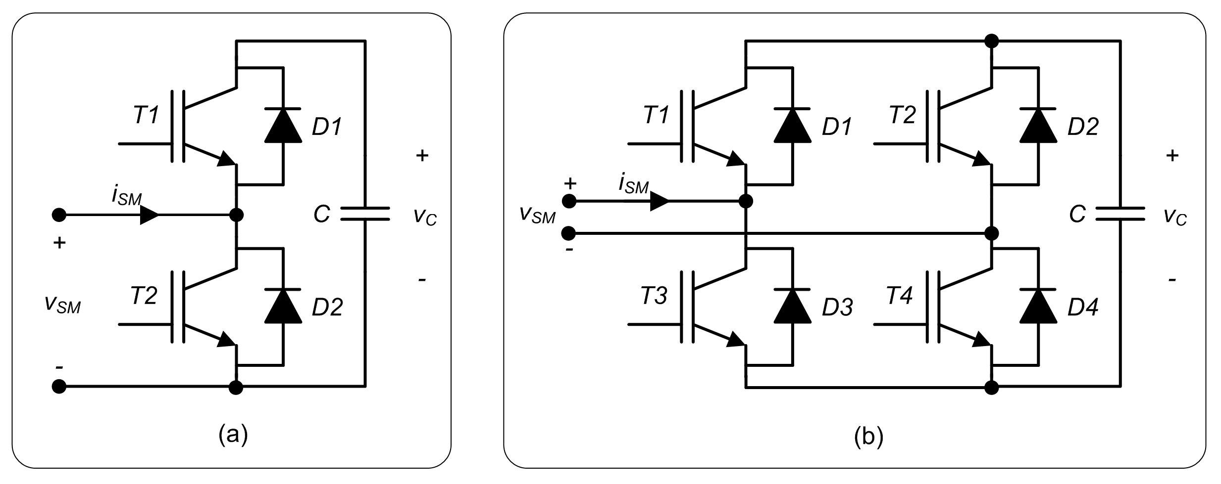
2. Switching Module Topologies

The first topology of a switching module (SM) presented for MMC (by Lesnicar and Marquardt [6]) was the half bridge (HB) topology (Figure 2a), which has been the most used. It consists of two IGBTs, two diodes, and one capacitor. The SM is ON when T1 is ON and T2 is OFF (

Table 1. State of conduction, voltages and currents of the switching module (SM).

SM State	$T_1$ State	$T_2$ State	${\mathit{i}}_{\mathit{S}\mathit{M}}$	$\Delta {\mathit{v}}_{\mathit{C}}$	${\mathit{i}}_{\mathit{S}\mathit{M}}$ Flows Through	${\mathit{v}}_{\mathit{S}\mathit{M}}$
ON	ON	OFF	$>0$	$+$	${\mathrm{D}}_1$	$v_C$
ON	ON	OFF	$<0$	$-$	${\mathrm{T}}_1$	$v_C$
OFF	OFF	ON	$>0$	$0$	${\mathrm{T}}_2$	$0$
OFF	OFF	ON	$<0$	$0$	${\mathrm{D}}_2$	$0$

), while SM is OFF when T1 is OFF and T2 is ON. When the SM is ON, the SM voltage is the same as the SM capacitor voltage, while when it is OFF the voltage is zero. According to the SM state and the direction of the SM current, the current circulates through the capacitor producing its charge/discharge, or it does not circulate through the capacitor, maintaining its voltage.

In the case of a DC short circuit, the HB topology turns OFF all IGBTs, and a fault current occurs, which is the quotient between the AC voltage and the impedance of the arm inductances. The full bridge (FB) topology (Figure 2b) allows an active role in case of failure [5]. This topology behaves just like the HB topology during normal operation. To set the SM to ON ($v_{SM}=v_C$), IGBT 1 and 4 are turned ON. To set the SM to OFF ($v_{SM}=0$), there are two options, set T1 and T3 to ON, or set T2 and T4 to ON. During the fault, a voltage of opposite sign can be introduced in series with that fault to reduce and eliminate it. For example, if the fault current is positive with respect to the SM, T1 and T4 are set to ON so the SM voltage is positive, whereas if the current is negative, T2 and T3 are set to ON so the SM voltage is negative. The problem with the FB topology is that, in order to be able to eliminate faults, the price to be paid is to double the loss of power during normal operation.

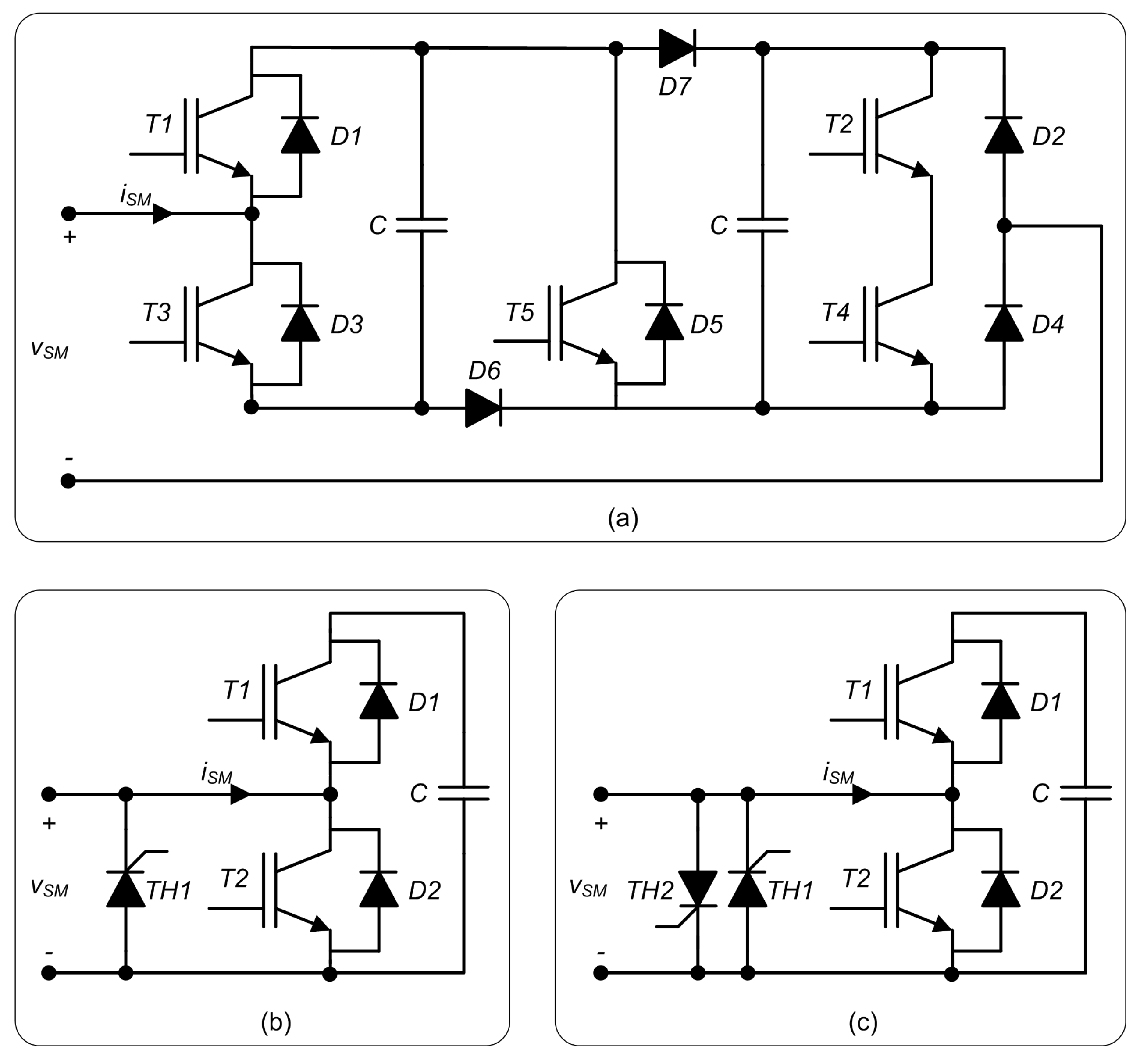
Other topologies that include additional components have been introduced to handle short circuits in the DC part. The Double Clamp Submodule Topology [5] (Figure 3a) is equivalent to two half bridges, plus an additional IGBT T5. In normal operation, IGBT T5 is in conduction, but it is switched off during the DC fault, allowing the two capacitors to oppose the fault.

Other topologies to reduce the impact of short duration of time DC short circuits have included thyristors [17]. The first one includes a thyristor in parallel with D2 (Figure 3b), which is triggered when the fault is detected. Then the current flows through the thyristor instead of D2, due to the higher I²t of the thyristor. The problem is that there is a rectifier effect between the AC and the DC through the diodes D2 of the SMs that feed the DC fault. To avoid this, the topology with two thyristors was proposed (Figure 3c) that causes a short circuit in AC limited by branch inductances; when the DC fault is cleared, the IGBTs take control again.

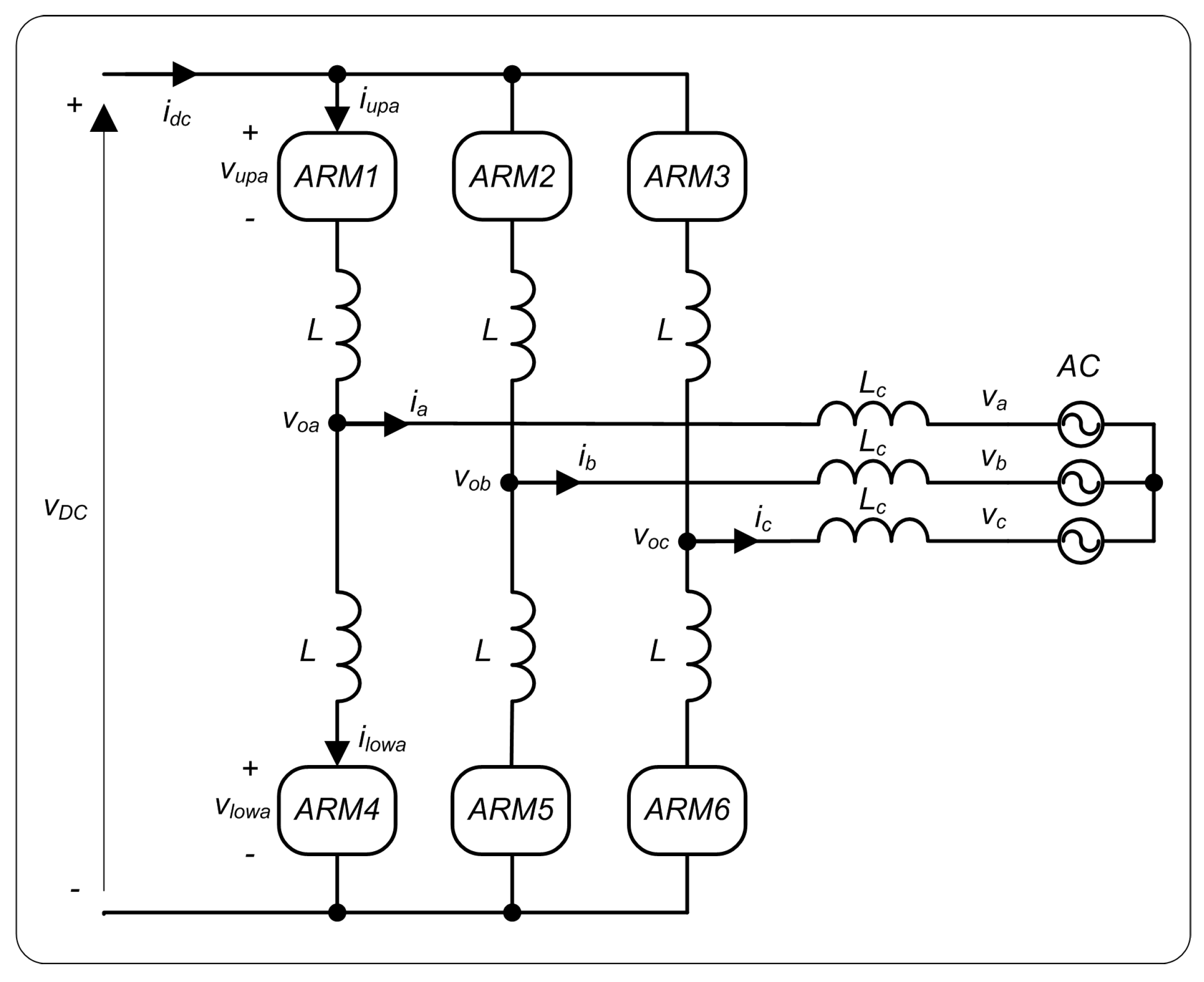
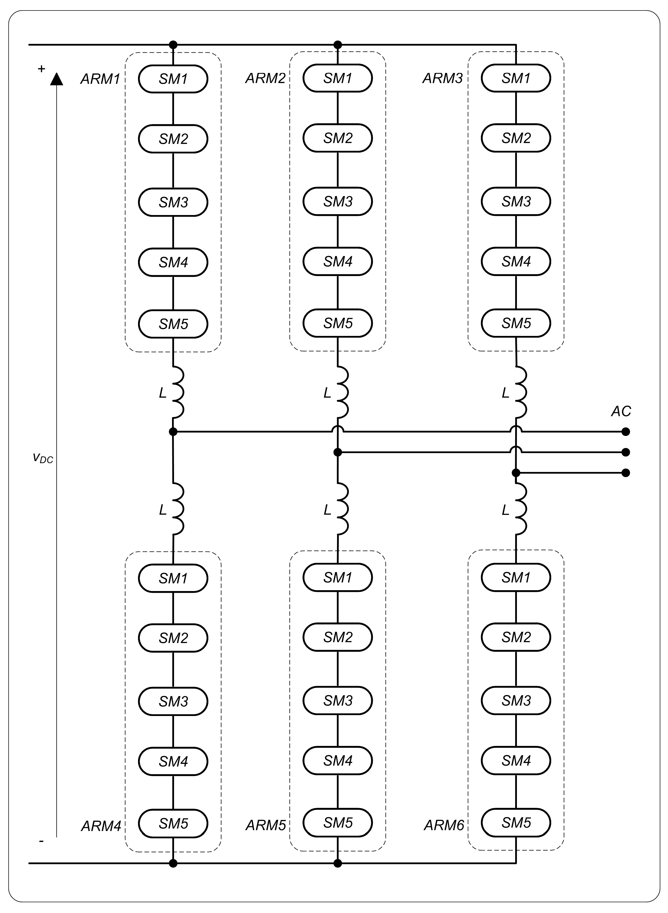
3. Fundamental Equations

The SMs of each phase have been grouped into two blocks with voltages $v_{upa}$ (upper arm) and $v_{lowa}$ (lower arm) (Figure 4). The capacitor of each SM is kept charged with a voltage equal to the DC voltage $V_{DC}$ divided by the number of SMs of each arm $n$, $v_C=\frac{V_{DC}}{n}$. In order for the sum of the voltages of the two arms of a phase to be equal to the DC voltage, the sum of the number of SMs in the ON state in the upper arm $n_{up}$ and lower arm $n_{low}$ of each phase must be equal to $n$:

$$n_{up}+n_{low}=n$$

(1)

The equation relating the DC and AC voltage can be obtained through the upper arm, or the lower arm:

$$v_{oa}=\frac{V_{DC}}{2}-v_{upa}-L\frac{d{i}_{upa}}{dt}$$

(2)

$$v_{oa}=-\frac{V_{DC}}{2}+v_{lowa}+L\frac{d{i}_{lowa}}{dt}$$

(3)

The voltage of each arm, $v_{upa}$ and $v_{lowa}$, depends on the conduction state $1/0$ of each SM, $S_{upak}$, and $S_{lowak}$, and the voltage of each capacitor, $v_{Cupak}$, and $v_{Clowak}$, the sum of the voltages of the modules being:

$$v_{upa}={\displaystyle \sum }_{k=1}^n{S}_{upak}{v}_{Cupak}$$

(4)

$$v_{lowa}={\displaystyle \sum }_{k=1}^n{S}_{lowak}{v}_{Clowak}$$

(5)

For each of the arms, a current (upper $i_{upa}$ and lower $i_{lowa}$) is circulated equal to half the phase current $i_a$, plus a third of the DC current $i_{dc}$, plus the circulating current $i_{za}$ [13,18]:

$$i_{upa}=\frac{i_a}{2}+\frac{i_{dc}}{3}+i_{za}$$

(6)

$$i_{lowa}=-\frac{i_a}{2}+\frac{i_{dc}}{3}+i_{za}$$

(7)

From (6) and (7) the circulating current can be obtained as:

$$i_{za}=\frac{i_{upa}+i_{lowa}}{2}-\frac{i_{dc}}{3}$$

(8)

The sum of the three circulating currents of the three arms/phases is zero:

$$i_{za}+i_{zb}+i_{zc}=0$$

(9)

The output voltage of each AC phase can take $n+1$ different values; for example, if the number of SMs per arm is $n=5$, the number of levels of the AC voltage is 6 and their values can be seen in

Table 2. AC voltages depending on the number of modules in ON state in each arm.

${\mathit{n}}_{\mathit{u}\mathit{p}}$	${\mathit{n}}_{\mathit{l}\mathit{o}\mathit{w}}$	${\mathit{v}}_{\mathit{o}\mathit{a}}$
5	0	$-\frac{V_{DC}}{2}+0\frac{V_{DC}}{5}$
4	1	$-\frac{V_{DC}}{2}+1\frac{V_{DC}}{5}$
3	2	$-\frac{V_{DC}}{2}+2\frac{V_{DC}}{5}$
2	3	$-\frac{V_{DC}}{2}+3\frac{V_{DC}}{5}$
1	4	$-\frac{V_{DC}}{2}+4\frac{V_{DC}}{5}$
0	5	$-\frac{V_{DC}}{2}+5\frac{V_{DC}}{5}$

as a function of the number of modules that are ON in each arm.

4. Capacitor Balancing

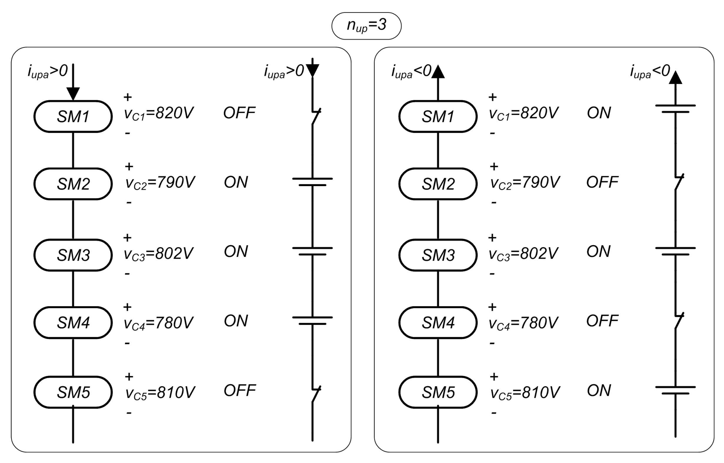
The capacitors of the SMs change their voltage depending on the current flowing through the SM. The voltage of the SM should be kept approximately equal to its theoretical value $\frac{V_{DC}}{n}$. For this, the SM voltage must be measured and the appropriate measures to maintain the voltages in that value must be taken. Otherwise, the capacitor voltages will become more and more unbalanced and the AC output voltage cannot be controlled.

Different types of algorithms have been used to balance capacitor voltages. When a combination of the averaged control and the balanced control is used, it is possible to balance the voltage of the capacitors without using any external circuit [19]. A predictive control, based on minimizing a cost function, allows the capacitor voltages to be balanced, circulating currents to be minimized and the AC currents to be controlled, jointly, under various operating conditions [20]. A method that does not need to measure the current in each arm eliminates current sensors, reducing costs and simplifying the voltage balance control algorithm [21]. The most commonly used algorithm measures the voltages of the capacitors and chooses the SMs that must be ON depending on the direction of the current [7,18]. An example can be seen in Figure 5, in the case of arms with $n=5$ SMs, where the aim is for the capacitor voltages to remain at $800 \mathrm{V}$. Assuming that the desired output voltage is $-\frac{V_{DC}}{2}+2\frac{V_{DC}}{5}=-\frac{4000}{2}+2\frac{4000}{5}=-400 \mathrm{V}$, $n_{up}=3$ and $n_{low}=2$ are required. In the example, the voltages of the upper arm will be balanced, while the lower arm will be balanced in the same way. In the upper arm, three SMs must be set to ON, chosen according to the SM current $i_{upa}$ direction. Depending on whether it is positive/negative, it increases/reduces the voltage of the SMs it circulates. When it is positive, SMs that have less voltage are turned ON to charge, while if negative, the SMs that have the highest voltage are turned ON to discharge.

5. Voltage and Current Modulators

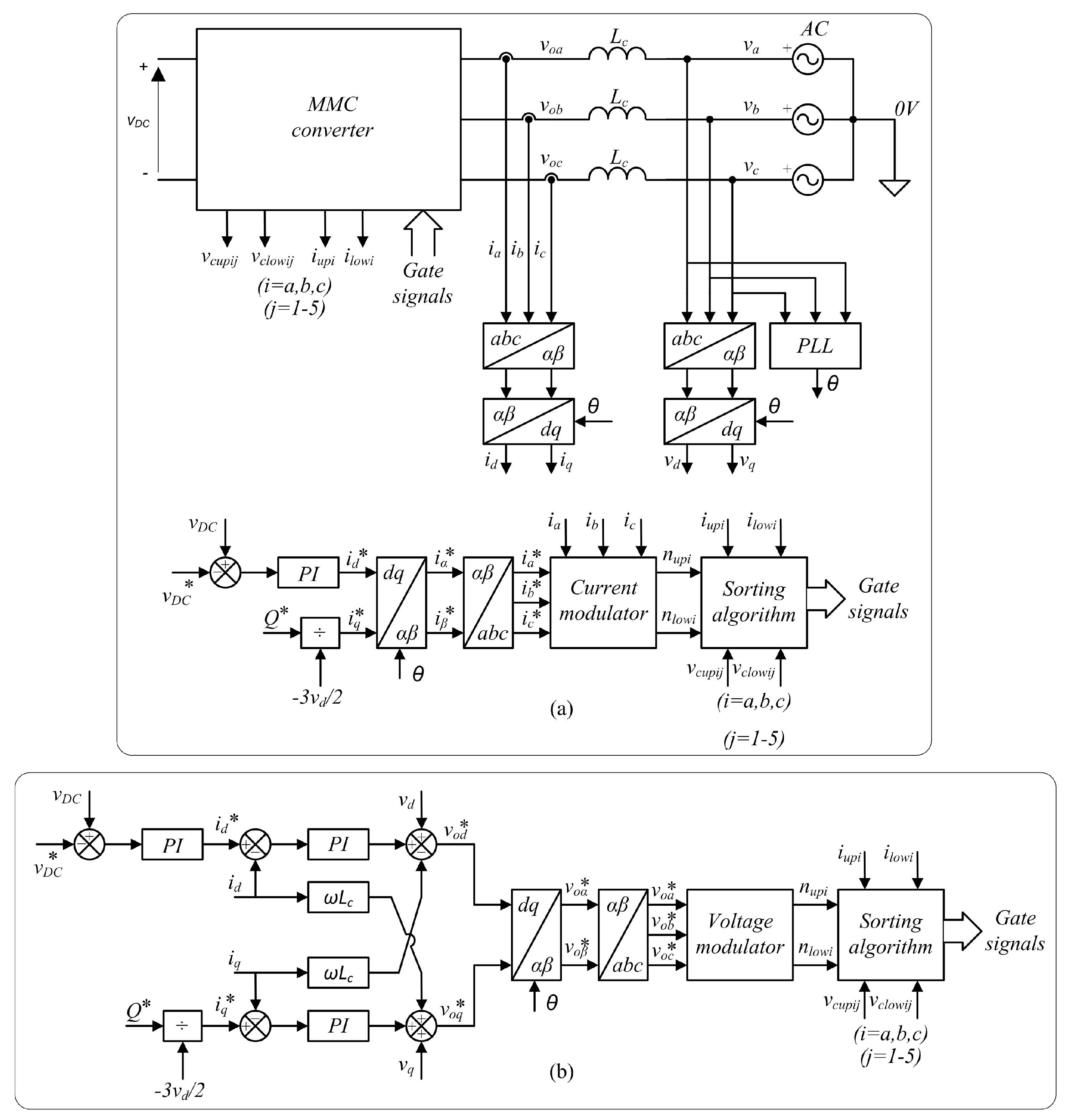
The external control loop of the MMC has two Proportional-Integral (PI) regulators, one for the DC voltage and one for the reactive power exchanged by the AC grid, which generate the grid current references in $dq$ axes. If current control is used, a current modulator is required for the MMC to follow current references. If voltage control is used, two PI regulators are required to transform current references into voltage references and, subsequently, a voltage modulator.

Four voltage modulators and two current modulators are presented in great detail. The former are more commonly used. Their switching frequency is lower. The design of the AC filter is simpler because the switching frequency is constant. The latter have been proposed for applications with greater needs for speed of response.

5.1. Voltage Modulators

The voltage modulators are responsible for calculating the level of the output voltage at each sampling time, depending on the value of the AC voltage reference. When the number of converter levels is small, high-frequency modulation is often used, whereas when the number of levels is high, low-frequency steps are often used. In the first case, the semiconductor switching losses are high. In all cases, the goal is to eliminate or greatly reduce low frequency harmonics to facilitate the filtering of the AC voltage, taking into account the fact that the type of modulation used determines, in part, the harmonics of the generated voltage [22]. First, three voltage modulators using high frequency modulation, phase disposition-sinusoidal PWM, multilevel PWM, and multilevel space vector modulation (SVM) are presented. Finally, the step-level modulator called Near Level Control (NLC) is presented.

The high frequency modulators are presented for the case where each arm consists of $n=5$ SMs, which causes the output voltage between phase and neutral $v_{oabc}$ to have $n+1=6$ levels. The result of the calculation of the modulator will be the number of SMs in the ON state in the upper $n_{up}$ and lower $n_{low}$ arms and, therefore, the output voltage of the corresponding phase will be:

$$v_o=-\frac{V_{DC}}{2}+n_{low}{v}_C$$

(10)

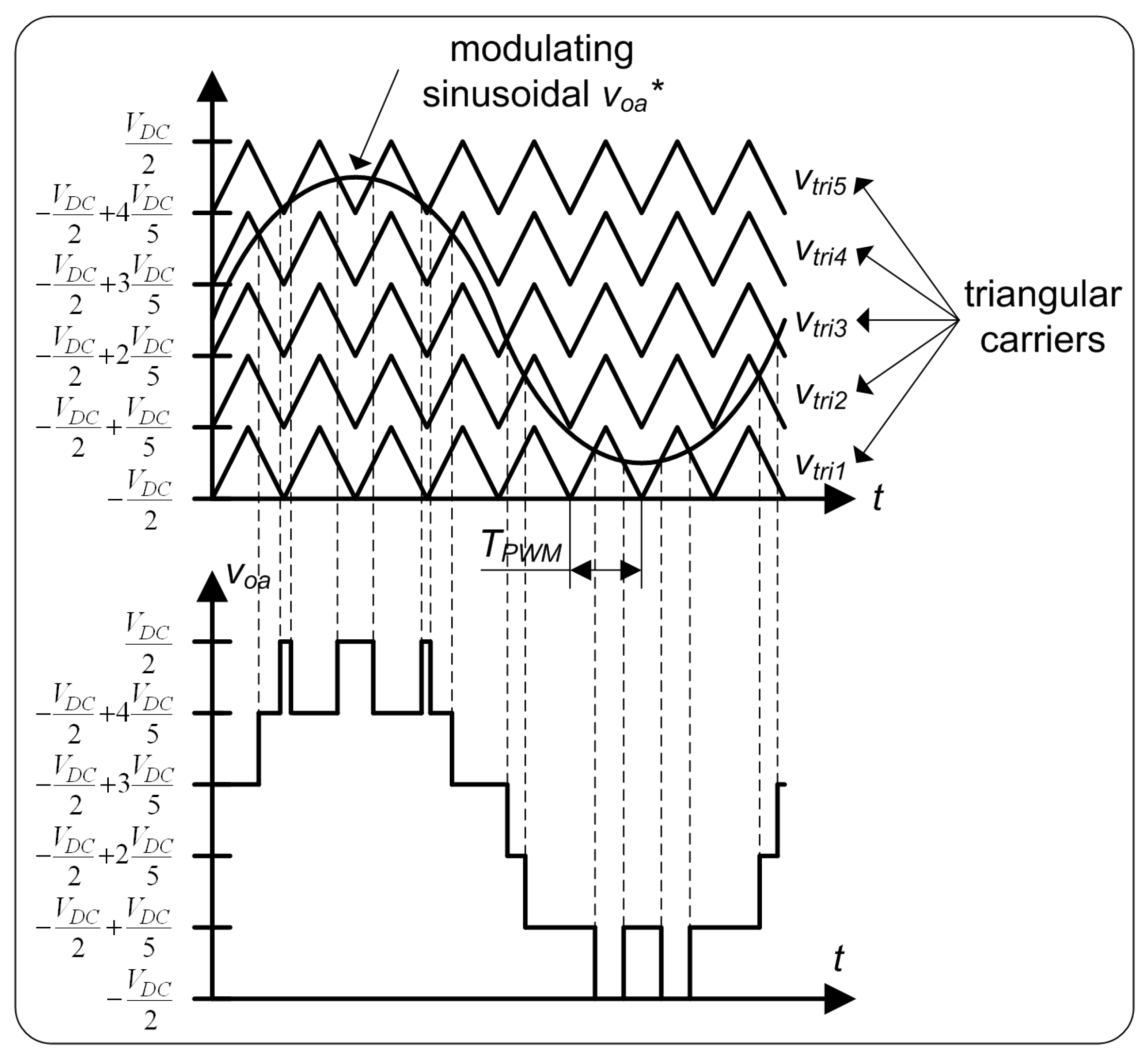
5.1.1. Phase Disposition–Sinusoidal PWM

This is a PWM similar to the one used in a classic two level inverter, but adapted to the case of multilevel converters. In the former, a single high-frequency (carrier) triangle signal is used which is compared to a low-frequency (modulator) sine wave signal. In the second, several high-frequency triangular signals are used (see Figure 6) with a modulating signal to produce the output voltage. It is a modulation that has not been used only in MMC but in multilevel inverters in general. According to the offset between the carriers, there are several types of modulation called [23]: Alternative Phase Opposition Disposition, Phase Disposition, Phase Opposition Disposition, Hybrid, Phase Shifted. The one shown in Figure 6 is Phase Disposition (PD), in which the offset between the carriers is nill.

For the six-level case (Figure 6), the Phase disposition-sinusoidal PWM (PD-SPWM) uses five high frequency carriers. The output voltage takes one of six possible values, $-\frac{V_{DC}}{2},-\frac{V_{DC}}{2}+\frac{V_{DC}}{5},-\frac{V_{DC}}{2}+\frac{2V_{DC}}{5},-\frac{V_{DC}}{2}+\frac{3V_{DC}}{5},-\frac{V_{DC}}{2}+\frac{4V_{DC}}{5},\frac{V_{DC}}{2}$, depending on whether the sinusoidal is higher or lower than each of the triangular ones, as can be seen in the following equation:

$$v_{oa}=\{\begin{array}{c}\frac{V_{DC}}{2}, \left(v_{tri5}<{v_{oa}}^{*}\right)\\ -\frac{V_{DC}}{2}+\frac{4V_{DC}}{5}, \left(v_{tri4}<v_{oa}{}^{*}<v_{tri5}\right)\\ -\frac{V_{DC}}{2}+\frac{3V_{DC}}{5}, \left(v_{tri3}<v_{oa}{}^{*}<v_{tri4}\right)\\ -\frac{V_{DC}}{2}+\frac{2V_{DC}}{5}, \left(v_{tri2}<{v_{oa}}^{*}<v_{tri3}\right)\\ -\frac{V_{DC}}{2}+\frac{V_{DC}}{5}, \left(v_{tri1}<{v_{oa}}^{*}<v_{tri2}\right)\\ -\frac{V_{DC}}{2}, \left({v_{oa}}^{*}<v_{tri1}\right)\end{array}$$

(11)

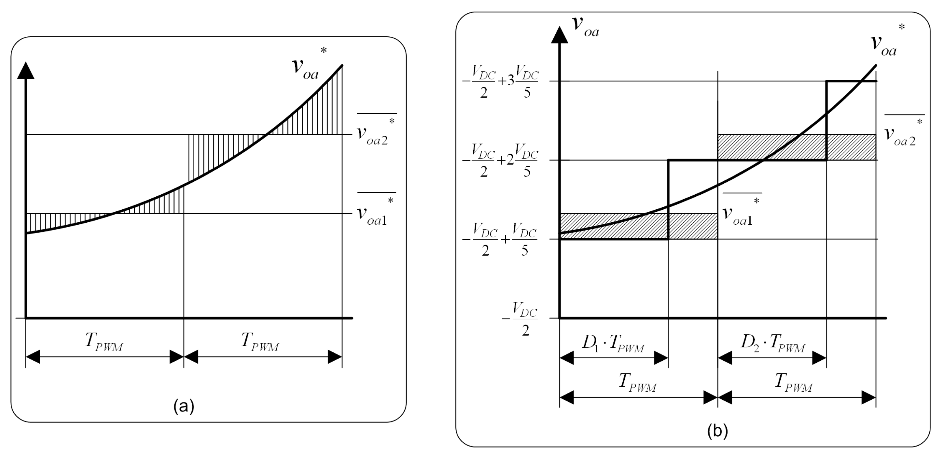
5.1.2. Multilevel PWM

Multilevel PWM is a PWM method that calculates a duty cycle $D_k$ every PWM period $T_{PWM}$ [7]. The PWM period establishes the commutation period of the converter. The duty cycle is calculated so the average values of the output converter voltage $v_{oa}$ and its reference value ${v_{oa}}^{*}$ will be the same in the PWM period $k$, $\overline{v_{oak}}$ and $\overline{{v_{oak}}^{*}}$ respectively. The average value of the reference $\overline{{v_{oak}}^{*}}$ is:

$$\overline{{v_{oak}}^{*}}=\frac{1}{T_{PWM}}\underset{t_k}{\overset{t_{k+1}}{{\displaystyle \int }}}{v_{oa}}^{*}\left(t\right)dt$$

(12)

The output voltage of the converter $v_{oa}$ can take the instantaneous values $-\frac{V_{DC}}{2},-\frac{V_{DC}}{2}+\frac{V_{DC}}{5},-\frac{V_{DC}}{2}+\frac{2V_{DC}}{5},-\frac{V_{DC}}{2}+\frac{3V_{DC}}{5},-\frac{V_{DC}}{2}+\frac{4V_{DC}}{5},\frac{V_{DC}}{2}$. For the time $t_k$, where the voltage ${v_{oak}}^{*}$ is within the interval $\left\{-\frac{V_{DC}}{2}+\frac{m{V}_{DC}}{5};-\frac{V_{DC}}{2}+\frac{\left(m+1\right)V_{DC}}{5}\right\}$ with $0\le m\le 4$, the average value of the output voltage $\overline{v_{oak}}$ is:

$$\begin{gathered} \overline{v_{oak}}=\frac{1}{T_{PWM}}\left[D_k{T}_{PWM}\left(-\frac{V_{DC}}{2}+\frac{m{V}_{DC}}{5}\right)+\left(1-D_k\right)T_{PWM}\left(-\frac{V_{DC}}{2}+\frac{\left(m+1\right)V_{DC}}{5}\right)\right] \\ =-\frac{V_{DC}}{2}+\frac{\left(m+1\right)V_{DC}}{5}-D_k\frac{V_{DC}}{5} \end{gathered}$$

(13)

The value of the duty cycle $D_k$ can be obtained by equating the values of $\overline{{v_{oak}}^{*}}$ and $\overline{v_{oak}}$ in (12) and (13):

$$D_k=-\frac{5}{2}+\left(m+1\right)-\frac{5}{V_{DC}}\left(\frac{1}{T_{PWM}}\underset{t_k}{\overset{t_{k+1}}{{\displaystyle \int }}}{v_{oa}}^{*}\left(t\right)dt\right)$$

(14)

An example of duty cycle calculation can be seen in Figure 7. The values $\overline{{v_{oa1}}^{*}}$ and $\overline{{v_{oa2}}^{*}}$ are the average values of ${v_{oa}}^{*}$ during every PWM period $T_{PWM}$ (Figure 7a). The average values $\overline{{v_{oa1}}^{*}}$ and $\overline{{v_{oa2}}^{*}}$ are obtained by means of the duty cycles $D_1$ and $D_2$ respectively (Figure 7b).

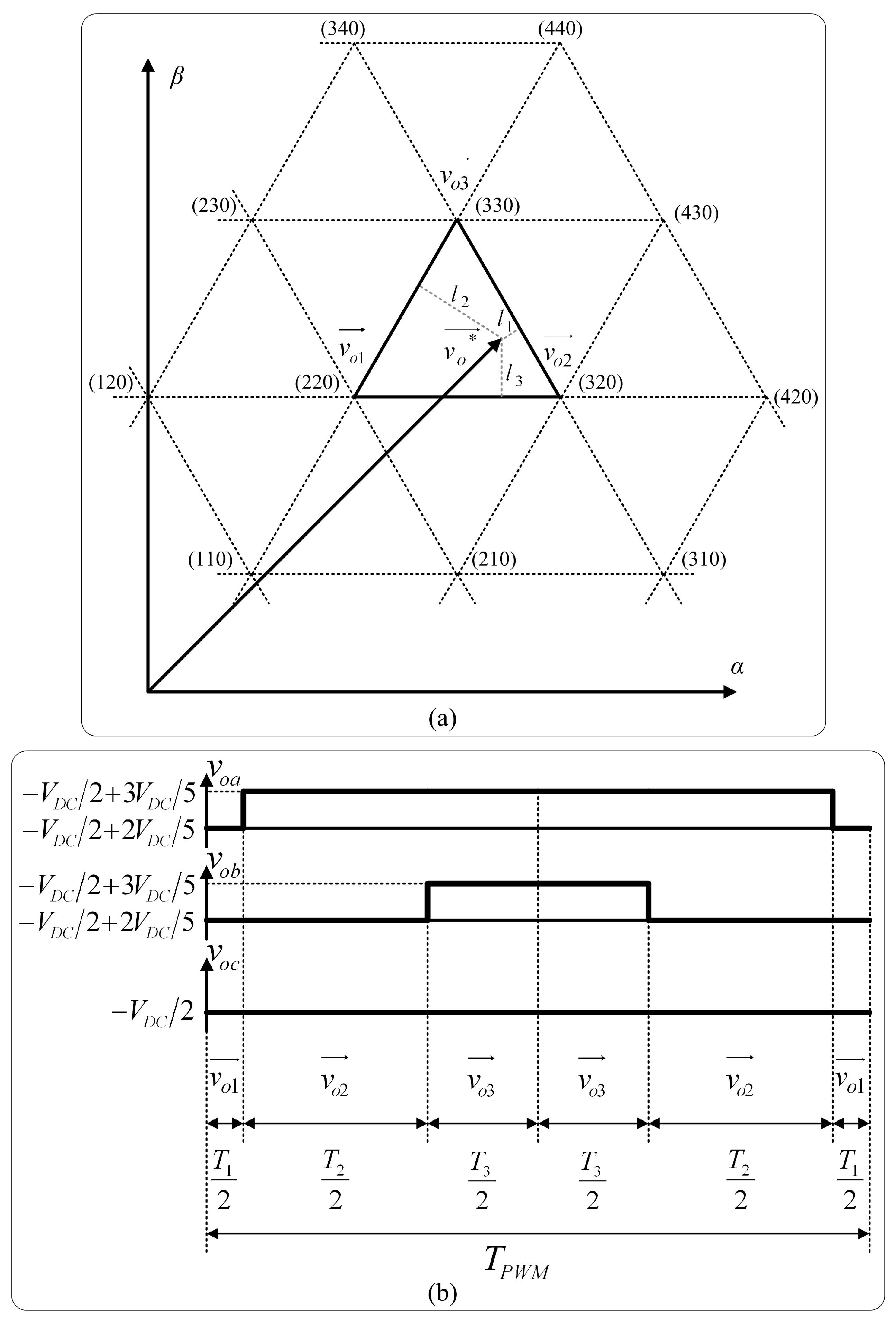
5.1.3. Multilevel SVM

For MMC voltage control, the SVM algorithm can be used in its multilevel version, which has already been used previously for multilevel inverters. In the two-level algorithm, the converter voltage can take eight different values, including nill voltages (000) and (111). The input to the algorithm is the voltage to be generated and the output is three vectors corresponding to inverter voltages, for example (000) (100) (110), and the time each needs to be applied. As the number of levels increases, the number of values that can take the converter voltage grows exponentially, so the selection of the three vectors of the inverter output voltage is more difficult [24,25,26,27,28,29].

Figure 8 presents the basics of the multilevel SVM for the case of six levels. The aim is to generate a reference voltage $\overrightarrow{{v_o}^{*}}$ at the output of the MMC. The voltage values that the converter can generate in an area of the space close to $\overrightarrow{{v_o}^{*}}$ have been represented. The algorithm must be able to determine in which triangle the reference voltage $\overrightarrow{{v_o}^{*}}$ is located and, therefore, which three vectors $\overrightarrow{v_{o1}}$ (220), $\overrightarrow{v_{o2}}$ (320), $\overrightarrow{v_{o3}}$ (330) (Figure 8a) need to be applied to the output voltage of the MMC to generate, by linear combination, the voltage $\overrightarrow{{v_o}^{*}}$. To calculate the application times of each of these vectors ($T_1$, $T_2$, $T_3$) (see Figure 8b), the distances ($l_1$, $l_2$, $l_3$) are calculated in [24] and the times $T_1$, $T_2$, $T_3$ are proportional to these distances. Their sum must be equal to the switching period, $T_{PWM}=T_1+T_2+T_3$.

The output voltage vectors of the MMC $\overrightarrow{v_{o1}}$ (220), $\overrightarrow{v_{o2}}$ (320), $\overrightarrow{v_{o3}}$ (330) correspond to the voltages of the three output phases $v_{oa}$, $v_{ob}$, and $v_{oc}$ whose values can be seen in Figure 8b.

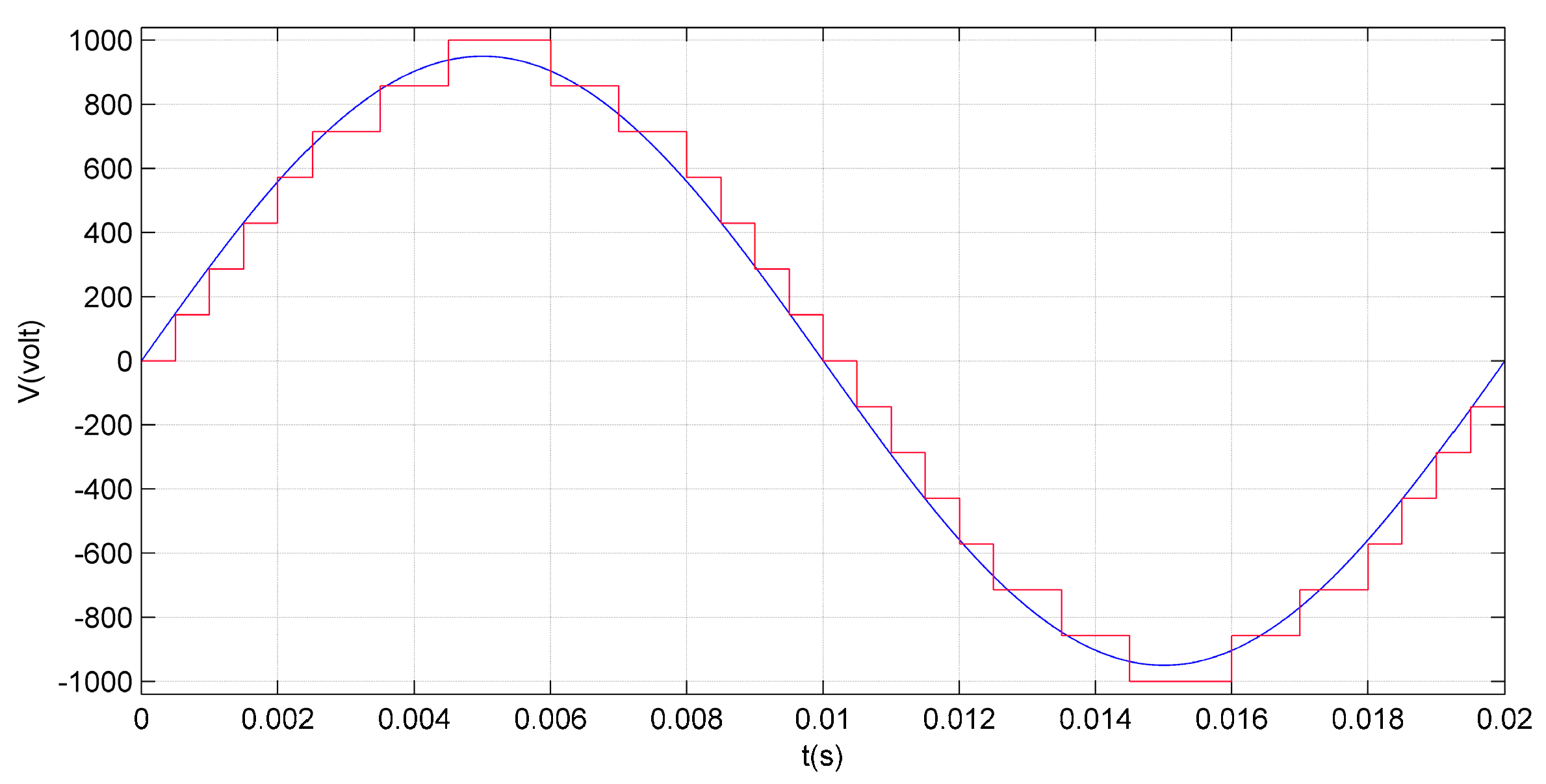
5.1.4. Near Level Control

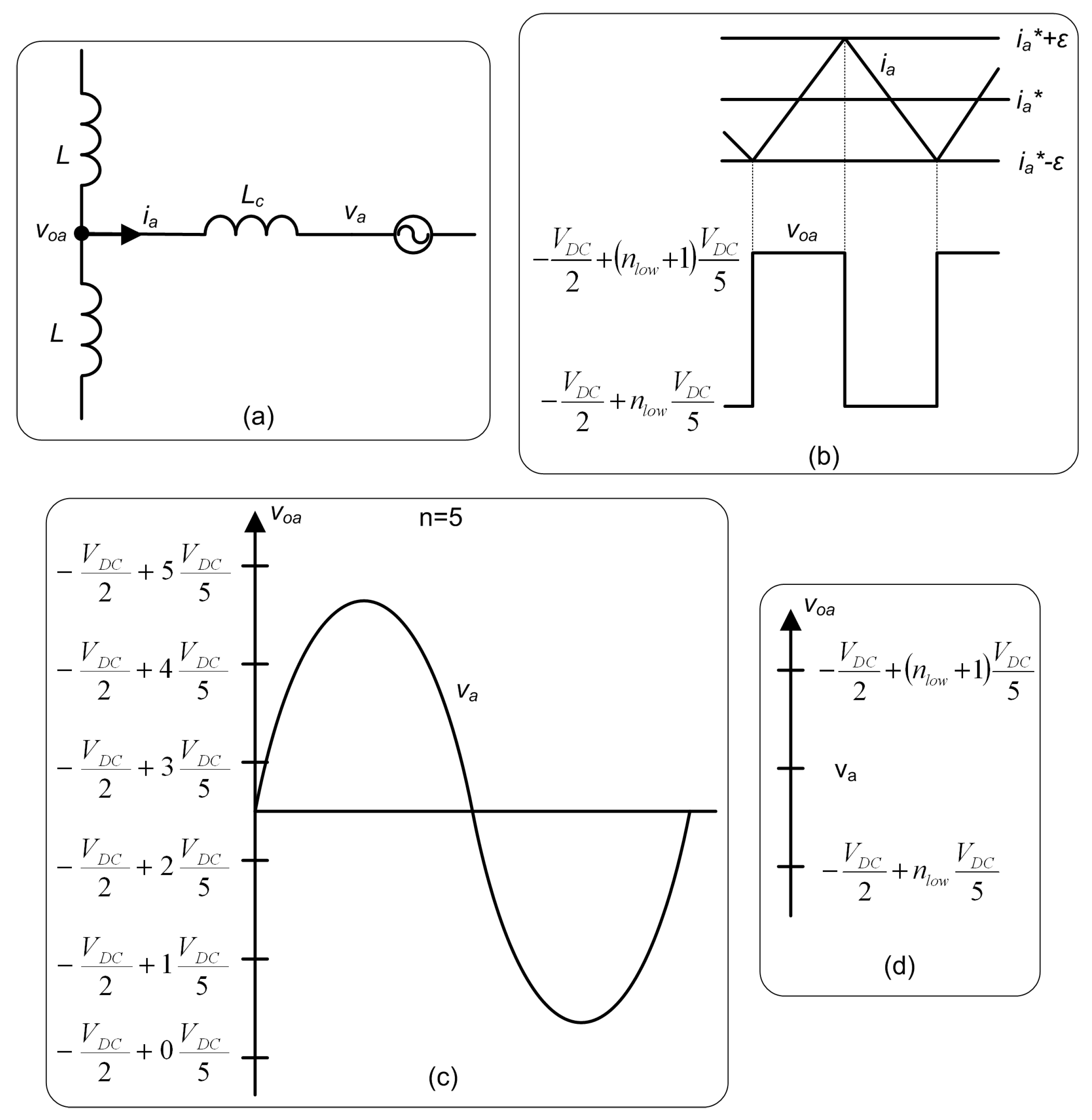
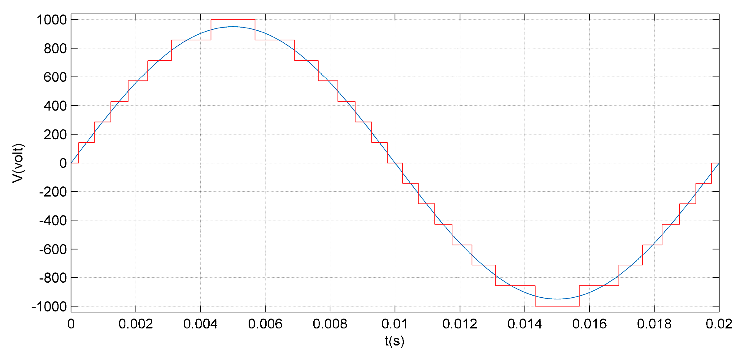
When the number of voltage levels is small, high-frequency modulation is used to generate the voltage. This has the advantage of eliminating the low frequency harmonics and the filtering needs in the AC side, but the disadvantage is the increase of losses by semiconductor switching. If the number of AC voltage levels is high, due to the existence of a large number of SMs per arm, the AC voltage is generated in the form of steps. This causes the semiconductors to have few commutations and low switching losses. The low frequency harmonics are also very small if the number of steps is high and, consequently, the filtering requirements are also small. This output voltage control system is commonly referred to as NLC or sometimes Near Level Modulation (NLM).

NLC can have fixed or variable sampling period $T_s$. In the first case (Figure 9), the variations in the voltage steps occur with a fixed period regardless of the rate of change of the AC voltage [30]. When the number of levels is high, the sampling time must be sufficiently small so that the AC voltage varies only one level at each sampling, not several levels. The control rounds the reference voltage to the values of the available levels.

The second option is for the sampling period to be variable. The control of the switches changes from one level to the next when the reference voltage exceeds the intermediate value at these two levels (Figure 10) [31]. An interesting variation of this method consists in making the upper and lower arms commute out of phase $\frac{T_s}{2}$, causing the number of levels to be multiplied by two [32].

5.2. Current Modulators

The input of the current modulator is the reference of the phase current, which is the output of the PI regulators of the DC voltage $V_{DC}$ and the reactive power $Q$. Current modulators control the MMC output voltage to maintain the current of each phase within a certain hysteresis band. When voltage modulators are used, two additional PI regulators are needed between the current reference and the voltage modulator, which cause the response to be slower than in the case of current modulators. A disadvantage of current modulators is that the switching frequency is not constant, so the design of the filter is more difficult.

The MMC is considered to be coupled to the grid by an inductance (Figure 4), which has, on one side, the output voltage of the MMC $v_{oa}$, and on the other side, the mains voltage $v_a$. By variation of $v_{oa}$, the aim is to maintain the phase current $i_a$ in a band of width $2\epsilon$ around the reference ${i_a}^{*}$. Two current modulators are presented; in the first, the voltage applied to the inductance is constant, while in the second it is proportional to the desired effect [33].

5.2.1. Current Control with Constant Excitation

The coupling inductance has, at the ends, the inverter $v_{oa}$ and grid $v_a$ voltages (Figure 11a). By changing the voltage $v_{oa}$, the current $i_a$ can be maintained within the hysteresis band $\left[\begin{array}{cc}{i_a}^{*}+\epsilon & {i_a}^{*}-\epsilon \end{array}\right]$ (Figure 11b). If the number of SMs per arm is $n=5$, then the voltage $v_{oa}$ can take the six levels observed in Figure 11c, while the voltage $v_a$ will have a sinusoidal form. Although other options may be taken, it seems appropriate to choose the voltages $v_{oa}$ adjacent to the instantaneous value of the voltage $v_a$, $-\frac{V_{DC}}{2}+\left(n_{low}+1\right)\frac{V_{DC}}{5}$, and $-\frac{V_{DC}}{2}+n_{low}\frac{V_{DC}}{5}$ (Figure 11d), where $n_{low}$ is the number of modules in the ON state of the lower arm. When the largest of these values is applied, the voltage at the coupling inductance $L_c$ is positive and the phase current $i_a$ increases (Figure 11b), whereas when the smaller one is applied the opposite occurs. The variable $n_{low}$ is calculated as a function of the grid voltage $v_{oa}$ by the equation:

$$k=floor\left(\left(v_a+\frac{V_{DC}}{2}\right)/v_C\right)$$

(15)

where “floor” means round to an integer towards negative infinity.

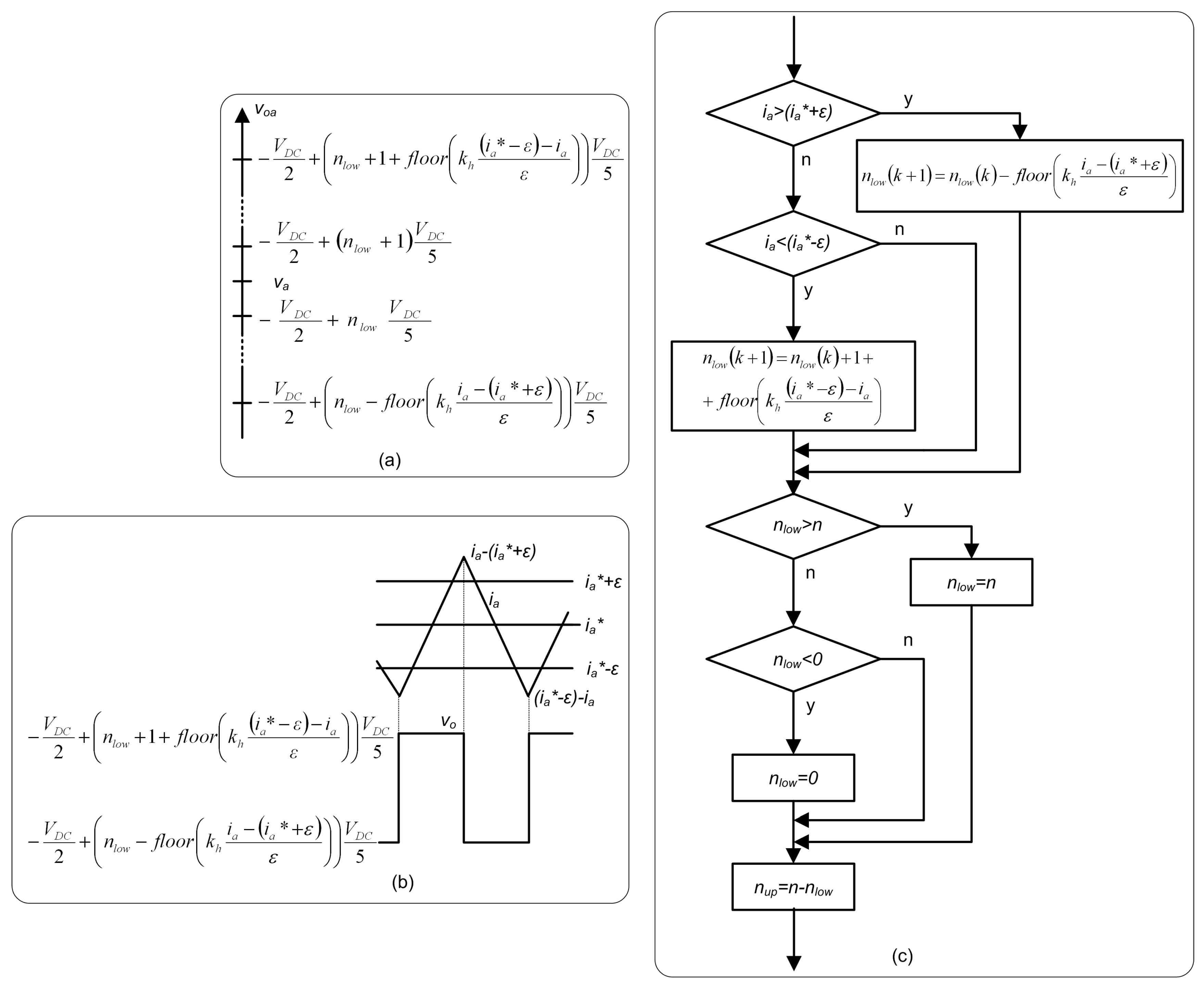
5.2.2. Current Control with Excitation Proportional to the Error

If the number of SMs is very high and the above algorithm is used, the inductance voltage may be too small to be able to direct the phase current $i_a$ in the desired direction; then, a higher voltage is needed. In this case, the values of the MMC voltage $v_{oa}$ adjacent to the grid voltage $v_a$ would not be used, but rather more distant values (Figure 12a) that would cause a faster change of the current $i_a$.

Values of $v_{oa}$ which cause a voltage at the coupling inductance $L_c$ proportional to the distance of the current $i_a$ from the band above $i_a-\left({i_a}^{*}+\epsilon \right)$ or below $\left({i_a}^{*}-\epsilon \right)-i_a$ (Figure 12b) must be chosen. A hysteresis proportionality coefficient $k_h$ is defined which provides greater or lesser voltage in the inductance for the same current error (or distance to the hysteresis band). This coefficient is used in the calculation of the MMC output voltage to be applied when the current goes below the hysteresis band:

$$v_{oa}=-\frac{V_{DC}}{2}+\left(n_{low}+1+floor\left(k_h\frac{\left({i_a}^{*}-\epsilon \right)-i_a}{\epsilon }\right)\right)\frac{V_{DC}}{5}$$

(16)

or above the hysteresis band:

$$v_{oa}=-\frac{V_{DC}}{2}+\left(n_{low}-floor\left(k_h\frac{i_a-\left({i_a}^{*}+\epsilon \right)}{\epsilon }\right)\right)\frac{V_{DC}}{5}$$

(17)

In Figure 12c the current control algorithm diagram with excitation proportional to the error can be seen.

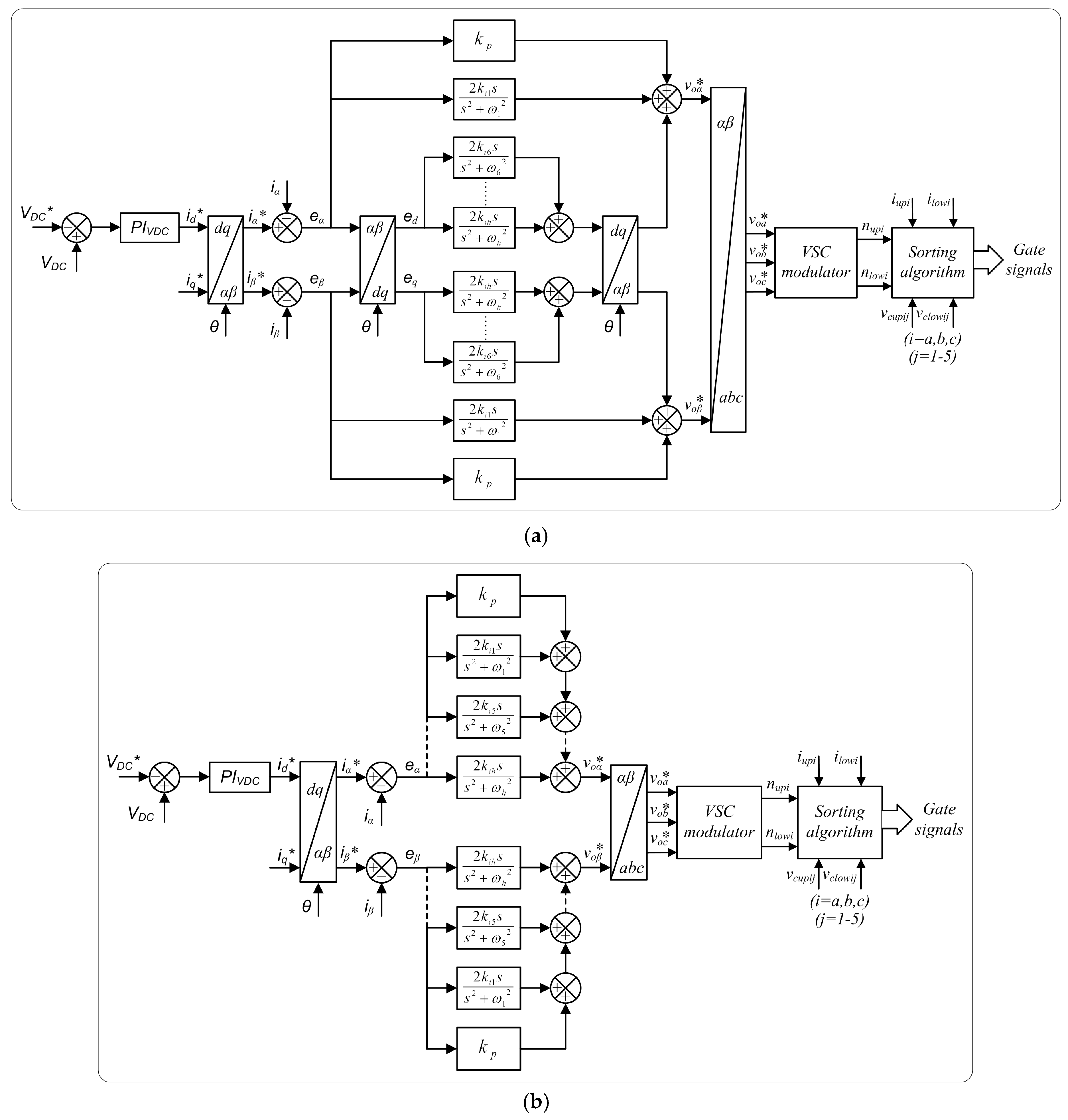
6. Grid Connection

The MMC has one DC side and one AC side. The DC side has a voltage that must be kept constant, either by the MMC or by another converter, depending on the case. The AC side can be a distribution grid (medium voltage) or transport grid (high voltage), or it can be an offshore wind farm.

Usually, the AC part is considered to be a balanced three-phase system containing only the fundamental harmonic. During mains failures, the AC voltage behaves as an unbalanced system, whose unbalance is greater or smaller depending on the distance at which the fault occurred and the type of fault. The grid may also contain harmonics of several frequencies that affect the operation of the converter and the current generated in AC. The following are schemes for controlling MMCs when connecting to balanced, unbalanced, or distorted grids.

6.1. Balanced Grids

When the grid voltage is balanced, the MMC control has external and internal control loops. The external control loop of the MMC can regulate two variables (Figure 13). The first can be the DC voltage $v_{DC}$ or the active power $P$, while the second can be the reactive power $Q$ or the AC voltage $v_{AC}$ [34,35]. The outputs of the external control loops are the grid current references in $dq$ axes, ${i_d}^{*}$ and ${i_q}^{*}$.

The internal control loop may be a current loop (Figure 13a) or a voltage loop (Figure 13b). In the first case, from ${i_d}^{*}$ and ${i_q}^{*}$, the current references of the three phases ${i_a}^{*}$, ${i_b}^{*}$, and ${i_c}^{*}$ are generated, which are the inputs of the current modulator. It calculates the number of SMs in the ON state in each arm $n_{up}$ and $n_{low}$, so the ordering algorithm determines the ON/OFF state of each SM. In the second case, two PI regulators and decoupling equations are used to generate the converter voltage references in the $dq$ axes, ${v_d}^{*}$ and ${v_q}^{*}$.

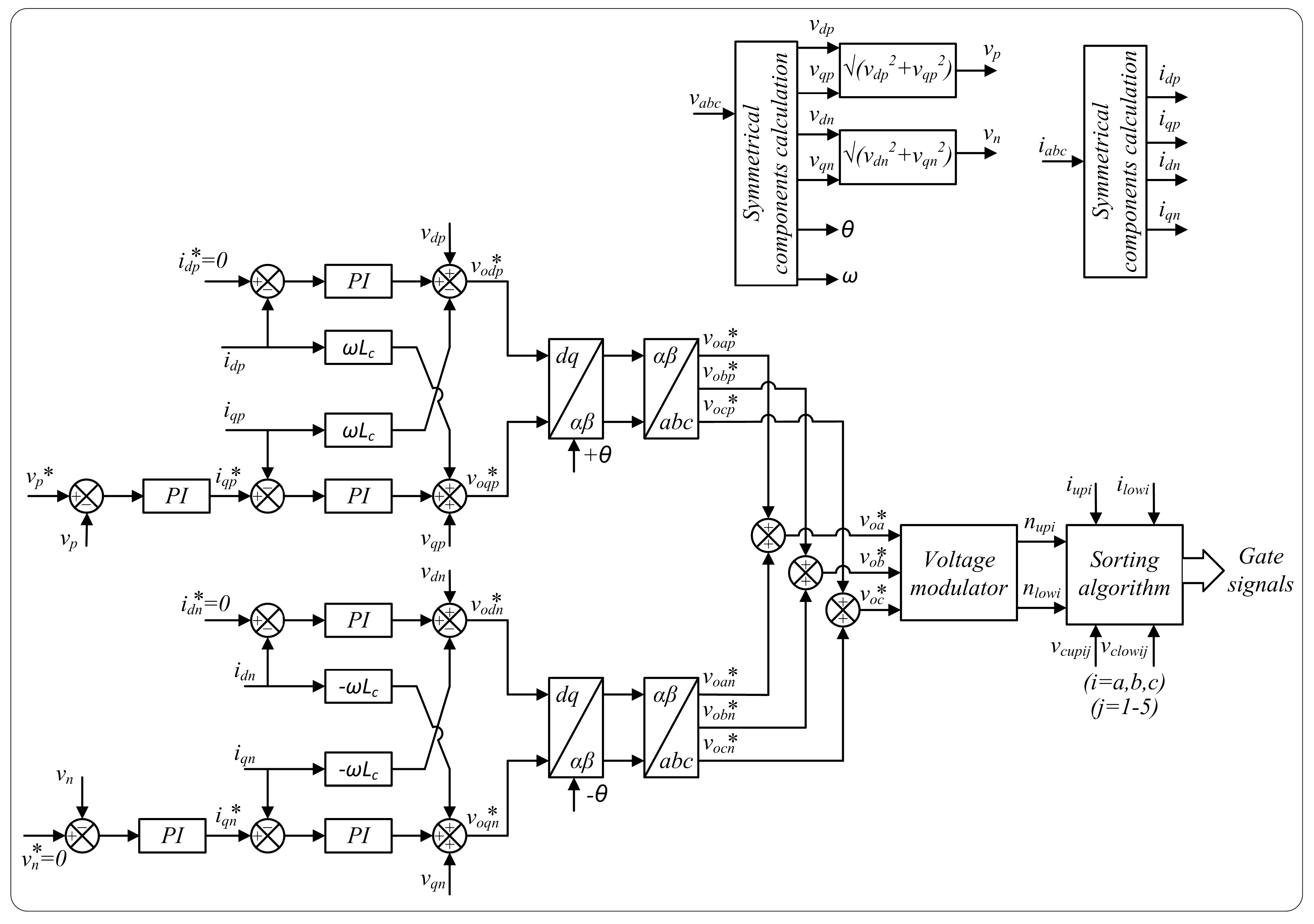
6.2. Unbalanced Grids

When the grid voltage is unbalanced, the positive and negative sequence components must be controlled separately and, finally, the result of each control must be added to obtain the converter reference. According to whether this reference is a current or a voltage, a current or voltage modulator will be used, respectively [36].

Voltage unbalances occur due to grid voltage failures. During them, the grid codes indicate that active power cannot be injected into the grid, and reactive power can only be injected to support the restoration of the grid voltage. Therefore, the control references, both with current modulator (Figure 14) and with voltage modulator (Figure 15), will be:

(1)

For positive sequence, active power $P_p$ must be zero, so the reference of the positive sequence current on the $d$ axis must be zero, ${i_{dp}}^{*}=0$.

(2)

A PI regulator is used to try to reset the positive sequence grid voltage to its nominal value ${v_p}^{*}$, by the action of the positive sequence reactive power $Q_p$, which is controlled by the positive sequence current in the $q$ axis, ${i_{qp}}^{*}$.

(3)

For the negative sequence, the active power $P_n$ must be zero, so the reference of the negative sequence current on the $d$ axis must be zero, ${i_{dn}}^{*}=0$.

(4)

A PI regulator is used to try to establish the negative-sequence grid voltage to zero, ${v_n}^{*}=0$, by the action of the negative sequence reactive power $Q_n$, which is controlled by the negative sequence current on the $q$ axis, ${i_{qn}}^{*}$.

It is necessary to use an algorithm that calculates the positive and negative sequence components of the grid voltages and currents (the latter only for the case of a voltage modulator), as well as the angle $\theta$ of the positive sequence $dq$ reference. An algorithm very usually used is the so called Delayed Signal Cancellation (DSC) [37,38].

When a current modulator is used, the references of the positive (${i_{ap}}^{*}$, ${i_{bp}}^{*}$, ${i_{cp}}^{*}$) and negative (${i_{an}}^{*}$, ${i_{bn}}^{*}$, ${i_{cn}}^{*}$) sequences are added to obtain the current reference of each phase (${i_a}^{*}$, ${i_b}^{*}$, ${i_c}^{*}$) (Figure 14). When a voltage modulator is used, current references must be converted to voltage references, for positive and negative sequences, by two PI regulators and axis decoupling equations. Finally, the voltage references of the three-phases, for positive (${v_{oap}}^{*}$, ${v_{obp}}^{*}$, ${v_{ocp}}^{*}$) and negative (${v_{oan}}^{*}$, ${v_{obn}}^{*}$, ${v_{ocn}}^{*}$) sequences, are added to obtain the voltage reference of each phase (${v_a}^{*}$, ${v_b}^{*}$, ${v_c}^{*}$).

6.3. Distorted Grids

In a 3-phase grid-connected system with two degrees of freedom (three wire connection), and the utility grid voltages with fundamental frequency ${\omega }_1$ and harmonics at $\left(6n\pm 1\right){\omega }_1$, $n=1,2,3,4,\dots$, it is mandatory to implement a control strategy for the inner current loop that must be able to track the fundamental frequency ${\omega }_1$ of the reference signal command and reject the harmonic perturbations in order to attain a zero steady-state error.

When the sequence of the fundamental frequency is positive/negative, it is well-known that the sequence of the harmonics $5{\omega }_1$, $11{\omega }_1$, $17{\omega }_1$, etc., will be negative/positive, meanwhile the sequence for the $7{\omega }_1$, $13{\omega }_1$, $19{\omega }_1$, etc., ones will be positive/negative. In addition, knowing that this system has two degrees of freedom, it can be transformed into a 2-phase system in the orthonormal $dq$ and $\alpha \beta$ axes so as to be able to exert a decoupled control of the instantaneous active and reactive powers [39]. Then, the $dq$ components of the output currents ($i_d$, $i_q$) will have the $6n{\omega }_1$ harmonics, $n=0,1,2,3,4,\dots$, while the $\alpha \beta$ components ($i_{\alpha }$, $i_{\beta }$) will have the same fundamental frequency ${\omega }_1$ and its harmonics at $\left(6n\pm 1\right){\omega }_1$, $n=1,2,3,4,\dots$ [40].

According to the internal model principle (see Appendix C of [41]), and when the poles of the closed-loop transfer function are in the left-half of the complex plane (stable system), a PI regulator can only track DC reference signals and reject DC perturbations, while a Proportional-Resonant (PR) regulator can track and reject sinusoidal signals with frequency $\pm {\omega }_o$, that is, of both positive and negative sequence, if the resonant part of the PR regulator is tuned to ${\omega }_o$. If the current control is exerted in the $dq$ axes using two PI regulators, the harmonic perturbations $6n{\omega }_1$ ($n=1,2,3,4,\dots$) cannot be cancelled unless a feedforward scheme for the cross-coupling terms and the utility grid voltage are used; but the feedforward scheme will work properly if the switching frequency of the MMC is high enough to allow a higher controller bandwidth to avoid the delay effects. Consequently, the cost of the electronic conditioner circuit will be increased and the use of a powerful microcontroller will also be mandatory.

To deal with the restrictions of PI regulators mentioned above, several strategies can be used to implement the inner current controller based on selective harmonic compensation schemes and using low-cost commercial microcontrollers [42]. Among them, two strategies capable of tracking sinusoidal reference signals and cancelling sinusoidal perturbations are explained below. Both strategies employ resonant filters tuned at the frequencies to be compensated:

(1)

Control in $\alpha \beta -dq$ axes: In this control, PR regulators are applied to the current errors in $\alpha \beta$ axes ($e\alpha \beta$) to track the fundamental reference signal, while the compensation of the harmonics $6n{\omega }_1$ ($n=1,2,3,4,\dots$) is exerted on the current errors in the $dq$ axes ($edq$, where the $\alpha \beta \to dq$ transformation is applied), cascading several resonant filters tuned to these harmonic frequencies. After the application of the inverse transform $dq\to \alpha \beta$, all the $\alpha \beta$ signals are added to obtain the reference output voltages (${v_{o\alpha }}^{*}$, ${v_{o\beta }}^{*}$) to feed the VSC modulator [43] (see Figure 16a).

(2)

Control in $\alpha \beta$ axes: For this, two PR regulators are used for the current errors ($e\alpha \beta$) to track the reference signal with the fundamental frequency ${\omega }_1$, and several resonant filters tuned to the harmonics to be compensated $\left(6n\pm 1\right){\omega }_1$, $n=1,2,3,4,\dots$, are cascaded in each axis. The output of both the PR regulators and the resonant filters in the $\alpha \beta$ axes are added to obtain the reference output voltages (${v_{o\alpha }}^{*}$, ${v_{o\beta }}^{*}$) needed to feed the VSC modulator [44,45] (see Figure 16b).

Finally, it is worth noting that the above strategies have a similar performance regarding their harmonic compensation capability. So, the ease of implementation, together with the execution time of the corresponding discrete algorithms, will lead to the best solution [42].

7. Applications

The main application of the MMC is HVDC transmission, although it has also been used in other applications such as the distribution static synchronous compensator (D-STATCOM) and low voltage inverter.

7.1. HVDC

The converter topologies used in HVDC were LCC first and later VSC. MMCs are currently being used, and they are being installed by major power companies such as Siemens [16], ABB [46] or Alstom [47]. HVDCs are used for the interconnection of high voltage AC grids and the connection of offshore wind farms to land (the latter subject will be looked at later).

Table 3. Projects using modular multilevel converter (MMC) technology.

Project	Year	Power (MW)	DC (kV)	AC (kV)	Application	Manufacturers
Trans Bay Cable	2010	400	±200	230	Grid connection	Siemens
COBRAcable	2019	700	±320	400	Grid connection	Siemens
North Sea Link	2021	1400	±525	Kvilldal: 420 Blyth: 400	Grid connection	ABB
Caithness Moray	2018	1200	±320	Spittal: 275 Blackhillock: 400	Grid connection	ABB
BorWin1	2011	400	±150	Platform BorWin Alpha: 170 Diele: 380	Offshore wind farm	ABB
BorWin2	2015	800	±300	Onshore: 380 Offshore: 155	Offshore wind farm	Siemens
BorWin3	2019	900	±320	-	Offshore wind farm	Siemens
DolWin1	2015	800	±320	Dörpen West: 380 Dolwin Alpha: 155	Offshore wind farm	ABB
DolWin2	2016	916	±320	Dörpen West: 380 DolWin Beta: 155	Offshore wind farm	ABB
DolWin3	2017	900	±320	-	Offshore wind farm	GE-Alstom
HelWin1	2015	576	±250	Onshore: 380 Offshore: 155	Offshore wind farm	Siemens
HelWin2	2015	690	±320	400	Offshore wind farm	Siemens
SylWin1	2015	864	±320	400	Offshore wind farm	Siemens
ULTRANET	2019	2000	±380	400	Grid connection	Siemens
INELFE	2015	2000	±320	400	Grid connection	Siemens
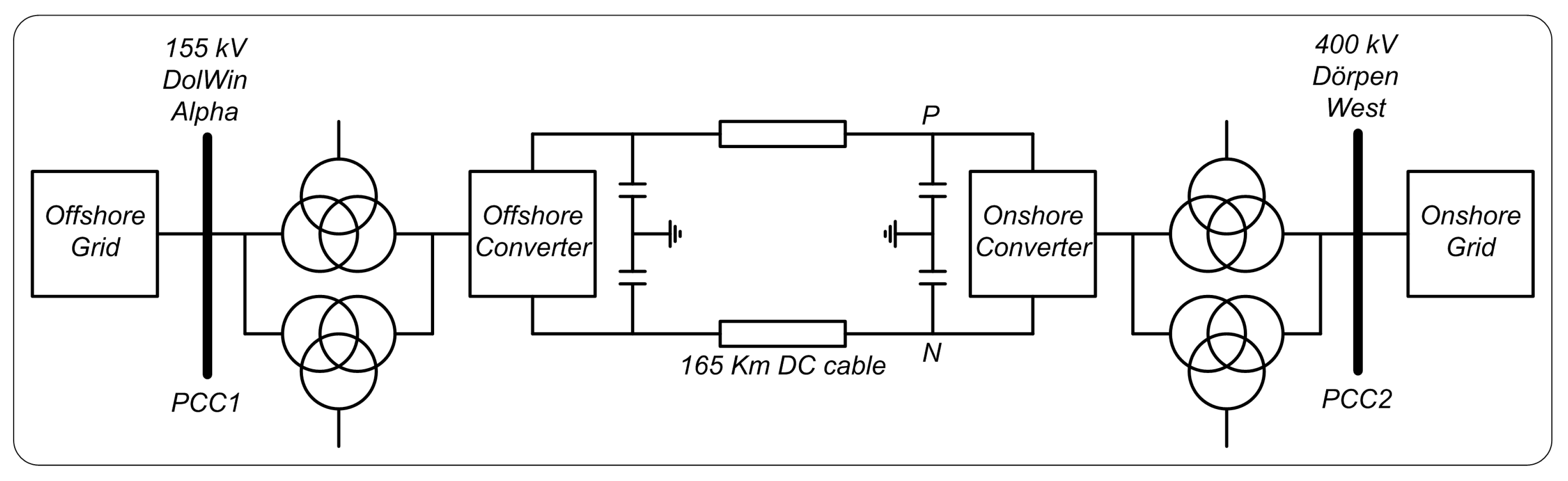
Skagerrak Pole4	2014	700	±500	700	Grid connection	ABB

shows some of the projects that use MMC technology, including Trans Bay Cable, which was the first HVDC project to use MMC. Most converters use a topology with a large number of cascaded HB-SMs in a symmetrical monopolar configuration. The vast majority of offshore applications created or planned in recent years have been in Germany, linked to the creation of numerous offshore wind farms. For an HVDC voltage level of ±320 kV, as in DolWin1 (Figure 17), n = 38 HF-SM (formed by IGBT) per arm are usually required. Each SM switches to a low frequency of approximately 150 Hz so the losses are small, but the stepwise switching of the SMs makes the effective frequency per phase greater than 10 kHz, greatly reducing the filtering needs in AC.

The connection of AC grids through HVDC occurs in several circumstances:

(1)

Connection of different frequency grids (50 and 60 Hz).

(2)

Connecting asynchronous grids.

(3)

Connecting islands with the mainland.

(4)

Connection of continental grids that have less distance by sea than by land.

(5)

Connection of weak grids in which the converters provide grid support service by reactive power injection.

7.2. D-STATCOM

Medium voltage distribution lines frequently have problems of reactive compensation, voltage variations, unbalances, and harmonics. Voltage variations occur in weak lines due to the starting or stopping of large motors or to load excess/defect. The unbalances are due to the application of single-phase loads and asymmetric faults. The harmonics are motivated by the presence of nonlinear loads and the saturation of transformers. The D-STATCOM is used to improve this situation through its great capacity for reactive compensation and voltage regulation.

The H-bridge topology has usually been used for D-STATCOM due to the ease of obtaining a high number of levels, but it has limitations in situations of load or network unbalances. Therefore, solutions based on MMC have been proposed as they have more degrees of freedom to carry out the control and greater capacity of power [48,49].

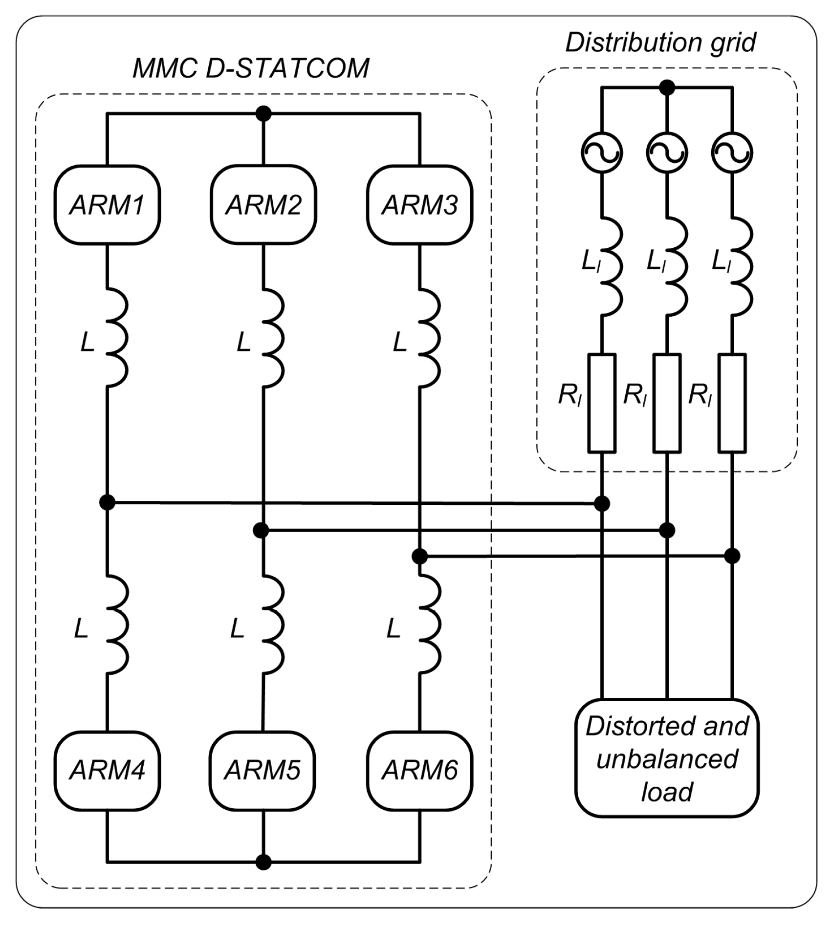
The use of an MMC with a large number of levels allows coupling to the grid without the need of a transformer (Figure 18). An external capacitor that maintains the DC voltage is not necessary, as that function is carried out by SM capacitors. An interesting concrete application for the MMC-based D-STATCOM could be the improvement of power quality in railway traction systems.

7.3. Low Voltage Multi-Level Inverter

MMCs have been used in low voltage DC (LVDC) applications and generator drives. Some applications such as electrical supply, recharging of electric vehicles, and aerospace require high levels of performance, power quality, and electro-magnetic interference (EMI). They can be achieved by MMCs made with silicon carbide metal-oxide semiconductor field-effect transistor (SiC MOSFET) and Si MOSFET [50]. The use of MOSFET instead of IGBT is able to reduce switching losses, while the use of synchronous rectification reduces conduction losses [51]. In [52], an MMC has been used as an interface with the power grid of a Smart Home that includes photovoltaic generation, energy storage, and recharging of electric vehicle, all connected to a DC bus. The MOSFET MMC topology has been compared with the classic multilevel topologies, with advantages such as filter reduction, simpler redundancy, and reduced power losses, making it a more appropriate topology for Smart Homes.

In [53], an MMC has been used as AC/DC converter to control a wind generator without gear box. Multilevel converters are suitable for this application because of their lower harmonic content, as well as the reduction of semiconductor stress and electromagnetic disturbances. MMC has such advantages over classical multilevel topologies as its modular design, simple structure, ease of increasing the number of levels, faster replacement of faulty modules, and reduced number of semiconductors.

8. Integration of Offshore Wind Farms

8.1. Global Control of the HVDC MMC

In an HVDC system, the control of each converter interacts with the other, although they are different [36,54]. Whereas the grid side MMC has to keep the DC voltage within a range of values, the wind farm side MMC has to get the maximum power from the wind park, where other electronic converters take the wind turbines to the optimum operation points for each type of wind.

There are two possibilities to implement the control of an HVDC system: using or not using communications. Using communications is the preferable solution in multiterminal HVDC networks because it enables complex coordinated control systems to carry out the necessary tasks, taking into account a number of voltages and currents.

In point to point topology, a simpler control strategy, with no communications, can be chosen; this can be used even with multiterminal topologies [54]. In this strategy, the control of the grid side MMC is based on a droop technique: as the DC voltage increases, the electric current injected into the grid also increases, so as to keep the voltage within a range of values. The limit is the semiconductors rated current.

The control of the wind park side MMC works by extracting the whole electric power generated by the wind farm for every wind speed, within two limits: the semiconductor rated current and the maximum DC bus voltage. The former cannot be exceeded in any case, whereas the latter forces the current taken from the wind park to reduce progressively once a certain limit of DC voltage is reached, once again using a droop based technique.

8.2. Power Collection in Wind Farms

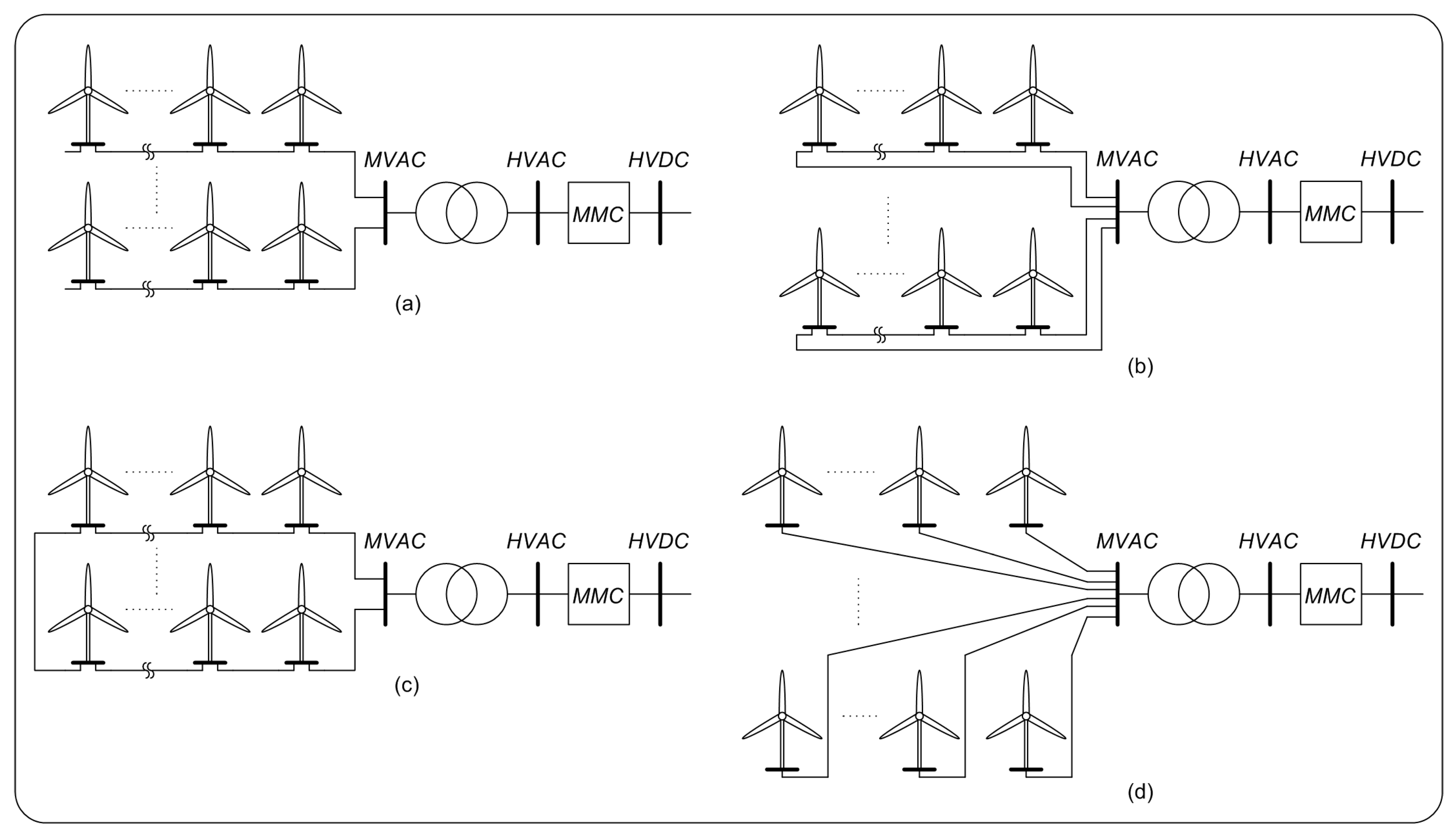
The electric circuit used in wind farms to collect the energy generated by wind turbines comprises several feeders connected to a MV hub in several possible configurations. Also, wind generators are often connected to each other to form a string. The whole system is known as a collection system. A number of collection systems have been proposed in the technical literature for offshore applications, making use of different wind generator arrangements, such as radial, single-sided ring, double-sided ring, star, etc.

8.2.1. Radial Arrangement

This configuration, Figure 19a is the simplest possible arrangement of wind generators. In this set up, the wind generators within the same feeder are connected in series, making up a string. The maximum number of generators that can be connected to each feeder depends on the submarine cable cross-section and the generators’ rated power. The main advantage is the low cost, while the main drawback comes from the fact that, if a generator close to the MV hub fails, the whole string is disconnected, losing the power generated by all the generators that make up the string [55,56].

8.2.2. Single-Sided Ring Arrangement

By using an additional cable run, an extra security measure can be added to the radial setup at the expense of a long return cable of a large cross-section, capable of transporting all the electric power generated in the string, Figure 19b. The new cable connects the outermost wind generator to the MV hub. In case of a cable failure, or when a circuit breaker opens the ring, the electric power generated in the rest of the wind turbines can be transported to the MV hub using the return cable.

8.2.3. Double-Sided Ring Arrangement

In this configuration, Figure 19c, the last wind generator belonging to a string is connected to the last wind generator of the next string. In case of a cable failure, or when the string is opened by a circuit breaker, the total power generated by the remaining connected generators has to be transported through the other string to the MV hub. In consequence, the rated current of both cable strings must be oversized to allow bidirectional power flow in case of cable failure [55,56,57].

The redundancy feature provided by ring configurations makes sense, particularly in offshore installations, where the repair downtimes are significantly longer when compared to those onshore and the repair costs are much higher.

8.2.4. Star Arrangement

This configuration, Figure 19d, is intended to reduce the cable ratings and provide the wind farm with high reliability (in case of a cable failure, only one wind generator is lost). The most important drawback is the complex switchgear requirement at the center of the star [55,56,57].

All the aforementioned AC collection systems use utility frequency transformers on the off-shore transmission platform. This might be a drawback, since they are big, heavy, and require a large support structure, which entails a high transport and installation cost. AC collection systems also need reactive power compensation devices and power quality filters, which take up a lot of space on the offshore platform [58].

New developments are taking DC collector systems into consideration in wind and wave farms [58,59,60]. They present some advantages, such as needing less space for the DC cables on the platform and a lower weight than for those of the equivalent AC cables; in addition, they do not need reactors for reactive power compensation either. The intermediate DC link also decouples the wind farm from the mainland grid, thus increasing the capability of the wind turbines to withstand faults. However, DC collector systems, as well as AC systems, present some drawbacks, such as, for example, DC protection is still expensive.

9. Conclusions

MMC technology has shifted towards the classical topologies of LCC and VSC, and has been established as a preferred solution for carrying out HVDC links by the main installation companies. It has also been proposed, however, as a solution for the realization of multilevel converters in MV and LV. The most important high voltage applications are the connection of electric energy transport grids and the connection of large offshore wind farms to the terrestrial grid. The increase of its implantation in applications of MV and LV is predictable in the future, due to its good characteristics.

Although the topology commonly used for SMs is HB, it does not have the capability to reduce DC short-circuits. The FB topology, also used by the manufacturers, has the ability to eliminate DC faults, with other topologies that can be used for this purpose. This will become of great importance in the future when building multi-terminal HVDC grids.

For the correct operation of MMC, the capacitor voltage of the SMs must remain constant. The capacitors can be charged or discharged by arm currents, by turning ON the appropriate SM. The most commonly used balancing method was explained in detail. Other methods that can be found in the literature were briefly presented.

The voltage or current modulators are responsible for making the voltage or current of the converter follow their references. Four voltage modulators and two current modulators were presented in detail. The former are more commonly used because they require a lower switching frequency and allow the design of the AC filter to be simpler. The latter have been proposed for applications in which the speed of response is more important.

The external loop regulates DC link voltage and reactive power, using voltage control or current control schemes. When imbalances occur, the regulation prevents the injection of active power and allows the injection of reactive power to help restore the mains voltage. The low order harmonics of the mains voltages will be introduced into the internal current loop in the form of disturbances, distorting the output currents. To avoid this, proportional-resonant regulators tuned to the frequency of the fundamental, as well as to the frequencies of the harmonics (or their equivalents in dq axes) have been proposed.

The most important application of the MMC is in HVDC transmission, to make marine connections (land to land, wind farm to land), and the interconnection of different frequency grids and asynchronous grids. Other applications of MV and LV were also presented. In the future, it is expected that MMC will be the technology used in new HVDC installations, that it will greatly increase its presence in commercial MV applications, and that it will increase its presence in LV applications at the research level.

A very important application is the connection of offshore wind farms to the transmission grid. End stations can be synchronized using communication systems or work independently following specific rules. In the future, research on how to connect individual turbines and turbine groups to obtain HVDC is foreseeable.

As the penetration of the HVDC transmission increases, the need for research on multi-terminal grid connection, oriented to the control of load flow and to the protection against faults, will increase.