Abstract
This paper proposes a novel min-max control scheme for aircraft engines, with the aim of transferring a set of regulated outputs between two set-points, while ensuring a set of auxiliary outputs remain within prescribed constraints. In view of this, an optimal augmented monotonic tracking controller (OAMTC) is proposed, by considering a linear plant with input integration, to enhance the ability of the control system to reject uncertainty in system parameters and ensure no crossing limits. The key idea is to use the eigenvalue and eigenvector placement method and genetic algorithms to shape the output responses. The approach is validated by numerical simulation. The results show that the designed OAMTC controller can achieve a satisfactory dynamic and steady performance and keep the auxiliary outputs within constraints in the transient regime.
1. Introduction
In many practical control problems, some actuators are employed to control corresponding outputs of interest (called main outputs), while a set of remaining outputs (called auxiliary outputs) must keep within prescribed ranges in a non-square system where the number of outputs is larger than that of inputs. In aircraft engine control, rotor speed is the primary regulated variable, while the outputs such as turbine temperatures and compressor pressures must be kept within limits. There are three circumstances that can cause limits to be exceeded, i.e., steady limit violation, transient violation and off-nominality. Steady limit violations tend to ensue at steady state if the regulated variable is driven to a set-point outside the permissible constraints. Transient violations mean that auxiliary outputs have exceeded the limits during transition. Off-nominality may result from a change in controller tuning to address new performance requirements for the regulated variable or from unintentional factors such as plant parameter variations or external disturbances [1]. In recent decades, numerous studies concerning limit management have been carried out to prevent the outputs of aircraft engines from exceeding their corresponding limits. Min-max arrangement is a representative method of aircraft engine control systems for the realization of limit management. Since this method was introduced, the research on how to improve its limit protection ability has been an academic focus [2,3,4,5,6]. The authors of [2] used conditionally active limit regulators in the min-max architecture. In [3], an emergency control law was designed for nonlinear engines with uncertain dynamics due to off-nominal operation. In [4,5,6], Richter et al. proposed the use of sliding mode control or model predictive control in aircraft engine limit management.
It should be noted that when a min-max control selection structure is employed, its regulator will take over and attempt to drive the output to the prescribed limit, if one auxiliary output approaches its limit. The multi-regulator scheme with integral control and min-max selectors is shown in Figure 1. The regulators provide control input rates. Let and . stands for the steady state when the output tracks , where . Thus, the min-max selection law is expressed as:
where are the min-selected regulator outputs and are the max-selected regulator outputs.
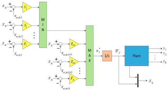
Figure 1.
Min-max multi-regulator system with integral control.
As we know, auxiliary outputs may display overshoots and undershoots as the main output is controlled to a set-point [7]. In a sense, the standard min-max arrangement may be ill-conceived when used in conjunction with linear regulators, because there is no way to guarantee that one auxiliary output can be driven to the prescribed limit without overshoot. Thus, the idea of decreasing or even eliminating the overshoots and undershoots may be feasible to implement limit management. In recent years, a method was designed to avoid overshoot for linear time invariant (LTI) systems [8]. This method, employing the classic eigenstructure assignment algorithm of [9], can achieve arbitrarily fast settling times while guaranteeing a non-overshooting response in all components of the output vector for any initial condition. A modified approach is developed to prevent the step response from undershoot [10]. For sake of ensuring monotonic tracking, a necessary and sufficient structure condition is developed by using a geometric approach [11]. In [12], a computationally tractable necessary and sufficient LMI condition was offered to obtain a characterization of monotonicity in terms of the left eigenvectors of state transition matrix. A common feature of these papers above is to design a tracking controller for system whose number of outputs is less than or equal to that of input, but for system whose number of outputs is more than that of inputs, the auxiliary outputs may not be shaped with monotonicity when the main outputs track a reference.
In this paper, a novel method is developed to formulate a state feedback tracking controller for improving min-max limit protection in aircraft engine control. The key idea of this method is that the transient response of the system outputs is shaped in advance for obtaining generalized monotonicity by using the eigenvalue and eigenvector placement method and genetic algorithms, to avoid the occurrence of overshoot and undershoot so that auxiliary outputs will remain within their prescribed bounds in the transient regime. An augmented approach using integral control is applied to obtain robust tracking for resisting the uncertainties in the plant parameters which cause the tracking error to be nonzero.
2. State Feedback Controller Design Method
In this section, we discuss an augmented monotonic tracking controller applied for a non-square system with prescribed output constraints. To enhance robustness, a linear time-invariant system with input integration is considered.
2.1. Augmented Monotonic Tracking Controllers
Consider the linear time-invariant system:
where, for all , is the state, is the control input, is the output, and , , and are appropriate dimensional constant matrices. Assume that has full column rank and has full row rank. In this paper, the aircraft engine state variable model (SVM) in Equation (2) is extracted by using the Commercial Modular Aero-Propulsion System Simulation (CMAPSS). CMAPSS is a Simulink port and a database with a user-friendly graphical user interface (GUI) allowing the user to perform model extraction, elementary control design, and simulations without much effort [13]. The linearization method used in CMAPSS for establishing engine SVM is a bias derivative method; for details, readers may refer to [14].
As aircraft engines are often considered to be a single-input and multi-outputs plant, system may be non-square. Then we decompose system into two components: square system and system , which are governed by:
where is a square system with main outputs to be tracked and is a system with the constrained auxiliary outputs . The output vector and appropriate dimensional constant matrices and of system can be represented as:
where stands for the output of system , and denote the row vector of the output matrix and , respectively.
As we know, the monotonic tracking controller will result in zero steady-state error to a step reference for linear system with no uncertainty [8], but in most real cases there are always some uncertainties in the plant parameters which cause the tracking error to be nonzero, and reduce the tracking accuracy of state feedback law for aircraft engines. One practicable method is to use integral control to obtain robust tracking. Then the ability to track references and reject uncertainties of the control system can be enhanced. To achieve integral control, the following augmented plant can be described as:
where , , is the new control input which equals to and the augmented state vector and system matrices are defined as:
The number of system outputs is:
The order of the system is:
First, following assumptions are necessary to be adopted to design a monotonic tracking controller for system .
Assumption 1.
System is right invertible and stabilizable, and has no invariant zeros at the origin.
Assumption 2.
System is square.
Assumption 3.
System has at least distinct invariant zeros in .
Next, the relationship between the invariant zeros of system and system is discussed.
Theorem 1.
The invariant zeros of system is same as that of augmented system .
Proof.
Let denote the set of distinct invariant zeros of system . Then, the rank of the system matrix pencil drops from its normal value for . The system matrix pencil of system is given by:
where and are the matrices formed by , and , which can be expressed as:
where , , and are appropriate dimensional identity matrices. Properties of matrix elementary transformation implies . Hence, the invariant zeros of system and are the same.□
For definiteness and without loss of generality, Assumption 3 is replaced by the following Assumption 4:
Assumption 4.
System has at least distinct invariant zeros in .
The following method is developed to design a tracking controller such that is stable for a step reference signal with state feedback gain matrix . Let and denote the control input and the state at steady state, respectively. Then:
for any step reference , where and is obtained by solving the following equation:
Let the tracking error vector and suppositional tracking error vector be defined as and , respectively, where suppositional tracking reference is defined as . Applying the state feedback control law:
to Equation (5) and employing the change of variable , we obtain the closed-loop autonomous system:
Since is stable, converges to , converges to and converges to as goes to infinity.
Definition 1.
If the main output and the auxiliary output obtained from applying in Equation (13) are all monotonic, then we define this property as generalized monotonicity.
The following is the specific design method to shape the responses of the main output and auxiliary outputs. The key idea is the choice of a suitable closed loop eigenstructure, which is composed of eigenvalues and eigenvectors such that generalized monotonicity can be achieved. Firstly, decompose the set into two parts. One part is the set of distinct invariant zeros composed of for . Another part is the set composed of for , which may be freely chosen to be any distinct real stable modes. To obtain , let be such that:
where is the canonical basis of . Provided is linearly independent, then sets and are obtained by solving the Rosenbrook matrix equation:
for . The sets , and all meet the requirements of Proposition 1 in [13], then a gain matrix can be obtained by use of the procedure given in that paper such that has the desired eigenstructure. It is worth noting that when is real, , where and . Since , the vectors in satisfy:
Notation 1.
For each , let:
- (1)
- and denote the eigenvectors in associated with canonical basis vector in Equation (15), and let and be the eigenvalues corresponding to and , ordered such that in each case;
- (2)
- Let be the coordinate vector of in terms of . Then define:
Theorem 2.
Assume that Assumptions 1, 2, and 4 are all satisfied. Let be a set of desired closed-loop poles, and assume that the set of associated eigenvectors obtained from solving Equation (16) with in Equation (15) is linearly independent. Let and be any step reference and any initial condition, respectively. Then, the output obtained from applying in Equation (13) to tracks monotonically if and only if for all .
Proof.
The tracking error vector can be expressed as:
Define:
Then:
Let:
(Sufficiency). If , then the following two possible situations should take into consideration:
If condition 1 holds, increases monotonically with increasing and takes its minimum value at . The sign of is determined by the sign of as is a positive constant. Then, we have , which yields for all . It means that the feature of monotonicity of is kept. Thus, the component of the output tracks monotonically. The proof of condition 2 and condition 1 are similar. (Necessity). If , we will concern about the following four possible situations:
If condition 1 holds, we have . In order to keep the sign of unchanged, only need to let the condition hold as increases monotonically with the increasing . The proof of condition 2 is similar to condition 1. If condition 3 holds, then . Thus, in either case does not change sign. The proof of condition 4 is similar to condition 3.
It can be known that the output converges to monotonically if and only if for all .
After obtaining the condition of how to achieve the monotonicity of , then we think about how to keep the output monotonic in order to obtain generalized monotonicity. The suppositional tracking error vector is defined as:
where is the row vector of , for , and for . Then, for and for can be given by Equations (26) and (27), respectively. Then:
In Equations (26) and (27), if is odd and if is even. Let denote the component of the suppositional tracking error for . Then:
□
For the sake of ensuring the monotonicity of for , we should check whether changes sign when the poles have been placed at the desired closed-loop poles positions. One approach is offered in [15]. However, the results are conservative because this only provides a sufficient condition. The reason why no sufficient and necessary condition to be offered may be that it is difficult to find an analytical solution for high order systems. However, for low order systems, it is easier to obtain a condition with less conservativeness, even a sufficient and necessary condition. Therefore it is worth first thinking about the actual order of the aircraft engine system, and thereafter, to decide which method to employ. In fact, the dynamics of a turbine engine can be approximated by a set of low-order, linear model around operating points [16]. There are three basic types of dynamic effects in gas turbine engines, namely, shaft dynamics caused by the inertial effect, pressure dynamics caused by the mass storage effect, and temperature dynamics caused by the energy storage as well as the heat transfer between the gas and the outer casing.
The shaft dynamics play the most important role in affecting gas turbine engines dynamic performance among the three dynamics, followed by temperature dynamics, and pressure dynamics in last. It is mainly because shaft speeds are directly linked with mass flow through the engine and thrust, which is the main output to be manipulated by the propulsion control system. Moreover, temperature dynamics of turbines, especially for high pressure turbine, are also considered in the analysis of dynamic performance. Pressure dynamics with minimal impact on dynamic performances are usually ignored for simplicity.
Shaft dynamics are generally considered in two-spool turbofan engines. Therefore, the number of state variables is 2, which means the model is second order. Now we take shaft dynamics of a two-spool aircraft engine into consideration. Thus, system is third order (the augmented state is combined with the rotor speeds and the fuel flow), and the following theorem provides a necessary and sufficient condition for ensuring the monotonicity of auxiliary outputs.
Theorem 3.
Assume that is a third order system. Let be a real constant for all and , and let be sets of real numbers with . There exists a state feedback control law (12) such that the output of system converges monotonically to the suppositional tracking reference signal if and only if one of the following conditions holds:
- (1)
- , and ;
- (2)
- , and ;
- (3)
- , and ;
- (4)
- , and .
Proof.
When , the first order derivative of Equation (28) can be expressed by:
(Sufficiency). If condition 1 holds, and are all increases monotonically on . Let:
In this case, takes its minimum value at . This yields for any . The proof of condition 2 is similar to condition 1. For condition 3, calculate the first order derivative of with respect to time, we have as follows:
Let , then we have . Due to and , takes its maximum value at . If , then we have for any . The proof of condition 4 is similar to condition 3. The only difference is that takes its minimum value at and for any .
(Necessity). converging to zero monotonically implies that it is necessary that does not change sign. As shown in Equation (29), two parts dominate the sign, i.e., and . Thereafter, the remaining consideration is the sign of since is always a positive number. Then , , and enumerate the ways in which this may occur:
For , it is clear that increases monotonically on and for all . Hence, it is known that takes its minimum value at . Then will not change sign if for any . The proofs of and are similar. For , it is easy to see that takes its maximum value at when and . If , then for any . For , it is easy to prove that takes its minimum value at and then if the condition holds.
Let be the set of the closed-loop eigenvalues to be chosen for achieving generalized monotonicity, where denotes the compact set that constitutes all the possible sets . Let and denote the states at and steady state respectively. Applying and to yields the following two outputs:
□
Theorem 4.
Assume that Assumptions 1, 2, and 4 are all satisfied and generalized monotonicity is achieved. Let compact set denote the constraints to be satisfied for output limit. The output of system is subjected to the constraint set if and only if:
Proof.
Assume that the number of output is 1. Then the constraint set turns into an interval, which can be represented as:
where and are all constants with respect to the limits. Suppose that and , and let equal for some .
(Sufficiency). If condition (33) holds, it is known that:
Assume that is a monotonic increasing output, then , and hence . The same goes for a monotonic decreasing output .
(Necessity). If for any , then . Assume that is a monotonic increasing output, then . Then we have and . If is a monotonic decreasing output, the proof is similar. The aforementioned proof concerning single output can be easily generalized to multi outputs. □
2.2. Optimal Augmented Monotonic Tracking Controllers
The key issue for an AMTC controller is the accurate and efficient pole assignment which is determined by the control requirements. However, the fact that there may be many degrees of design freedom presents a difficult challenge for controller design. In this subsection, a Genetic Algorithm (GA) is applied to optimize AMTC controller parameters, which is an intelligent optimization technique that relies on the parallelism found in nature, whose searching procedures are based on simulation of human trial-and-error procedure using Darwinian principle of “survival of the fittest” [17]. Now we consider the following performance index:
where is a nonnegative definite weighting matrix, is a positive definite weighting matrix. Then problem 1 is presented as follows.
Problem 1.
Choose a set , the optimization problem is described as follows:
For the genetic algorithm, the GA parameters include: population size , generations , crossover probability , mutation probability and search space for . At present, commonly used GA parameters are as follows, , and . For generations , we choose a modest value to prevent the calculation from increasing much rapidly. For more details about the selection method of GA parameters, please refer to [18,19].
3. Results and Discussion
The thrust developed by a turbofan engine is frequently controlled by a feedback loop where fuel flow rate is the control input and fan speed is the sensed variable. Thrust cannot be sensed in a reliable way. However, it is linked to fan speed through a static function. Hence, set-points are given in terms of pre-calculated fan speeds [1]. Consider a two-spool turbofan engine model in the 90,000-lb. thrust class, linearized at an altitude of 25,000 ft. and Mach number 0.62 [5]. Table 1 summarizes the state and output equilibrium parameters and the allowable limits considered for the example.

Table 1.
Engine equilibrium values at 25,000 ft, Mach 0.62 and pps.
The linearized model has fan speed increment and core speed increment in rpm as states and fuel flow increment in pounds per second as control input. Defining output , where is the main output and is the auxiliary output, the model matrices corresponding to Equation (2) are as follows:
First, we will check whether transient limit preservation is achieved. The incremental limits are: and . The former is to prevent aircraft engines from overheating, which is higher-limited; the latter is to prevent lean blowout conditions in the combustor, which is lower limited. Assume that the tracking target is and the initial state is . By calculation, it is known that the invariant zero of system is at −4.4851. Solve Equation (17) for the vector . Both the weighting matrices and are all constant, which equal to 0.01 due to . Then use genetic algorithm to design an optimal augmented monotonic tracking controller (OAMTC) controller and the solution is:
The steady state for is . Now, assume that the tracking target is , then the invariant zeros of system of is at −2.3347 and −1.0211. Also, assume that , the invariant zeros of system of is at −1.7914 and −5.1244. Because there are two invariant zeros in system and , respectively, only one pole needs to be placed and the other are placed at two invariant zeros. It brings a benefit that both main outputs and auxiliary outputs are composed of only one mode, which will keep them monotonic. We solve Equation (17) for the vector , and let two poles be placed at −15 for and , the gain matrices is:
The steady states for and are and , respectively. The system response is shown in Figure 2.
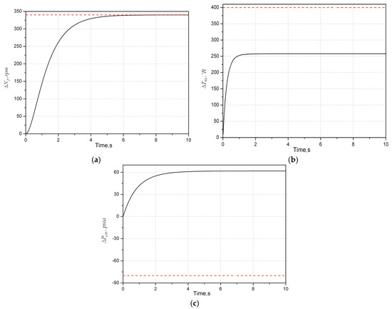
Figure 2.
Output response with optimal augmented monotonic tracking controller (OAMTC) limit regulator: positive set-point change. (a) Fan speed response; (b) high-pressure turbine outlet temperature response; and (c) high-pressure compressor outlet static pressure response.
In Figure 2, it is seen that the settling time is 3.5 s and output does not exceed its intended limit during the transient regime and settles at . As converges to its steady state value monotonically, moves away from its negative limit with no appearance of undershoot. In Figure 3, we can see that overlaps , which means that is active from until . Thus, the advantage of OAMTC is shown by the fact no switching is occurring in this min-max selector when it deals with transient violation problems. It should be noted that the larger the absolute values of poles to be placed at system and is, the better the OAMTC limit regulator works. One reason is that if the absolute values of the poles are enough large, the control rates may present a relationship like . By this way, some unnecessary switching can be avoided when the auxiliary outputs are far from their limits. Another reason is that once switching occurs, the corresponding output can track the target in fast speed without overshoot. This will be illustrated by the steady limit preservation example in the last part of the article. It is worth noting that the absolute values of the placed poles cannot be too large due to the limits of actuators in the real working conditions.
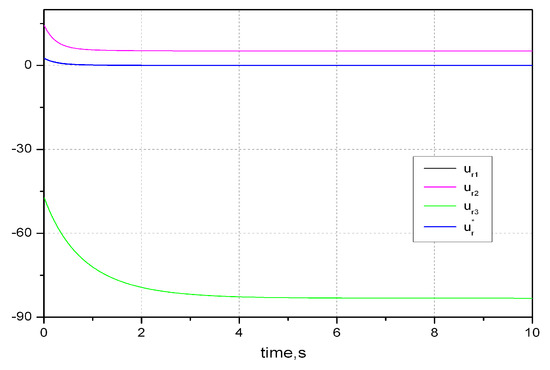
Figure 3.
Control rates with OAMTC limit regulator.
In order to show the robustness of OAMTC, some uncertainties are introduced to the plant parameters which may cause the tracking error to be nonzero. In real cases, uncertainties are mainly from the following two aspects: (1) characteristic variation in controlled plants, namely, the uncertainties caused by component aging, time varying parameters and outside disturbances; (2) uncertainties caused by modeling errors: the increasing complexity of the controlled plants with the development of technology means that the order of controlled plants increases, as well as the number of variables and the degree of nonlinearity. In the process of theoretical modeling, complex actual systems are often simplified into low order linear time invariant systems in order to be convenient for system analysis and controller design, which will introduce modeling errors inevitably. Now consider the following system where the uncertainties are introduced:
where denotes the uncertainty of plant parameters, in which are all real numbers and the random number is chosen within the range of .
Let , and . Applying the control law (12), for , yields sets of transient response curves as shown in Figure 4 and Figure 5. These figures show that when uncertainties exist in the plant parameters, the main output can always converge to the target reference with good performance while the auxiliary outputs can be kept within limits. It is also seen that though some uncertainties exist, which are composed of constant part, random number part and sine functions part, the transient responses of all outputs for different uncertainties remain monotonic. Note that if we only consider the constant part , which may transform the set of invariant zeros to a new fixed one. By contrast, the random number part and sine functions part may have a greater impact on the shape of output response because the invariant zeros are dynamic.
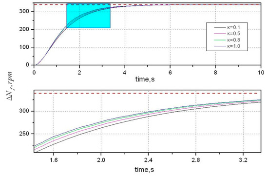
Figure 4.
Fan speed response with uncertainty in system parameters.
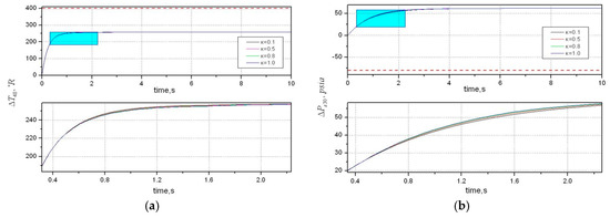
Figure 5.
Limited output response with uncertainty in system parameters. (a) High-pressure turbine outlet temperature response; and (b) high-pressure compressor outlet static pressure response.
Thus, we take different proportions of these part by changing the parameter and , respectively. It can be illustrated by two cases: (1) Case 1: Consider sine function part, let , and , and specify four different constants for parameter ; (2) Case 2: Consider random number part, let and , and also specify four different constants for parameter . The sets of output response curves are depicted in Figure 6, Figure 7 and Figure 8.
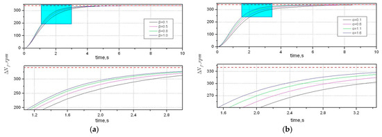
Figure 6.
Fan speed response with uncertainty in system parameters. (a) Case 1 by taking ; and (b) case 2 by taking .
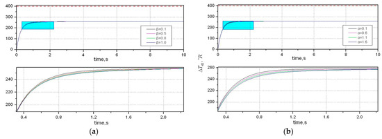
Figure 7.
High-pressure turbine outlet temperature response with uncertainty in system parameters. (a) Case 1; and (b) case 2.
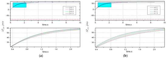
Figure 8.
High-pressure compressor outlet static pressure response with uncertainty in system parameters. (a) Case 1; and (b) case 2.
It can be seen that the main outputs can always converge to the target reference with no steady state errors and the auxiliary outputs can be kept within prescribed constraints. Note that whichever case we consider, the fan speed response still keeps monotonic in Figure 6 under different uncertainties, as well as the high-pressure turbine outlet temperature response in Figure 7 and the high-pressure compressor outlet static pressure response in Figure 8. In general, although the existence of uncertainties may leads to the loss of monotonicity, OAMTC still suppresses the occurrence of overshoot and undershoot and keeps the auxiliary outputs within limits effectively in transient regime.
Figure 2b shows that when tracks , will converge to 257.84. In order to show that the steady limit preservation is achieved, now we reduce the limit value of to 200°R. Assume that the tracking target is . The steady states for is . The simulation results are shown in Figure 9 and Figure 10. In Figure 10, we can see that is active from until , which causes to be regulated toward its limit. A regulator switching occurs near and becomes active for all subsequent time. Note that tracks the corresponding limit in fast speed without overshoot in Figure 9b, meanwhile, the responses in Figure 9a,c are all monotonic without overshoot. Thus, steady limit preservation is well achieved.
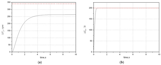
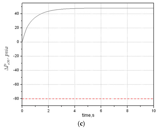
Figure 9.
Output response with OAMTC limit regulator: positive set-point change. (a) Fan speed response; (b) high-pressure turbine outlet temperature response; and (c) high-pressure compressor outlet static pressure response.
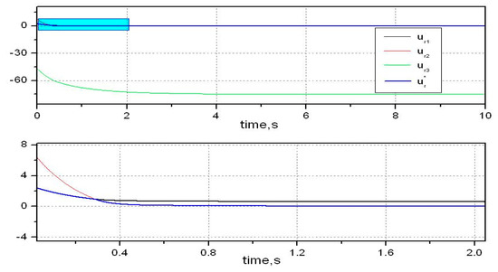
Figure 10.
Control rates with OAMTC limit regulator.
4. Conclusions
In this paper, an optimal angmented monotonic tracking controllers for an aircraft turbofan engine has been developed. In order to achieve monotonic tracking with zero steady-state error and guarantee transient limit protection of the auxiliary outputs, the eigenvalue and eigenvector placement method and genetic algorithms are employed to obtain an optimal solution. The key idea of this method is that the transient response of outputs is shaped in advance to eliminate overshoots, which may cause transient violations. After the OAMTC design process, the designed controllers are used to construct a min-max selector for testing the effectiveness. The simulation confirms the following two points: (1) an OAMTC controller presents strong robustness in two aspects: no steady state errors and the suppression of overshoot and undershoot in uncertainty-existing circumstances; (2) the min-max selector constructed by OAMTC controllers can avoid steady violation and transient violation effectively. Therefore, the control objectives can be well achieved by the described controller.
Acknowledgments
We are grateful for the financial support of the National Nature Science Foundation of China (No. 51276087).
Author Contributions
Jiakun Qin and Jinquan Huang contributed in developing the ideas of this research. Jiakun Qin and Muxuan Pan performed this research. All of the authors were involved in preparing this manuscript.
Conflicts of Interest
The authors declare no conflict of interest.
References
- Richter, H. A multi-regulator sliding mode control strategy for output-constrained systems. Automatica 2011, 47, 2251–2259. [Google Scholar] [CrossRef]
- May, R.D.; Garg, S. Reducing conservatism in aircraft engine response using conditionally active min-max limit regulators. In Proceedings of the ASME Turbo Expo: Turbine Technical Conference and Exposition, Copenhagen, Denmark, 11–15 June 2012.
- Thompson, A.; Hacker, J.; Cao, C. Adaptive Engine Control in the Presence of Output Limits. In Proceedings of the 2010 AIAA Infotech@Aerospace, Atlanta, GA, USA, 20–22 April 2010.
- Richter, H.; Litt, J.S. A novel controller for gas turbine engines with aggressive limit management. In Proceedings of the 47th AIAA/ASME/SAE/ASEE Joint Propulsion Conference & Exhibit, San Diego, CA, USA, 31 July–3 August 2011.
- Richter, H. Advanced Control of Turbofan Engines; Springer: New York, NY, USA, 2012; pp. 140–228. [Google Scholar]
- Richter, H. Multiple sliding modes with override logic: Limit management in aircraft engine controls. J. Guid. Control Dyn. 2012, 35, 1132–1142. [Google Scholar] [CrossRef]
- Richter, H. Control design with output constraints: Multi-regular sliding mode approach with override logic. In Proceedings of the 2012 American Control Conference (ACC), Montreal, QC, Canada, 27–29 June 2012.
- Schmid, R.; Ntogramatzidis, L. A unified method for the design of non-overshooting linear multivariable state-feedback tracking controllers. Automatica 2010, 46, 312–321. [Google Scholar] [CrossRef]
- Moore, B.C. On the flexibility offered by state feedback in multivariable systems beyond closed loop eigenvalue assignment. IEEE Trans. Autom. Control 1976, 21, 689–692. [Google Scholar] [CrossRef]
- Schmid, R.; Ntogramatzidis, L. The design of non-overshooting and non-undershooting multivariable state feedback tracking controllers. Syst. Control Lett. 2012, 61, 714–722. [Google Scholar] [CrossRef]
- Ntogramatzidis, L.; Trégouët, J.F.; Schmid, R.; Ferrante, A. A structural solution to the monotonic tracking control problem. 2014; arXiv:1412.1868. [Google Scholar]
- Garone, E.; Ntogramatzidis, L. Linear matrix inequalities for globally monotonic tracking control. Automatica 2015, 61, 173–177. [Google Scholar] [CrossRef]
- Richter, H. Advanced Control of Turbofan Engines; Springer: New York, NY, USA, 2012; pp. 20–28. [Google Scholar]
- Frederick, D.K.; Decastro, J.A.; Litt, J.S. User’s Guide for the Commercial Modular Aero-Propulsion System Simulation (C-MAPSS); NASA/ARL: Cleveland, OH, USA, 2007. [Google Scholar]
- Laguerre, E. On the Theory of Numeric Equations. 1883. Available online: http://sepwww.stanford.edu/oldsep/stew/laguerre.pdf (accessed on 14 November 2016).
- Jaw, L.C.; Mattingly, J.D. Engine modeling and simulation. In Aircraft Engine Controls: Design, System Analysis, and Health Monitoring; Schetz, J.A., Ed.; American Institute of Aeronautics & Astronautics (AIAA): Reston, VA, USA, 2009; pp. 37–66. [Google Scholar]
- Holland, J.H. Adaptation in Natural and Artificial Systems; The University of Michigan Press: Ann Arbor, MI, USA, 1975. [Google Scholar]
- Schaffer, J.D.; Caruana, R.A.; Eshelman, L.J.; Das, R. A study of control parameters affecting online performance of genetic algorithms for function optimization. In Proceedings of the Third International Conference on Genetic Algorithms, Fairfax, VA, USA, 4–7 June 1989; pp. 51–60.
- Xi, Y.G.; Chai, T.Y.; Yun, W.M. A review of genetic algorithm. Control Theory Appl. 1996, 6, 697–708. [Google Scholar]
© 2017 by the authors; licensee MDPI, Basel, Switzerland. This article is an open access article distributed under the terms and conditions of the Creative Commons Attribution (CC-BY) license (http://creativecommons.org/licenses/by/4.0/).