Abstract
In modern distributed energy systems (DES), focus is shifting from the conventional centralized approach towards distributed architectures. However, modeling and analysis of these systems is more complex, as it involves the interface of multiple energy sources with many different type of loads through power electronics converters. The integration of power electronics converters allows distributed renewable energy sources to become part of modern electronics power distribution systems (EPDS). It will also facilitate the ongoing research towards DC-based DES which is mostly composed of commercial DC-DC converters whose internal structure and parameters are unknown. For the system level analysis, the behavioral modeling technique is the only choice. Since most power electronics converters are non-linear systems and linear models can’t model their dynamics to a desired level of accuracy, hence non-linear modeling is required for accurate modeling. The non-linear modeling approach presented here aims to develop behavioral models that can predict the response of the system over the entire operating range. In this work, either a lookup table or a polytopic structure-based modeling technique is used. The technique is further applied to cascade and parallel connected converters, being two DES scenarios. First the procedure is verified via application to switching models in a simulation and then validated for commercial converters via experiments. The results show that the developed behavioral models accurately predict both the transient and steady state response.
1. Introduction
Modern distributed energy systems (DES) are comprised of multiple converters in which the loads are supplied by several low power converters, distributed throughout the system [1,2,3]. These systems include more than one source of energy, energy storage elements and several active and passive loads, either DC, AC or both. This implies the use of power electronics converters, required for power distribution over the entire system, hence also called electronic power distribution systems (EPDS). Today’s AC distribution systems are swiftly being replaced by DC distribution systems in many areas, motivated by the extensive use of electronic loads and integration of renewable energy sources into existing systems [3].
In the literature, DC-based energy distribution systems have been discussed for more electric aircraft (MEA) [4], electric/hybrid electric vehicles (HEVs) [5,6], all electric ships (AESs) [7], telecom applications [8,9] and for commercial and residential services [10,11]. The active nature of power electronics converters results in complex dynamic behavior during interconnection [12]. It makes the system level analysis of interconnected converters much more complicated, hence simulation tools are required to analyze and predict the behavior of complete systems [13,14]. Modeling and simulation are essential steps during the design stage of the complete system. The requirement to model power converters for system level analysis was first discussed in [15], and subsequently work has been done in this direction [2,16]. However conventional modeling techniques rely on the availability of information about the internal structure, i.e., topology, control, etc., of power electronics converters.
Modeling of power converters can be broadly categorized into white-box [2,17,18] and black-box approaches [19,20,21]. When all the necessary data to model the system’s behavior is available, then in such cases a white-box modeling approach is useful, while black-box or behavioral modeling refer to the modeling technique in which models for power converters and passive modules e.g., electromagnetic induction (EMI) filters are built without any available information about their internal design and components. The models of power electronics converters with minimum or no detail about the system are used to analyze the input-output behavior of the system. Such models can be easily interconnected with each other in various configurations, such as cascade, parallel, series and stacking form to build distributed energy systems.
The two port network-based linear behavioral modeling approach doesn’t require any details about the internal design and structure of the converter to be known. Linear behavioral modeling is well suited for converters whose behavior is linear over the entire operating range, e.g., un-regulated buck converters, but when applied to non-linear converters, it fails to give accurate results for large signal perturbations (load current or input voltage step). In fact it causes the operating point to move away from the region at which the converter was linearized, so non-linear behavioral modeling must be employed for power converters with strong non-linearities.
One type of non-linear behavioral modeling is based upon the series connection of a linear model with a non-linear function. If the non-linear function precedes the linear model, it is called a Hammerstein model and it is called a Wiener model when vice-versa. In [22] a hybrid Wiener-Hammerstein structure was developed using the data provided in the datasheets along with the transient response of the converter. It is based on the cascade combination of a non-linear static network and a linear dynamic network which cover the steady state and transient behavior of the converter, respectively. The non-linear hybrid terminal behavioral model proposed in [23], is based upon a Hammerstein approach, but it is limited to the converters that feature only static non-linearity and are dynamically linear. This approach models the static behavior, but is unable to accurately predict the dynamic behavior.
In this paper a look up table or polytopic structure-based non-linear behavioral modeling approach is applied to power converters exhibiting non-linear behavior. It is investigated first if each of the four g-parameters behave in a linear or non-linear way, as determined from the transient as well as the frequency response data. For the non-linear case, if the lookup table-based approach can’t handle the non-linearity, then the more complex polytopic structure-based approach is used. When a polytopic structure is used to model each dynamic system, it results in a highly accurate model, but at the cost of increased complexity and computational time, so there a trade-off must be made between accuracy and simplicity.
In modern distributed energy systems power electronics converters are often connected in various configurations, i.e., cascade, series, parallel and stacking. The non-linear behavioral modeling is further extended to analyze cascade and parallel configurations for system level analysis. First the behavioral models are built for individual converters and then the models are interconnected for the dynamic analysis of the complete system.
The behavioral modeling approach is first verified via simulation using the MATLAB/Simulink Software package (MathWorks, Natick, MA, USA) [24]. Then the approach is validated experimentally for commercial DC-DC converters. Both in the case of verification via simulation and validation via experiment, the results from the actual converters are compared with the behavioral models. The close agreement of the results demonstrates that the non-linear behavioral modeling approach is able to predict the transient as well as the steady responses of the modeled systems with high accuracy.
The paper is organized as follows: Section 2 explains the two port network-based behavioral modeling of DC-DC converters. Section 3 covers the non-linear behavioral modeling. Section 4 explains the modeling of a distributed energy system. Finally Section 5 gives the conclusion of the work presented.
2. Behavioral Modeling of DC-DC Converters
The two port network-based modeling technique was first applied to DC-DC converters in [15,25], while the first identification procedure was proposed in [21]. It is based upon the measurement of frequency responses via small signal perturbations, obtained using a network analyzer. Another method, which doesn’t require expensive equipment is based upon the step change in transient response, the time domain data is then used for the identification of frequency responses [26].
The g-parameters-based two port network is a hardware-oriented behavioral modeling approach, which doesn’t require any knowledge about the internal design of the converter. Hence there is no difference in the modeling methodology for various type of converters, i.e., buck, boost etc. The complete model is based upon the measurement and identification of four linear time invariant (LTI) models as transfer functions in the Laplace domain, i.e., output impedance , back current gain , audiosusceptibility and input admittance . The two-port network shown in Figure 1 represents un-terminated model, so the dynamic system based upon it should model only the internal dynamics of the converter. To achieve this the measurement setup should have almost no interaction either with the source or load. This is possible if the converter is fed from a low output impedance voltage source and connected to an electronic load in constant current sink mode [27]. Using such a decoupling procedure the influence of external elements such as filters and other converters can be removed from the measurements.
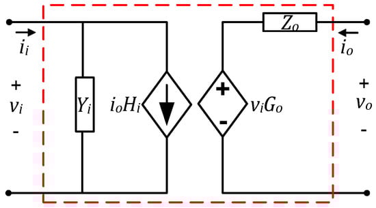
Figure 1.
G-parameters based two port network model for DC-DC converter.
The g-parameter set required to be measured is given in Equation (1):
The input variables of the two port network are the input voltage and output current while the output variables are the output voltage and input current .
The problem with linear two port network-based modeling is that it is assumed that converters are mildly non-linear [1]. For linear or mildly non-linear dynamic relations a single LTI model is sufficient. In practice most of the power electronic converters are non-linear systems, so some non-linear behavioral modeling technique must be employed. The non-linear behavioral modeling technique employed here differs from the linear behavioral modeling shown in Figure 1 in the sense that single LTI models are replaced by a lookup table or a polytopic structure.
The modification of the linear behavioral model requires some sort of iteration of the linearization process applied at different operating points. In the end all these linear models can be unified into a single non-linear structure called polytopic modeling. A polytopic structure is built by the combination of several local LTI models. In it, small perturbations are applied on the input variables at different operating points. The use of a number of local linear models for a non-linear system have been used in several other applications, e.g., the fuzzy logic-based systems called Takagi-Sugeno models [28,29], neural network-based systems [30,31], mechanics [32,33], robotics [34], aeronautics [35] and electromechanical systems [36]. The application of polytopic modeling to power electronic systems is discussed in [37,38].
In case of polytopic structure-based non-linear behavioral modeling, the system is modeled by a set of linear models which are valid for different operating points. These local linear models are then combined by interpolation to cover the entire operating range. When the operating point changes, the model makes a smooth transition from one local linear model to another. The width of the space for each local model is chosen such as the system’s behavior is linear within a sub-space. Linear models are measured and identified for each sub-space. Then with the change in operating condition, the shift from one operating point to another is made by using some validity function.
For a general non-linear system:
where , and represent the state, input and output variables respectively. The mathematical representation of the polytopic structure is:
is called validity or interpolation function, describing the region where the local models are valid, and it may be a function of either or . To avoid switching and have a smooth transition from one local model to another, the validity function should satisfy the condition, i.e.,:
Furthermore it is also necessary that the sum of weighting functions at any point within the entire operating space should be equal to one:
The weighting functions are placed in the center of each sub-space, such that:
A few of the commonly used weighting functions are triangular [28], sigmoid, double sigmoid and trapezoidal functions. The triangular function used in this work is defined by Equation (7):
where the parameters and represent the end points of the triangle and shows the center.
The partitioning of the operating region into sub-spaces mainly depends upon the non-linearity shown by the converter over the entire range [39]. The center of the sub-space is the point at which the frequency response function is measured. If the number of local linear models obtained are unable to predict the response accurately over a certain region, then more local models should be obtained by further reducing the width of the sub-space.
The output of local linear models with input and weighting function can be calculated by weighting the validity function values and adding them together:
When the local linear models are dependent on two variables, then 2-d polytopic modeling is employed in which several 1-d polytopic models are grouped together, but increase in the number of variables for polytopic modeling cause an exponential increase in the number of local models.
In order to identify the dynamic models from the measured data, parametric and non-parametric methods can be used [40]. Parametric methods are applied to data obtained either from frequency or transient response measurements, from which transfer functions or state-space models are obtained. Among the available model structures, a few commonly used ones are: ARX, ARMAX, OE, BJ and the state-space model, and the most appropriate one should be selected [40,41,42]. A proper model structure is important for accurate identification. Also, the order of the model plays its role in terms of fitting accuracy. Normally there is a trade-off between accuracy and simplicity of the model. Once the transfer functions are identified, behavioral model is constructed and implemented in MATLAB/Simulink.
3. Non-Linear Behavioral Modeling
3.1. Verification via Simulation
The aim of this section is to explain the non-linear behavioral modeling procedure and verify it by simulation. A switch model of a regulated DC-DC buck converter (30/10 V, 100 W) is simulated using MATLAB/Simulink. The dynamic systems as transfer functions are subsequently identified from step transient response data. Depending upon the behavior exhibited by a dynamic relation, either a linear or a non-linear model is used. Finally the response of the behavioral and switching model is compared.
The step change in the output current is applied to identify output impedance and back current gain. Also step changes in the input voltage are used to identify input admittance and audiosusceptibility. The step tests are performed such that only one input signal is perturbed at a time, while the other is kept constant. The step transient response data is used for the identification of corresponding frequency responses, where the midpoint of the step change is considered as the operating point. The transient as well as corresponding frequency responses are given for each case.
To evaluate output impedance, the output voltage response is analyzed for step changes in the load current. In first case the input voltage is kept constant and a load current step with different values is applied as shown in Figure 2a,b. In the second case the input voltage is changed for the same load current step shown in Figure 2c,d. It can be seen that if the input voltage is kept constant for each load step, the response is same, thus a single LTI model is sufficient. However in the second case when the same load step is applied at different input voltage values, both the transient as well as the frequency response vary, indicating non-linearity.
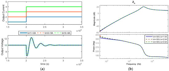
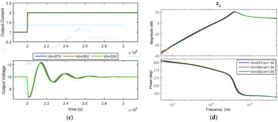
Figure 2.
Transient and frequency responses as a function of (a,b) load current; and (c,d) input voltage.
Figure 3 shows a 1-d polytopic model for output impedance, where the local linear models are evaluated for different values of input voltage.
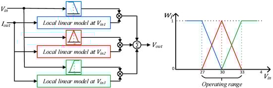
Figure 3.
1-d polytopic model.
To evaluate back current gain, the input current response is analyzed for step change in load current. In first case the input voltage is kept constant and load current step is applied at different values as shown in Figure 4a,b. In the second case the input voltage is changed for the same load current step shown in Figure 4c,d. It can be seen that in either case, both transient as well as the frequency response vary, indicating 2-d non-linearity. It should be noted that for step change from 2–3 A and 3–4 A the input current values also increases, but the increase is subtracted to match the current value at 1 A, so that comparison for all the responses can be made easily. A similar approach is also used in the figures ahead where there is an increase in input current.
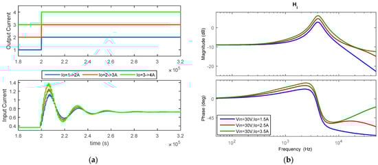
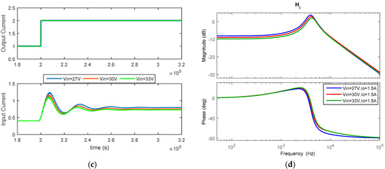
Figure 4.
Transient and frequency responses as a function of (a,b) load current; and (c,d) input voltage.
Figure 5 shows a 2-d polytopic model for back current gain, where first the local linear models are evaluated for different values of input voltage , and then for each value of models are evaluated for different values of .
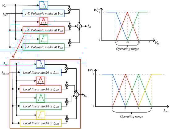
Figure 5.
2-d polytopic model.
To evaluate the audiosusceptibility, the output voltage response is analyzed for step changes in input voltage. In the first case the load current is kept constant and different values of the input voltage step are applied as shown in Figure 6a,b. In the second case the load current is changed for the same input voltage step as shown in Figure 6c,d.
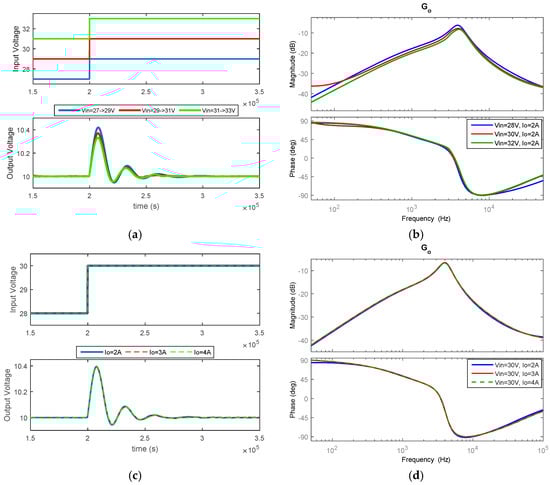
Figure 6.
Transient and frequency responses as a function of (a,b) input voltage; and (c,d) load current.
It can be seen that if the load current is kept constant for each voltage step, both transients as well as frequency responses vary with a constant gain, so a lookup table-based approach is used, where the input voltage serves as an input that looks for a constant multiplier to be multiplied with the LTI model, i.e., a transfer function measured at the nominal operating point. However in the second case when the same voltage step is applied at different values of load current, the response is the same. Hence a single LTI model is sufficient.
Figure 7 shows the representation of 1-d lookup table structure.
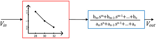
Figure 7.
1-d lookup table model.
To evaluate the input admittance, the input current response is analyzed for step changes in input voltage. In the first case the load current is kept constant and different value input voltage steps are applied as shown in Figure 8a,b. In the second case the load current is changed for the same input voltage step as shown in Figure 8c,d.
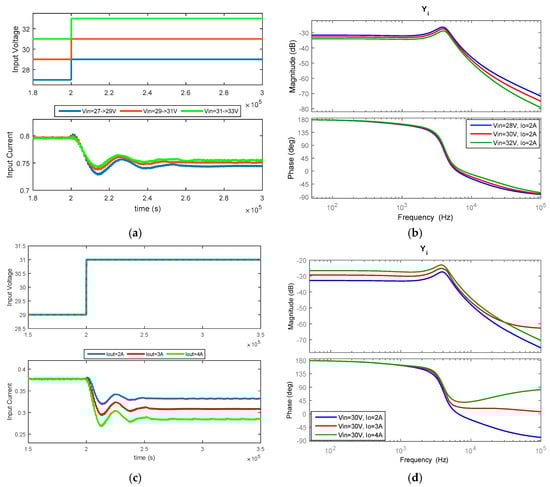
Figure 8.
Transient and frequency responses as a function (a,b) input voltage; and (c,d) load current.
It can be seen that in both cases the responses are related by a linear gain, so a 2-d lookup table is used to model this non-linear dynamic relation.
Figure 9 shows the 2-d lookup table structure.
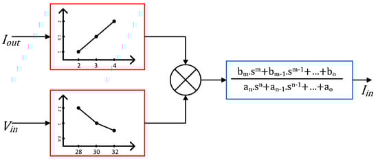
Figure 9.
2-d lookup table model.
To verify the modeling done for four g-parameters a step change in load current is applied. The model is verified with data that is different from that used to build the model [40]. The response of the switch model for each of the output variables is compared against the behavioral model and their close match suggests the effectiveness of the model, as shown in Figure 10. It is thus verified that the developed behavioral model has the capability to accurately represent the dynamic behavior of the converter over a wide operating region.
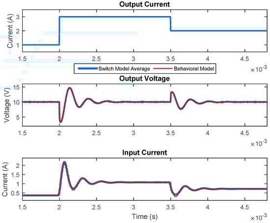
Figure 10.
Non-linear behavioral model verification.
For further verification of the model, root mean square deviation (RMSD) values are calculated for the above waveforms. The switch model’s response is compared with the behavioral model’s response for output voltage and input current:
3.2. Validation via Experiment
In this section the non-linear behavioral modeling procedure developed in the previous section is experimentally validated for a commercial DC-DC converter, i.e., a SD-100B-12 (30/12 V, 100 W) [43]. Figure 11 shows the identified frequency responses for , and , while in case of the output voltage remains unperturbed to change in input voltage or load current so its value is introduced as a constant in the model.
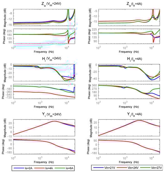
Figure 11.
Frequency responses for , and of commercial converter.
In order to validate the performance of the behavioral model, step changes in the load current are applied. The input and output signals are recorded using an oscilloscope and then imported into MATLAB. The actual load current from the experiment is applied to the behavioral model and its output is compared with that of the experiment. In Figure 12 it can be clearly seen that the response of the behavioral model closely matches that of the actual converter.
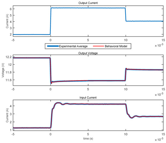
Figure 12.
Experimental validation for non-linear behavioral modeling.
The RMSD values are also calculated for the experimentally obtained output voltage and input current and compared with its corresponding behavioral model’s response:
The results show that the non-linear behavioral model is able to predict not only the steady state value, but also the transient response, i.e., overshoot and natural frequency of oscillations both in the case of simulation and experiment.
4. Modeling of Distributed Energy Systems
Behavioral models based upon two port networks are suitable for the system level design and analysis of larger distributed energy systems. The two terminal nature of these models makes it an appropriate choice for cascade and parallel connected converters. Such configurations are commonly found in modern EPDS [8,9], so it is necessary to build models for the analysis of such interconnected systems.
The transient dynamics of the interconnected converters are not only dependent upon the converters themselves, but also on the elements to which they are connected [44,45], so it is investigated whether the models developed for converters working in standalone mode remain valid when they become part of a distributed system. Here two commonly used configurations, i.e., cascade and parallel, are analyzed.
4.1. Parallel Connected Converters
The advantage of converters connected in parallel configuration allows for online replacement of any converter which stops working, thus the system keeps running uninterruptedly. The parallel operation of DC-DC converters may also be employed for loads which demand high current. It is also often used in distributed systems to improve the reliability of N+1 power converters and also reduce stress on each converter. Figure 13 shows two parallel connected converters, represented in terms of their g-parameters.
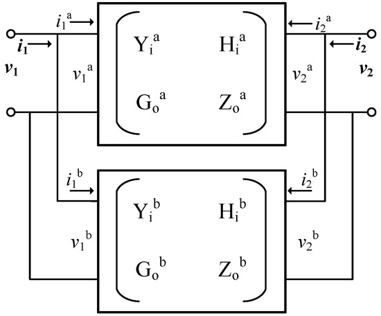
Figure 13.
Parallel connected converters as two port network.
First the frequency responses of each converter are measured individually. The matrix representation of both is given below:
When the two systems are connected in parallel, they can be represented as a single system:
As per the procedure discussed in [46], the g-parameters of the overall system are:
4.1.1. Model Verification via Simulation
For verification via simulation two un-regulated buck converters are connected in parallel. First the two converters are individually operated at the following same operating point:
Figure 14 shows the g-parameters measured for each converter and for the parallel system. Since both the converters have identical parameters and have the same operating point, they have similar frequency responses, as shown by the “blue” and “green” colored plots.
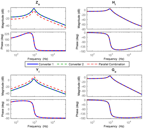
Figure 14.
Frequency responses for individual and parallel connected converters.
To verify the behavioral model of the overall parallel system, step change in load current is applied at the input and Figure 15 shows the output voltage and input current response comparison for the switch and behavioral model.
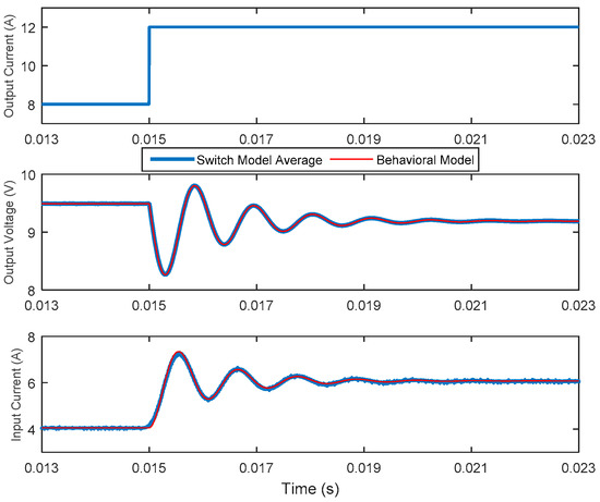
Figure 15.
Parallel configuration’s modeling verification.
4.1.2. Model Validation via Experiment
The experimental setup is based upon two commercial DC-DC converters, i.e., an SD-100B-12 (30/12V, 100W, MEAN WELL, New Taipei City, Taiwan) and an SD-200B-12 (30/12V 200W), connected to an electronic load. The passive current sharing method is employed and a diode is used with each converter for output decoupling. Due to the passive current sharing, the current drawn from each converter depends upon the output impedance of the two. Hence each converter must be modeled separately.
Using the same procedure as employed in the simulation, first the two converters are individually operated at certain operating point. The g-parameters are measured for each converter and then Equation (14) is used to obtain the equivalent frequency response for the parallel system, which is then used to construct the behavioral model of the parallel connected converters:
To validate the behavioral model of the parallel system, a step change in load current is applied and the actual input as well as the output signals from the experiment are recorded. The experimental step load current signal is applied to the behavioral model setup constructed in MATLAB and the actual output from experiment is compared with the output of behavioral model, shown in Figure 16.
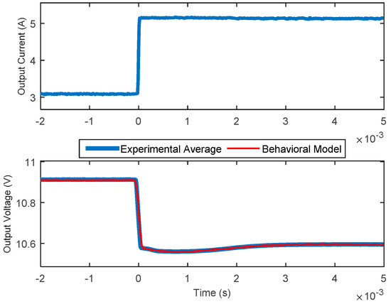
Figure 16.
Parallel configuration’s modeling validation.
Both in the case of simulation as well as the experiments the results match pretty well, suggesting that the behavioral model developed for converters obtained in standalone mode remains valid when they are connected in parallel configuration.
4.2. Cascade Connected Converters
Figure 17 shows two cascade connected converters, represented in terms of their g-parameters.
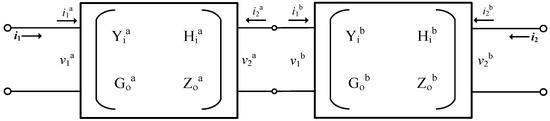
Figure 17.
Cascade connected converters as two port network.
First the frequency responses of each converter are measured individually. The matrix representation of both is given below:
When the two systems are connected in cascade, they can be represented as a single system:
The equivalent g-parameters of cascade connected converters are represented as [46]:
4.2.1. Model Verification via Simulation
For verification via simulation a regulated boost converter and an un-regulated buck converter are connected in cascade. First the two converters are individually operated at the following operating points:
Figure 18 shows the g-parameters measured for each converter and for cascade system.
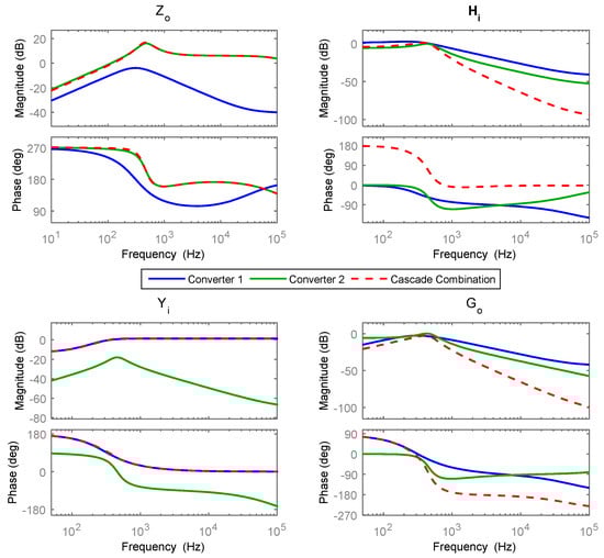
Figure 18.
Frequency responses for individual and cascade connected converters.
To verify the behavioral model of the overall cascade system, a step change in load current is applied and responses for output voltage and input current are compared. Figure 19 shows the equivalent behavioral model where the transfer functions used are computed using Equation (20).
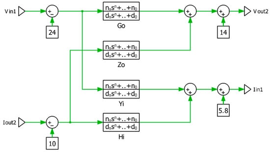
Figure 19.
Model for cascade connected converters.
However, when the behavioral model’s response is compared with the actual switch model response, there is slight mismatch between the results. After some further research it is found that the dynamic response to a step change in load current of an un-regulated buck converter is different when it becomes part of a cascade network compared to standalone mode of operation. Figure 20 shows the step load change response of the un-regulated buck converter in isolated vs. cascade mode.
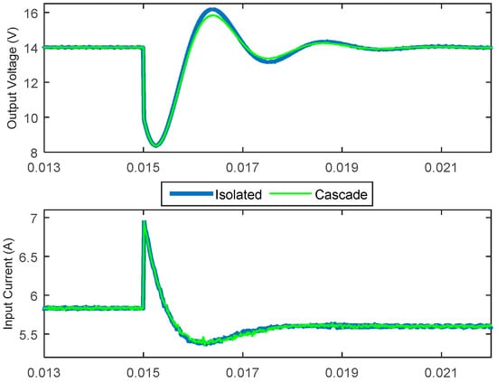
Figure 20.
Step load change response for isolated vs. cascade mode.
Therefore, in order to include the effect of these small dynamic changes the frequency responses are measured while the two converters are connected in cascade configuration. Then a modified behavioral model is built as shown in Figure 21, based upon each converter’s frequency responses.
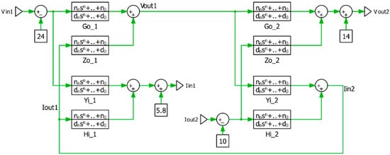
Figure 21.
Modified model for cascade connected converters.
Now the result of step change in load current for the switch model is compared with the response of original and modified behavioral model. Figure 22 shows that there is slight mismatch for the switch and original model, while the modified model results are in good agreement with the actual switch model results.
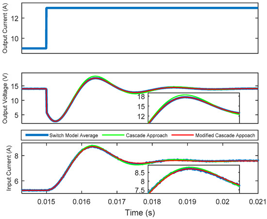
Figure 22.
Cascade configuration’s modeling verification.
4.2.2. Model Validation via Experiment
The experimental setup is based upon two commercial DC-DC converters, i.e., an SD-100B-24 (30/24 V, 100 W) and an SD-100B-12 (24/12 V 100 W), connected to an electronic load.
A modified behavioral modeling approach is used for experimental validation as well. The g-parameters are measured for each converter, while connected in cascade mode and then Equation (20) is used to obtain the equivalent frequency response for the overall cascade system, which is then used to construct the behavioral model of the cascade connected converters. The measurements are done at the following operating points:
To validate the behavioral model of the cascade system, step changes are applied in the load current and the actual input as well as the output signals from the experiment are recorded. The experimental step load current signal is applied to the behavioral model constructed in MATLAB and the output signals from experiment are compared with that of the behavioral model, shown in Figure 23.
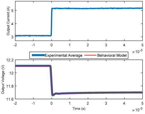
Figure 23.
Cascade configuration’s modeling validation.
The results from the actual experiment match with those of the behavioral model, validating the procedure described for the analysis of overall cascade and parallel connected converters.
5. Conclusions
The integration of several different energy sources thorough power electronics converters to become electronic power distribution system also requires simulation tools for the design and analysis of such systems. As most of the power converters are provided by different vendors, this means less data is available for their modeling. The two-port network-based behavioral modeling approach provides the solution as it relies upon experimental data to model the input-output behavior of the system. It also enables interconnection of different types of power electronics devices for system level analysis from the design perspective. The switching action of power electronics devices causes them to behave in a non-linear way and linear modeling techniques fail to model the entire operating range accurately. A non-linear modeling methodology is presented based upon either a lookup table or a polytopic structure for different dynamic relations. The concept is further extended and applied to two types of distributed energy system, i.e., cascade and parallel configuration. All the work done is first verified by simulation in MATLAB/Simulink and then validated experimentally for commercial converters. Both in the cases of simulation and experiments, the results from the actual system match well with the developed behavioral model, thus proving the effectiveness of the presented work.
Author Contributions
Xiancheng Zheng and Husan Ali contributed equally to the research described in this work. Xiancheng Zheng and Husan Ali conceived and designed the experiments. Husan Ali performed the experiments, analyzed the data and wrote the paper. Xiaohua Wu and Haider Zaman provided significant comments and technical feedback throughout the research. Xiaohua Wu and Shahbaz Khan reviewed and improved the paper.
Conflicts of Interest
The authors declare no conflict of interest.
References
- Boroyevich, D.; Burgos, R.; Arnedo, L.; Wang, F. Synthesis and integration of future electronic power distribution systems. In Proceedings of the Power Conversion Conference (PCC’07), Nagoya, Japan, 2–5 April 2007.
- Franz, G.A.; Ludwig, G.W.; Steigerwald, R.L. Modelling and simulation of distributed power systems. In Proceedings of 21st Annual IEEE Power Electronics Specialists Conference (PESC’90), San Antonio, TX, USA, 11–14 June 1990.
- Dragicevic, T.; Vasquez, J.C.; Guerrero, J.M.; Skrlec, D. Advanced LVDC electrical power architectures and microgrids: A step toward a new generation of power distribution networks. IEEE Electr. Mag. 2014, 2, 54–65. [Google Scholar] [CrossRef]
- Izquierdo, D.; Azcona, R.; Cerro, F.J.L.; Fernandez, C.; Delicado, B. Electrical power distribution system (HV270DC), for application in more electric aircraft. In Proceedings of the 25th Annual IEEE Applied Power Electronics Conference and Exposition (APEC), Palm Springs, CA, USA, 21–25 February 2010.
- Jayabalan, R.; Fahimi, B.; Koenig, A.; Pekarek, S. Applications of power electronics-based systems in vehicular technology: State-of-the art and future trends. In Proceedings of the 35th Annual IEEE Power Electronics Specialists Conference (PESC 04), Aachen, Germany, 20–25 June 2004.
- Emadi, A.; Lee, Y.J.; Rajashekara, K. Power electronics and motor drives in electric, hybrid electric, and plug-in hybrid electric vehicles. IEEE Trans. Ind. Electron. 2008, 55, 2237–2245. [Google Scholar] [CrossRef]
- Ciezki, J.G.; Ashton, R.W. Selection and stability issues associated with a navy shipboard DC zonal electric distribution system. IEEE Trans. Power Deliv. 2000, 15, 665–669. [Google Scholar] [CrossRef]
- Schulz, W. ETSI standards and guides for efficient powering of telecommunication and datacom. In Proceedings of the IEEE 29th International Telecommunications Energy Conference (INTELEC), Rome, Italy, 30 September–4 October 2007.
- Miftakhutdinov, R. Power distribution architecture for tele- and data communication system based on new generation intermediate bus converter. In Proceedings of the IEEE 30th International Telecommunications Energy Conference (INTELEC), San Diego, CA, USA, 14–18 September 2008.
- Salomonsson, D.; Sannino, A. Low-voltage DC distribution system for commercial power systems with sensitive electronic loads. IEEE Trans. Power Deliv. 2007, 22, 1620–1627. [Google Scholar] [CrossRef]
- Wu, T.-F.; Chen, Y.-K.; Yu, G.-R.; Chang, Y.-C. Design and development of DC-distributed system with grid connection for residential applications. In Proceedings of the IEEE 8th International Conference on Power Electronics and ECCE Asia (ICPE&ECCE), Jeju, Korea, 30 May–3 June 2011.
- Sanz, M.; Valdivia, V.; Zumel, P.; Moral, D.L.; Fernández, C.; Lázaro, A.; Barrado, A. Analysis of the Stability of Power Electronics Systems: A Practical Approach. In Proceedings of the 29th Annual IEEE Applied Power Electronics Conference and Exposition (APEC), Charlotte, NC, USA, 16–20 March 2014.
- Feng, X.; Liu, J.; Lee, F.C. Impedance specifications for stable DC distributed power systems. IEEE Trans. Power Electron. 2000, 17, 157–162. [Google Scholar] [CrossRef]
- Liu, J.; Feng, X.; Lee, F.C.; Boroyevich, D. Stability margin monitoring for DC distributed power systems via perturbation approaches. IEEE Trans. Power Electron. 2003, 18, 1254–1261. [Google Scholar]
- Cho, B.H.; Lee, F.C.Y. Modeling and analysis of spacecraft power systems. IEEE Trans. Power Electron. 1988, 3, 44–54. [Google Scholar] [CrossRef]
- Karimi, K.J.; Booker, A.; Mong, A. Modeling, simulation, and verification of large DC power electronics systems. In Proceedings of the 27th Annual IEEE Power Electronics Specialists Conference (PESC’96), Baveno, Italy, 23–27 June 1996.
- Tam, K.-S.; Yang, L. Functional models for space power electronic circuits. IEEE Trans. Aerosp. Electron. Syst. 1995, 31, 288–296. [Google Scholar]
- Wang, R.; Liu, J.; Wang, H. Universal approach to modeling current mode controlled converters in distributed power systems for large-signal subsystem interactions investigation. In Proceedings of the 22nd Annual IEEE Applied Power Electronics Conference (APEC 2007), Anaheim, CA, USA, 25 February–1 March 2007.
- Prieto, R.; Laguna-Ruiz, L.; Oliver, J.A.; Cobos, J.A. Parameterization of DC/DC converter models for system level simulation. In Proceedings of the European Conference on Power Electronics and Applications, Aalborg, Denmark, 2–5 September 2007.
- Oliver, J.A.; Prieto, R.; Romero, V.; Cobos, J.A. Behavioral modeling of DC-DC converters for large-signal simulation of distributed power systems. In Proceedings of the 21st Annual IEEE Applied Power Electronics Conference and Exposition (APEC’06), Dallas, TX, USA, 19–23 March 2006.
- Arnedo, L.; Burgos, R.; Wang, F.; Boroyevich, D. Black-box terminal characterization modeling of DC-to-DC Converters. In Proceedings of the 22nd Annual IEEE Applied Power Electronics Conference (APEC 2007), Anaheim, CA, USA, 25 February–1 March 2007.
- Oliver, J.; Prieto, R.; Cobos, J.; Garcia, O.; Alou, P. Hybrid Wiener-Hammerstein structure for grey-box modeling of DC-DC converters. In Proceedings of the 24th Annual IEEE Applied Power Electronics Conference and Exposition (APEC), Washington, DC, USA, 15–19 February 2009.
- Cvetkovic, I.; Boroyevich, D.; Mattavelli, P.; Lee, F.C.; Dong, D. Nonlinear, hybrid terminal behavioral modeling of a dc-based nanogrid system. In Proceedings of the 26th Annual IEEE Applied Power Electronics Conference and Exposition (APEC), Orlando, FL, USA, 6–11 March 2011.
- MathWorks. Available online: http://www.mathworks.com (accessed on 5 April 2016).
- Maranesi, P.G.; Tavazzi, V.; Varoli, V. Two-port characterization of PWM voltage regulators at low frequencies. IEEE Trans. Ind. Electron. 1988, 35, 444–450. [Google Scholar] [CrossRef]
- Valdivia, V.; Barrado, A.; Lazaro, A.; Zumel, P.; Raga, C. Easy modeling and identification procedure for “black box” behavioral models of power electronics converters with reduced order based on transient response analysis. In Proceedings of the 24th Annual IEEE Applied Power Electronics Conference and Exposition (APEC), Washington, DC, USA, 15–19 February 2009.
- Arnedo, L.; Boroyevich, D.; Burgos, R.; Wang, F. Un-terminated frequency response measurements and model order reduction for black box terminal characterization models. In Proceedings of the 23rd Annual IEEE Applied Power Electronics Conference and Exposition (APEC), Austin, TX, USA, 24–28 February 2008.
- Takagi, T.; Sugeno, M. Fuzzy identification of systems and its applications to modeling and control. IEEE Trans. Syst. Man Cybern. 1985, 1, 116–132. [Google Scholar] [CrossRef]
- Zhang, H.; Liu, D. Fuzzy Modeling and Fuzzy Control, 1st ed.; Birkhäuser Basel: Boston, MA, USA, 2006. [Google Scholar]
- Murray-Smith, R.; Kenneth, H. Local model architectures for nonlinear modelling and control. In Neural Network Engineering in Dynamic Control Systems; Hunt, K.J., Irwin, G.R., Warwick, K., Eds.; Springer: London, UK, 1995; pp. 61–82. [Google Scholar]
- Lin, F.-J.; Huang, M.-S.; Hung, Y.-C.; Kuan, C.-H.; Wang, S.-L.; Lee, Y.-D. Takagi-sugeno-kang type probabilistic fuzzy neural network control for grid-connected LiFePO4 battery storage system. IET Power Electron. 2013, 6, 1029–1040. [Google Scholar] [CrossRef]
- Fujimori, A.; Ljung, L. A polytopic modeling of aircraft by using system identification. In Proceedings of the International Conference on Control and Automation, Budapest, Hungary, 27–29 June 2005.
- Grof, P.; Petres, Z.; Gyeviki, J. Polytopic model reconstruction of a pneumatic positioning system. In Proceedings of the 5th International Symposium on Applied Computational Intelligence and Informatics, Timisoara, Romania, 28–29 May 2009.
- Chen, J.; Li, R.; Cao, C. Convex polytopic modeling for flexible joints industrial robot using TP-model transformation. In Proceedings of the IEEE International Conference on Information and Automation (ICIA), Hailar, China, 28–30 July 2014.
- Huang, Y.; Sun, C.; Qian, C.; Zhang, J.; Wang, L. Polytopic LPV modeling and gain-scheduled switching control for a flexible air-breathing hypersonic vehicle. J. Syst. Eng. Electron. 2013, 24, 118–127. [Google Scholar] [CrossRef]
- Ren, L.; Irwin, G.W.; Flynn, D. Nonlinear identification and control of a turbo generator an on-line scheduled multiple model controller approach. IEEE Trans. Energy Convers. 2005, 20, 237–245. [Google Scholar] [CrossRef]
- Sudhoff, S.D.; Glover, S.F.; Zak, S.H.; Pekarek, S.D.; Zivi, E.J.; Delisle, D.E.; Clayton, D. Stability analysis methodologies for dc power distribution systems. In Proceedings of the 13th International Ship Control Systems Symposium (SCSS), Orlando, FL, USA, 7–9 April 2003.
- Arnedo, L.; Boroyevich, D.; Burgos, R.; Wang, F. Polytopic Black-Box modeling of DC-DC converters. In Proceedings of the 39th Annual IEEE Power Electronics Specialists Conference (PESC), Rhodes, Greece, 15–19 June 2008.
- Nelles, O. Axes-oblique partitioning strategies for local model networks. In Proceedings of the IEEE International Symposium on Intelligent Control, Munich, Germany, 4–6 October 2006.
- Ljung, L. System Identification—Theory for the User, 2nd ed.; Prentice Hall: Upper Saddle River, NJ, USA, 1999. [Google Scholar]
- Ljung, L. Integrated frequency-time domain tools for system identification. In Proceedings of the American Control Conference, Boston, MA, USA, 30 June–2 July 2004.
- Ljung, L.; Glad, T. Modeling of Dynamic Systems; Prentice Hall: Upper Saddle River, NJ, USA, 1994. [Google Scholar]
- MeanWell. Available online: http://www.meanwell.com/webapp/product/search.aspx?prod=SD-100 (accessed on 20 July 2016).
- Hankaniemi, M.; Suntio, T.; Sippola, M.; Oyj, E. Characterization of regulated converters to ensure stability and performance in distributed power supply systems. In Proceedings of the 27th International Telecommunications Conference (INTELEC), Berlin, Germany, 18–22 September 2005.
- Hankaniemi, M.; Karppanen, M.; Suntio, T. Load-imposed instability and performance degradation in a regulated converter. IEE Proc. Electr. Power Appl. 2006, 153, 781–786. [Google Scholar] [CrossRef]
- Guotian, Y. The g parameters of series, parallel, cascade connection in two-port networks. J. Xuzhou Norm. Univ. 1993, 11, 29–33. [Google Scholar]
© 2017 by the authors; licensee MDPI, Basel, Switzerland. This article is an open access article distributed under the terms and conditions of the Creative Commons Attribution (CC-BY) license (http://creativecommons.org/licenses/by/4.0/).