Article

Wind Profiles and Wave Spectra for Potential Wind Farms in South China Sea. Part II: Wave Spectrum Model

1
Division of Ocean Science and Technology, Graduate School at Shenzhen, Tsinghua University, Shenzhen 518055, China
2
School of Environment, Tsinghua University, Beijing 100084, China
*
Author to whom correspondence should be addressed.
Energies 2017, 10(1), 127; https://doi.org/10.3390/en10010127
Submission received: 1 October 2016 / Revised: 13 December 2016 / Accepted: 29 December 2016 / Published: 20 January 2017

Abstract

:
Along with the commercialization of offshore wind energy in China, the South China Sea has been identified as ideal for constructing offshore wind farms, especially for farms consisting of floating wind turbines over deep waters. Since the wind profiles and wave spectra are somewhat primitive for the design of an offshore wind turbine, engineering models describing the wind and wave characteristics in the South China Sea area are necessary for the offshore wind energy exploitation given the meteorological, hydrological, and geographical differences between the South China Sea and the North/Norwegian Sea, where the commonly used wind profile and wave spectrum models were designated. In the present study; a series of numerical simulations were conducted to reveal the wave characteristics in the South China Sea under both typhoon and non-typhoon conditions. By analyzing the simulation results; the applicability of the Joint North Sea Wave Project (JONSWAP) spectrum model; in terms of characterizing the wind-induced wave fields in the South China Sea; was discussed. In detail; the key parameters of the JONSWAP spectrum model; such as the Phillips constant; spectral width parameter; peak-enhancement factor, and high frequency tail decay; were investigated in the context of finding suitable values.

1. Introduction

Along with the development of renewable and sustainable energy exploitation technology, the ample wind energy available over the sea has attracted attention from scientists, engineers, and policymakers [1]. While the construction and maintenance of a wind farm at an inland site has already reached a mature stage, the techniques required for harvesting offshore wind energy are still a topic for academic research. To harvest wind energy over deep waters (>50 m), a floating foundation which could support an ordinary, commercialized wind turbine is an appealing choice [2,3]. In terms of exploiting offshore wind energy through floating wind farms, the South China Sea has been recognized as an ideal region [4]. Before the construction of floating wind farms, the designer should calculate the wind and wave loads acting on the floating foundations and on the turbine. This explicit demand in turn requires engineering models depicting the characteristics of winds and waves observed in the South China Sea area. To be more specific, a wind profile model and a wave spectrum model are hence necessary and should be of concern for both academic research and engineering practices.
Generally speaking, two situations should be taken into consideration when investigating either the wind profile model or the wave spectrum model, namely the normal situation corresponding to the Douglas sea scale [5] varying from the value 0 to 4 and the extreme situation corresponding to the Douglas sea scale exceeding the value 4. While the working performance of a certain offshore wind turbine is evaluated under the normal situation, the extreme situation is used to do the safety check to ensure the survivability of the foundation and the turbine.
Two wind profile models, corresponding to the normal and extreme situations respectively, have been proposed in a companion paper. The present paper focuses on the wave spectrum model, another key factor in calculating the loads acting on an offshore wind turbine. Statistics have revealed that the failure of offshore structures is primarily (>90%) caused by waves, particularly the typhoon-induced waves [6]. In terms of calculating the wave loads acting on a floating device, there are generally two ways. While the design wave method chooses a characteristic regular wave series from the realistic random wave field according to either the significant or the maximum wave height, the wave spectrum method calculates the spectrum of wave forces acting on the floating device based on a spectral model describing the distribution of the wave energy in the frequency domain. Combining with the Morison equation [7] or the three-dimensional linear potential flow theory [8], the design wave method produces incident loads, diffraction loads, and radiation loads that are required for estimating the periodic response of a floating device with a single characteristic frequency. The wave spectrum method, on the other hand, expresses the wave forces, including incident, diffraction, and radiation loads, in the frequency domain, which leads to the estimations of dynamic responses of a floating device under the excitation of periodic forces with different frequencies. Integrating the estimated responses then yields the indicators of structural responses (surge, sway, heave, roll, pitch, and yaw) [9,10].
Although the design wave method is relatively easier to be applied in the design of a floating device, the wave spectrum method is practically more important because a better design certainly depends on the accurate description of dynamic responses whilst the design wave method is only suitable to calculate the periodic response with a presumed frequency. Given the importance of a wave spectrum model, several peer studies [11,12] have been conducted to reveal the spectral characteristics of natural waves and to set up engineering models for designing offshore structures. At present, two widely adopted wave spectrum models are employed by offshore structure designers, namely the Pierson-Moskowitz (P-M) spectrum model and the Joint North Sea Wave Project (JONSWAP) spectrum model.
The P-M spectrum model proposed by Pierson and Moskowitz [12] is based on long-term observations of the wave fields in the North Sea. Although the estimates of Hs made according to the P-M spectrum are reasonable in some cases, it is derived based on the infinite-water-depth assumption. In shallow waters, the failure of the infinite-water-depth assumption could make the P-M spectrum model unreliable in terms of reproducing random wave fields with statistics of realistic waves.
The JONSWAP spectrum model, on the other hand, is derived based on the observations obtained along a profile extending 160 km into the North Sea westward from the Sylt Island (Westerland, Germany). The observation lasted for a period of 10 weeks during the year 1968–1969 [11]. The superiority of the JONSWAP spectrum model, when comparing to the P-M spectrum model, is that it includes the effect of limited wind fetch and water depth. It is worthwhile pointing out that, when the peak-enhancement factor takes a value of 1, the JONSWAP spectrum model reduces to the P-M spectrum model.
Directly using the JONSWAP spectrum model in the design of floating wind turbines erected in the South China Sea appears, however, inappropriate. It should be noted that the JONSWAP model is derived based on the observations obtained from the North Sea, whose wave characteristics could be substantially different from the waves found in the South China Sea. The major geographic and hydrologic differences between the North Sea and the South China Sea are:
(1)
The North Sea, which features its relatively low sea surface temperature, is dominated by the temperate marine climate. The South China Sea, on the contrary, is near the equator, and hence dominated by the tropical marine climate. Because of the differences in sea surface temperatures, the sea-level pressure fields and the large-scale atmospheric circulations above the North Sea and the South China Sea are different, which ultimately leads to the differences in the wind and wave fields.
(2)
The extreme conditions in the North Sea are mainly associated with the stormy weather, which is commonly observed in autumn or winter according to the report by the National Aeronautics and Space Administration (NASA) [13]. A considerable number of tropical cyclones, on the other hand, impact the South China Sea from July to September every year. The violent winds and waves observed under typhoon conditions are essentially the extreme conditions in the South China Sea required to be taken into consideration in the design of offshore structures.
(3)
The North Sea is distinguished as a piece of shallow water, whose depth is at most 100 m. The mean water depth of the South China Sea is, however, 1212   m with the largest depth of 5567 m. The water depth is a critical factor in modeling the wave field because it affects the evolution mechanism of wind-induced waves. In shallow waters, the strong influence of bottom frictions may dissipate the wave energy rapidly, which make the wave characteristics different from the waves observed in deep-water areas.
To approach this dearth of modeling the wind–wave environment for potential floating wind farm sites located in the South China Sea, the simulating waves nearshore (SWAN) model is employed in the present study to simulate the wind-induced wave fields in the South China Sea under both typhoon and non-typhoon conditions. The simulated wave fields are then used to assess the applicability of the widely adopted JONSWAP spectrum model. It is apparent that the simulation of wave fields relies on the information of the wind field above the sea. In addition, modeling the wind-wave environment demands an engineering model depicting the wind profile for the design of a floating wind turbine. The work concerning the provision of the wind field information and the set-up of a wind profile model are presented in a companion paper. The present paper focuses on the derivation and validation of the wave spectrum model. In particular, the evaluations of the JONSWAP spectrum model and its key parameters are the theme of the present paper.
Following the introduction, Section 2 reviews the JONSWAP spectrum model and discusses the values of its key parameters. Section 3 sketches the numerical configurations of the SWAN simulation. Moreover, Section 3 contains a comparison between the SWAN simulation results and the observations to verify the reliability of simulation results. Section 4 presents the characteristics found in analyzing a total number of 15,830 wave spectra extracted from the SWAN simulation. The extracted wave spectra are then compared to the JONSWAP spectrum model to assess the applicability and reliability of the model. Therefore, Section 4 also includes a discussion concerning the validity of the JONSWAP model and the values of its key parameters. Finally, the conclusions are presented in Section 5.

2. Wave Spectrum Engineering Model

The basic form, with a high frequency face proportional to the negative fifth power of the frequency, of JONSWAP spectrum is:
S ( f ) b a s i c = α g 2 ( 2 π ) 4 f 5 exp [ 5 4 ( f f p ) 4 ] γ exp [ ( f f p ) 2 2 σ 2 f p 2 ]
where f is the frequency, g is the gravity acceleration ( 9.81   N · kg 1 ), f p represents the peak frequency, α is the Phillips constant, γ is the peak-enhancement factor, and σ is the spectral width parameter.
A host of previous literatures [14,15] have discussed the validity of the Phillips high frequency form S ( f )   f 5 . In particular, the power index showing the decay of the spectral density with the increasing frequency is believed to be not fixed at 5 but varying from 3   to 6 [16]. Specifically, Donelan et al. [15] proposed a revised high frequency decay as S ( f )   f 4 in 1985, which leads to the revision of the JONSWAP spectrum model as:
S ( f ) D o n e l a n = α g 2 ( 2 π ) 4 f 4 f p exp [ ( f f p ) 4 ] γ exp [ ( f f p ) 2 2 σ 2 f p 2 ]
Despite the fact that the Donelan’s form (Equation (2)) seems to reasonably describe, as verified in some previous studies [14,17], the wave energy distribution in the frequency domain, scholars continued to explore the appropriate equations for describing the spectral power density decay at the high frequency end in different sea areas. In fact, a universal form, S ( f )   β f n , is proposed which makes a fitting process necessary to yield the most appropriate shaping parameters β and n based on analyzing observed wave spectra [18]. One conclusion drawn from the fitting process is that the power index n appears to vary with the water depth and the length of the wind fetch, rather than a universal constant suggested by Equations (1) and (2). Hence, the JONSWASP spectrum model becomes:
S ( f ) u n i v e r s a l = α g 2 ( 2 π ) 4 f p 5 + n f n exp [ n 4 ( f f p ) 4 ] γ exp [ ( f f p ) 2 2 σ 2 f p 2 ]
In Equations (1)–(3), the Phillip constant α is a scale parameter [19] determined by the magnitude of the total wave energy, the peak-enhancement factor γ determines the magnitude of the peak wave energy [20]. Hence, both parameters may be connected with the Hs, the peak period ( T p ), and eventually the wind speed. In addition, the dimensionless spectral width parameter σ shows the narrowness of the spectrum peak, and is indicated by Young [21] as having a weak influence on the general shape of the wave spectrum. Originally, α was proposed to be calculated according to the non-dimensional wind fetch D as [11]:
α = 0.076 D 0.22
in which D is defined as [11]:
D = g d / U 10 2
In Equation (5), d is the length of the wind fetch, U 10 is the wind speed at the 10 m level. As regards the parameters γ and σ , previous studies [11] have shown that the selected constants acceptably specify their values. In fact, γ is assumed to vary from 1   to   10 , and a value of 3.3 is commonly adopted. σ , on the other hand, is modeled as a piece-wise function of the frequency as [11]:
σ = { 0.07 , f < f p 0.09 , f f p
Previous studies have discussed extensively the values of α ,   β and σ applicable to describe the wave characteristics in different sea areas. Their results are summarized in Table 1 for references.

3. Numerical Simulation

The SWAN model is a wave field simulation tool widely used by scientists and engineers [28,29]. The model is based on the spectral action balance equation [30], which describes the sea wave evolution as:
N t + C λ N λ + cos 1 φ C φ cos φ N φ + C ε N ε + C θ N θ = S ε
In Equation (7), N is the action density and t is the time, ε represents the radian frequency observed in a reference coordinate system moving with the current velocity. The quantities C λ , C φ , and C θ are the propagation velocities with respect to the longitude λ , the latitude φ and the wave direction θ measured counterclockwise from the geographic East. In Equation (7), the left hand side shows temporal derivative, the propagation, the relative frequency, and the refraction of the wave action. S at the right hand side of the equation is, on the other hand, the source/sink term covering the effects of wave generations, dissipations, and nonlinear wave-wave interactions. In fact, S can be decomposed into six components as:
S = S i n + S d s , w + S d s , b + S d s , b r + S n / 4 + S n / 3
In Equation (8), S i n , S d s , w , S d s , b , S d s , b r , S n / 4 and S n / 3 , denote the wind-induced wave energy generation, wave dissipations caused by white capping, bottom friction and depth-induced breaking, quadruplet and triad wave-wave interactions, respectively [31]. Among the components constituting the source term, the wind-induced wave energy generation determines, to a large extent, the growth of waves. Hence, the wind field information is required to be input into the SWAN model for the wave field simulation. In the present study, the wind field simulation results provided by the weather research and forecast (WRF) model, which are presented in detail in the companion paper, are employed as the driving force for the simulation of the wave field. The version of 41.01A-SWAN is adopted for the unstable wave simulation in the spherical coordinate and in the nautical convention mode. Based on the simulations, the characteristics of wave fields in the South Sea area are discussed and the applicability of the JONSWAP spectrum model is assessed. The technical details of the SWAN model can be found in its manual [32].

3.1. Simulation Domain

The SWAN simulation is aimed to produce the wave fields at several potential sites suitable for constructions of floating wind farms in the South China Sea. In order to provide information on the wave fields with sufficient resolutions at the selected sites, the nested domain configuration with three inter-chained domains is designed. Figure 1 shows the geography of the outmost domain companioned with water depth contours and the positions of the nested domains. In particular, the outmost domain (D01) covers the whole East and South China Sea (latitudes spinning from 6.9 °   N to 31.4 °   N and longitudes from 106.9 °   E to 133.1 °   E ), with a horizon grid spacing and the number of grid points reaching 30   km and 98 × 98 respectively. The intermedia domain (D02) concentrates on the South China Sea with the corner longitudes and latitudes of 8.41 °   N , 108.17 °   E (left-bottom corner) and 26.99 °   N , 128.05 °   E (right-top corner). The two innermost domains, D03A and D03B, are embedded into the intermedia domain to cover the potential sites for the constructions of floating wind farms. D03A borders the coast of Shenzhen (latitudes spanning from 19.61 °   N to 24.17 °   N , longitudes spanning from 112.10 °   E to 117.02 °   E ) and D03B covers the water territory of the Sansha city of China (latitudes spanning from 14.02 °   N to 18.74 °   N and 111.65 °   E to 116.67 °   E ). The horizontal grid spacing and number of grid points are 10   km , 222 × 219 and 3.3   km , 165 × 165 for domains D02 and D03 respectively. A total number of 29 potential floating wind farm sites, which are essentially square areas of 9   km × 9   km , are selected from domains D03A and D03B. The geographic locations of the selected sites are also included in Figure 1. Readers are suggested to refer to the companion paper for the selection criteria of the sites.

3.2. Boundary and Initial Conditions

The driving wind field at 10   m level and the sea bottom topographies are required as boundary conditions for the SWAN simulation. The hourly mean wind fields at 10   m level extracted from the WRF simulation are transferred into the friction velocity ( U * ) field according to the scientific and technical documentation of SWAN [33] as:
U * = C d U 10
In Equation (9), U 10 is the hourly mean wind speed at the 10   m level and C d is the drag coefficient, which is calculated as [34]:
C d ( U 10 ) = ( 0.55 + 2.97 U ¯ 1.49 U ¯ 2 ) × 10 3
In Equation (10), U ¯ is the ratio between U 10 and the 10 m mean wind speed at the peak of C d , which takes the value of 31.5   m · s 1 in the SWAN model. The information on sea bottom topographies, on the other hand, is provided by National Oceanic and Atmospheric Administration (NOAA) with a resolution of 1.85   km × 1.85   km . While the spectral information of waves at the boundaries of D02 and D03 is inherited from their parent domains, D01 and D02, respectively, the land and water boundaries of D01 are treated differently. As for the land boundaries, the close boundary condition is adopted, which means that the land does not generate waves and in SWAN simulation it absorbs all incoming wave energy. As for the water boundaries, no wave information is available and the open condition is used. The open boundary condition assumes that no waves enter the calculation domain and the waves can leave the area freely. The unrealistic open boundary condition would make the wave simulation along the water boundaries of D01 unreliable. Following the practice adopted in previous works [35], the selected sites are kept away from the boundaries of D01 under the expectation that such a distance could diminish the undesired influence of the open boundary condition. In fact, a sensitivity analysis has been conducted to evaluate the diminishment of such influences. In detail, the SWAN simulation of a 3-day wave field at the potential sites is repeated under the condition that the open boundary conditions are replaced with specific input waves. The significant heights of the waves input into the repeated simulation are set to be 1 m, 3 m, 5 m, 7 m, and 9 m at the boundaries of D01. In other words, the wave energy outside the outmost domain takes a prescribed magnitude, which would propagate into the domain to influence the wave spectra simulation results. The sensitivity analysis shows the influence of wave spectra specified at the water boundaries of D01 on the wave spectra simulation results at the potential sites is weak. More specifically, the minimum, average and maximum of Hs, the significant swell heights associated with the low frequency part of the wave spectrum (Hwell), and the zero-crossing mean wave periods ( T 02 ) at 29 offshore wind farm sites are extracted from the repeated simulations and their averaged values are calculated and shown in Table 2.
The statistics shown in Table 2 indicate that the incoming wave energy at the boundaries of D01 merely influence the wave field simulation results at the potential sites, which means setting the water boundaries of D01 to open conditions has only negligible impacts on the wave field simulation results at the selected potential floating wind farm sites. In other words, the distance (>450 km at least) adopted in the present study is considered enough to migrate the influence of the open conditions specified at the water boundaries of D01 on simulation results in the potential offshore wind farms. Such practices are also adopted in other SWAN simulations [20,35].

3.3. Model Set-Ups

In the SWAN simulation of the wave fields at the selected sites in the domains of D03A and D03B, the lower and upper bounds of the simulation frequency are set to be 0.0418   Hz and 0.85   Hz respectively. Such a setting implies that the wave periods captured by the simulation are between 1.2   s and 24   s , covering the period of typical wind-induced waves. Since the SWAN simulation is based on the spectral balance equation of waves, the spatial resolution of simulation results is, to some extent, represented by the angle of each simulation sector. In the present study, the azimuthal resolution is 10 ° , which makes 36 sectors appear for each simulation grid point. The temporal resolution of the simulation results, on the other hand, is represented by the time step. Corresponding to the domains of D01, D02 and D03, the time steps are set to be 30, 30 and 10 min respectively. Other less important simulation configurations are summarized in Table 3 for reference.
Aiming to present wave evolutions under both typhoon and non-typhoon conditions, three typhoon cases are simulated along with a series of normal-day sea waves. In detail, Typhoon Rammasun, Matmo, and Kalmaegi occurred in 2014 are selected to run the SWAN simulation. The start and end moment for each typhoon case are set based on the magnitude of typhoon sustainable winds, which are defined by the World Meteorological Organization (WMO) [42]. In fact, each typhoon case begins with a typhoon sustainable wind speed over 17.5   m · s 1 and ends when the sustainable wind speed drops below 17.0   m · s 1 . As for the non-typhoon condition, a total number of 26 time slices are selected from the period of 1999–2014. Each time slice is composed of 3 days. Four slices, corresponding to each season, are selected for each year. The start and end time stamps of each normal-day simulation are also included in Table 4.

3.4. Validation and Error Statistics

Validations are necessary to show the reliability of the SWAN simulations, before the wave field information extracted from the simulation can be employed to discuss the applicability of the JONSWAP spectrum model. Thus, the field measurements collected by four meteorological buoys close to Shenzhen coast are compared to the simulation results. The four buoys are equipped with Wavesense3 wave sensors, which are installed by the Norway Oceanor Manufacturer (Trondheim, Norway). The sensor measures the H s (ranged from 0   m to 20   m ) with a resolution of 0.1   m . The measurement precision is in the order of 0.1   m . Moreover, the sensor measures the mean wave period T 01 (ranged from 0   s to 25   s ) with a resolution of 0.1   s at 1-hour intervals. The precision of the mean period measurement is in the order of 0.15   s [43]. In this section, the characteristics of simulated waves are validated using the buoy observations under typhoon and non-typhoon conditions. In addition, the reliability of normal-day simulation results is evaluated based on the available re-analysis data developed by the European Centre for Medium-Range Weather Forecasts (ECMWF) (ECMWF: http://www.ecmwf.int/).

3.4.1. Validations in Time Domain

The time histories of Hs and T 01 collected by the buoys are compared to the numerical simulation results. Figure 2 illustrates the comparisons corresponding to the three typhoon cases, which reveals that the simulation results are generally reliable no matter whether the wave heights or the mean wave periods are of concern. In fact, the simulation of Hs slightly outperforms the simulation of T 01 because the increasing T 01 observed by the Wankou buoy are not captured by the simulation of typhoon Matmo (Figure 2d). Furthermore, the SWAN simulations overestimate the Hs and underestimate the T 01 where wave heights are less than 1 m (Figure 2a,b). A similar conclusion is found in Lin et al.’s paper [44], and it is commonly acknowledged that the third generation wave models are generally weak in predicting wave periods [45]. In addition, a similar deviation was exposed in pioneer simulations [35]. Such errors may be produced when the SWAN model reduces the wave energy to calculate the bulk parameter. In addition, the wind data predicted by WRF simulations may slightly exacerbate the deviations, particularly under the typhoon conditions.
Considering the relatively lower resolution ( ± 0.1   m ) of observation in normal cases, Figure 3 presents the comparisons in the scatter diagram, corresponding to the non-typhoon cases (1–8 April and 29 August–5 September). The scattered points in Figure 3 are concentrated on the perfectly-matching curve, which indicated that the simulation results are consistent with the observations.
After comparing the numerical simulation results to the observations, it was found that the SWAN model is inadequate in terms of simulating long-period waves induced by typhoon winds. Therefore, the simulation results are abandoned when the simulated T 01 exceeds 10   s .
Even though Figure 2 and Figure 3 illustrate the reliability of the SWAN simulation figuratively, a detailed error statistics report is beneficial for a quantitative evaluation of the performance of the SWAN model. Four error statistics, namely the root mean square error (RMSE), the Bias, the standard deviation error (SD) and the scatter index (SI), are adopted for the quantitative evaluation. The statistics are calculated as:
R M S E = i = 1 N ( S i O i ) 2 / N
B i a s = i = 1 N ( S i O i ) / N
S D = R M S E 2 B i a s 2
S I = R M S E / O ¯
From Equations (11)–(14), S i means the ith simulated Hs/ T 01 in a time series, O i is the corresponding observed value, N is the total number of the samples in a time series, and the overbar marks the calculation of the arithmetic mean. For the interpretation of the error statistics, readers are suggested to look in the companion paper.
Table 5, Table 6, Table 7, Table 8 and Table 9, which report the calculation results of the error statistics, reveal how the simulation results quantitatively compare to the observations. In terms of the Hs simulation, the value of SD is in the order of ~0.001 for the simulations/observations obtained from the Dameisha and Xiasha buoys under typhoon condition, and from most of the buoys under non-typhoon condition. The Bias stay close to 0 in most cases, which means that there is no systematic deviation in the simulation results from the observations. The minimum Bias ( 1.12 ) is found when comparing the simulated and observed T 01 obtained by the Dongchong buoy during the passage of the Typhoon Rammasun.
The deviation is also shown in Figure 2. It is argued that the relatively low resolution of the sea bottom topography model ( 1.85   km × 1.85   km ) may contribute to the deviation of the T 01 observed in Figure 2 and Table 5. Since the influence of the bottom topography model diminishes as the distance from the shore increases, it is reasonable to assume the simulation results become more reliable for investigating the wave field characteristics around the selected sites shown in Figure 1.

3.4.2. Simulation Reliability

Even though the comparisons with buoy observations quantitatively assessed the simulation reliability in the normal days without typhoon influences, the simulation reliability for the cases in the years 1999 to 2013 remain in doubt due to the lack of observational data. More importantly, the relatively large deviations exposed in the validations of normal day simulations shown in Figure 3 call for a further investigation on the reliability and accuracy of simulations under non-typhoon conditions. Fortunately, the historical re-analysis dataset with relatively high horizontal resolutions of 14   km × 14   km developed by the ECMWF is available to the authors for a comprehensive reliability check.
The ECMWF data, including the wave information at the sea surface, is available four times a day (at 00, 06, 12, and 18 Universal Time Coordinated (UTC), respectively) for a relatively long time period (from 1979 to present). In fact, the ECMWF data is collected by combining the global/regional meteorology model outputs with the observations of many different sorts obtained through the global weather station network to provide consistent, state-of-art estimates of the atmospheric and oceanographic parameters, including Hs. The time histories of Hs at each of the potential sites, shown as squares in Figure 1, are extracted from the ECMWF database to check the reliability of the SWAN simulation results. The values of four error indicators (RMSE, Bias, SD and SI), calculated according to Equation (11)–(14), are then averaged spatially (yield the mean of all potential sites) to show the general reliability of the normal-day simulations corresponding to the years without buoy observations (from 1999 to 2013). The error statistics of the Hs, the most critical parameter determining the shape of the JONSWAP spectrum, are presented in Figure 4. The maximum values of the four error indicators appear for the simulation of 2007, which are 0.4094, −0.3925, 0.0065 and 0.2393 for RMSE, Bias, SD and SI, respectively. Except for 2007, the error indicators have relatively small values. In fact, the averaged RMSE, Bias, SD and SI are 0.2238, −0.0293, 0.0119 and 0.1811. Even for the simulation of 2007, the low value of SD means that the differences between the simulated and ECMWF-extracted Hs are not dispersive, which make the simulated and ECMWF-extracted spectra similar in shapes. Therefore, the assessment of wave spectrum models based on SWAN simulation results can be recognized as reliable.
In summary, the validations (based on buoy observations) and the simulation reliability check (based on ECMWF data) substantiate the use of numerical simulation results to evaluate the applicability of a wave spectrum model for depicting the wave fields in the South China Sea.

4. Discussion on the Engineering Model

Considering the prevalence and the flexibility of the JONSWAP spectrum model in the offshore structure design, it is postulated that the JONSWAP spectrum model is also applicable to show the wave field characteristics found in the South China Sea. The values of the key parameters shaping the JONSWAP spectrum, however, should be revised to reflect the geographic, hydrological, and meteorological differences between the South China Sea and the North Sea, from where the observations are obtained to establish the JONSWAP spectrum model. Therefore, the discussion on the wave field characteristics found from analyzing the numerical simulation results focuses on the values of the key parameters of the JONSWAP spectrum model. In detail, the wave spectra output from the SWAN simulation are fitted to the JONSWAP spectrum model to derive the values of α and γ . Meanwhile, the values of α and γ are estimated using the empirical functions proposed by previous scholars. By comparing the best-fitted and estimated α and γ , the applicability of the JONSWAP spectrum model is discussed.

4.1. Post-Processing of the Simulation Results

In order to focus on the general shape, instead of the absolute values, of the wave spectra, the non-dimensional peak period ( υ ) and energy ( ε ) are introduced, which are defined as:
υ = U 10 / ( g T p )   and   ε = ( g 2 H s 2 ) / ( 16 U 10 4 )  
In Equation (15), U 10 is the wind speed at the 10 m level. Following Hasselmann et al. [11], the relation between   υ and ε can be modeled as:
ε = 7.13 × 10 6 υ 3.03
Using the υ and ε defined above, the equations proposed by previous scholars to calculate the JONSWAP spectrum parameters of α and γ can be normalized. In the normalization, the T 02 , which is directly output from the SWAN model, should be transferred to the T p , and the widely adopted relation [46] is employed in the present study to transfer T 02 to T p :
T 02 = 0.689 T p
Since the numerical simulation yields the wave field spectral characteristics under both typhoon and non-typhoon conditions, the equations provided in the literatures are categorized into two groups, corresponding to typhoon and non-typhoon situations respectively.
(a)
Group 1 (corresponding to the typhoon situation)
  • Ochi (1993) [22]:
    α = 0.049 υ 0.97
    γ = 9.1 U 10 0.32 υ 0.48
  • Young (1998) [16]:
    α = 0.0306 υ 0.73
    γ = 1.9
  • Kumar et al. (2008) [26]:
    α = 5.086 × 10 4 U 10 0.85 υ 0.1128
    γ = 1.0254 U 10 0.29 υ 0.01355
(b)
Group 2 (corresponding to the non-typhoon situation)
  • Donelan et al. (1985) [15]:
    α = 0.0165 υ 0.55
    γ = 6.489 + 6 log υ , υ 0.159 1.7 , υ < 0.159
  • Feng et al. (2012) [27]:
    α = 0.0513 U 10 0.12 υ 1.1191
    γ = 5.9773 U 10 0.1 υ 0.1582
From the Equations (18)–(27), it can be discerned that the calculations of α and γ weakly depend on the mean wind speeds at 10 m level. The influence of U 10 is, however, limited given the power indices appearing with U 10 in these equations. Thus, the temporally averaged 10   m wind speeds, corresponding to each simulation case, are used to estimate α and γ according to Equations (18)–(27).
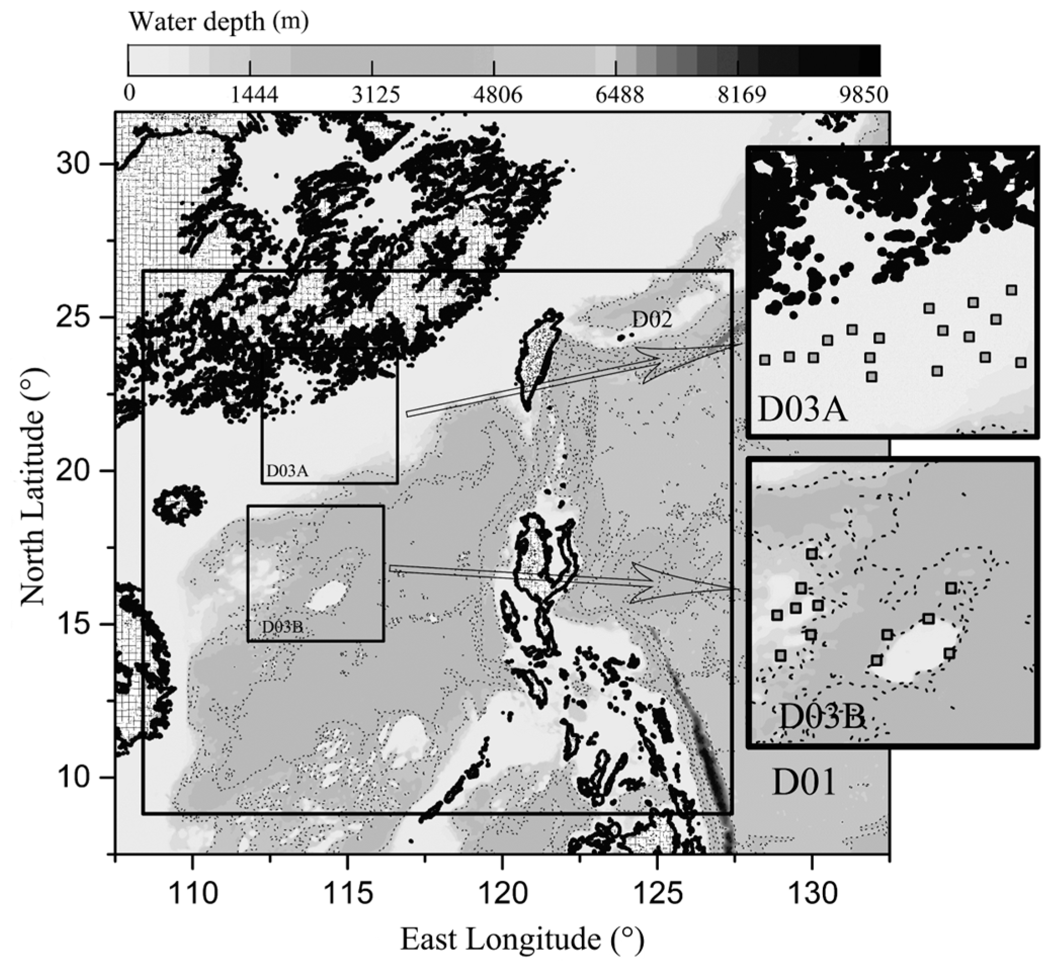
It is reasonable to assume that the water-depth has appreciable impact on the validity of the JONSWAP spectrum model and the values of its key parameters. Therefore, the wave spectra outputs from the SWAN simulation are binned according to the water-depth with a step size of 50   m ( 50   m 100   m , 100   m 150   m , 150   m 200   m , 200   m 250   m , and 250   m 300   m ) to explore the impact of the water-depth.
By fitting the simulated wave spectra extracted from the SWAN simulation to the universal form of the JONSWAP spectrum model (Equation (3)), the key parameters α and γ are derived. Afterwards, the comparison between the derived α and γ to the estimations calculated according to Equations (18)–(27) shows the values of the key parameters of the JONSWAP spectrum applicable to describe the wave characteristics found in the South China Sea. In terms of fitting the simulated wave spectra to the JONSWAP spectrum model, the Levenberg-Marquardt algorithm [47,
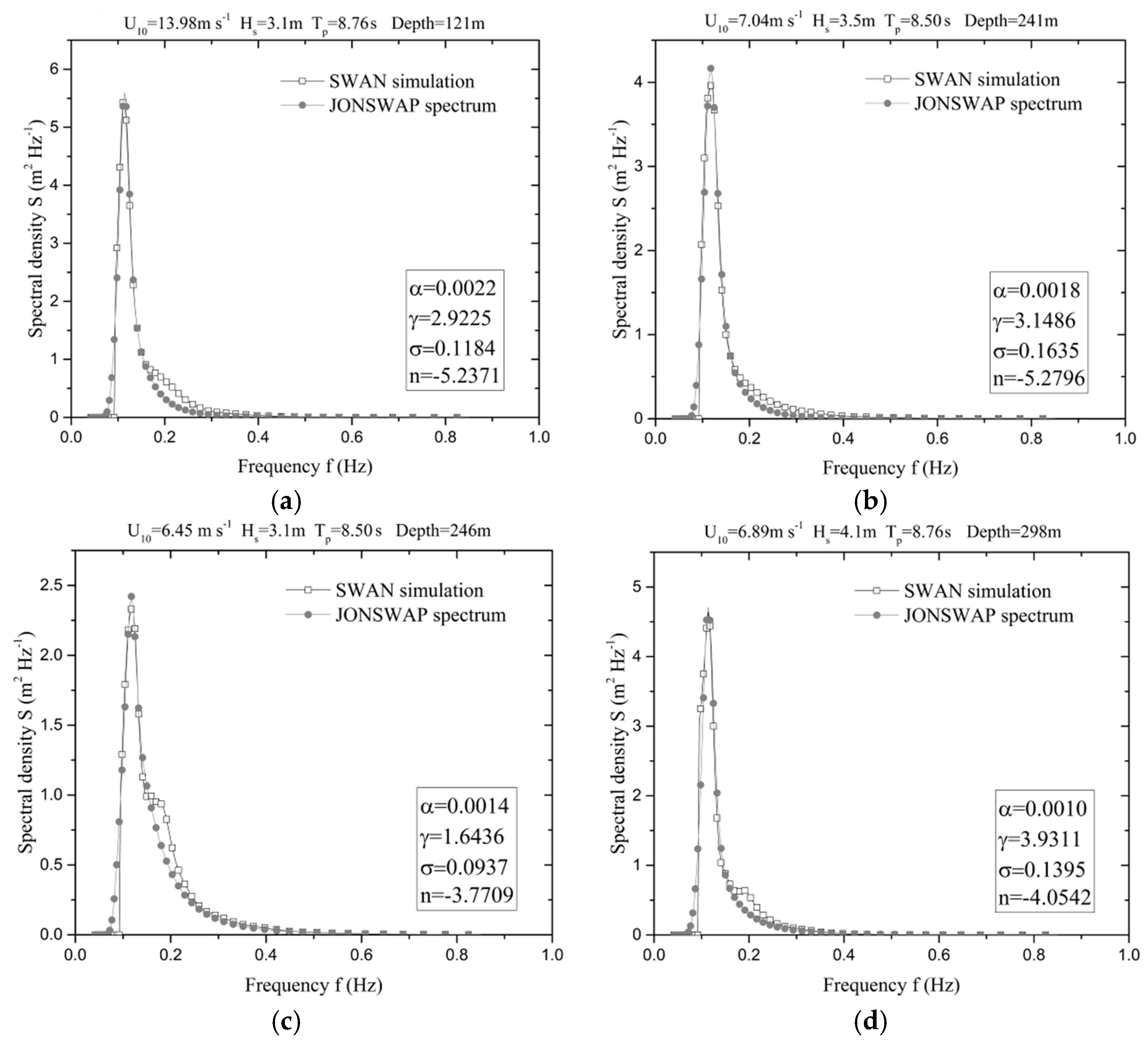
48] is adopted to solve the nonlinear least squares problem. Several fitting results are shown in Figure 5 to illustrate the feasibility of using the JONSWAP spectrum, with best-fitted key parameters, to model the wave spectra extracted from the SWAN simulation results. From Figure 5, it is discerned that the JONSWAP spectrum approaches the SWAN simulation results by adjusting the four parameters ( α , γ , σ and n ) under both typhoon and non-typhoon conditions.

4.2. Typhoon Condition

Before systematically comparing the key parameters of the JONSWAP spectrum ( α and γ ) derived from fitting the SWAN simulation results and estimated according Equations (18)–(27), it is worthwhile to examine the evolution of the wave spectra in the approach of a typhoon. 
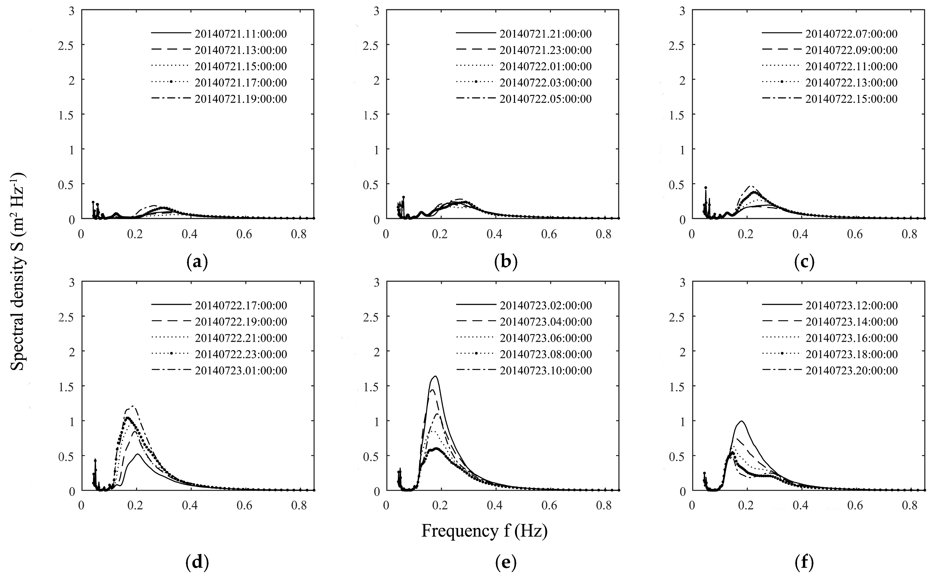
Figure 6 presents the SWAN simulated wave spectra at the position of the Wankou buoy during the passage of Typhoon Matmo. A clear increasing-decreasing trend is observed from Figure 6. More specifically, the wave spectral density in Figure 6 increases when the Typhoon Matmo approaches the position of the Wankou buoy and reaches the peak at 02:00 (UTC) on 23 July. At the peak, the Hs, T 01 , and spectral density reaches   1.80   m , 5.55   s ,   and 1.69   m 2 · Hz 1 respectively. Afterwards, the strong wind field of Typhoon Matmo swept the Wankou buoy and moved northwards, which leads to the decrease of the wave spectral density. Actually, the wave spectral density reduces to the normal level at 07:00 (UTC) on 23 July. The simulated wave spectra corresponding to other typhoons are similar in shapes as shown in Figure 6, and therefore are omitted for brevity.
In the increasing-decreasing trend shown in Figure 6, two peaks appear in the wave spectral density curves, which implies co-existing wind-induced waves and swells. When the Typhoon Matmo approaches, the peak corresponding to the wind-induced wave becomes prominent when compared to the swell peak. In fact, the swell height reaches 0.2   m at 02:00 (UTC) on 23 July, which only takes 9.82 % of the total wave energy. Such findings are in line with the conclusions derived by previous scholars. Young [16] indicated that within the radius of eight times the RMW (radius to the maximum wind) of a typhoon wind field, the uni-modal spectrum occurs in most cases. Other researches concurred that the wave fields under the influence of typhoons are commonly uni-modal and the wind-induced wave dominates the wave energy. In fact, previous scholars concluded that the wind-induced wave leads to an essentially uni-modal wave-spectrum when the Hs varies from 2   m   to   5   m [26], the wind speed exceeds 9.3   m · s 1 [49], or the root-mean-squared wave height exceeds 0.5   m [27]. In the present study, the uni-modal spectra occur in most cases when the value of Hs exceeds 2   m under typhoon condition. Consequently, the Hs is used as an indicator to identify if a certain wave spectrum output from the SWAN model is under typhoon influence. Among 4796 wave spectra derived from the SWAN simulation of typhoon cases, only 1524 spectra corresponding to the Hs larger than 2.5   m were selected for further investigations.
By analyzing the Hs and Tp of the selected 1524 wave spectra, it was found that the water-depth has appreciable impacts on the spectral characteristics of waves induced by typhoon winds. In fact, both the Hs and Tp increase with the water-depth. One plausible explanation is that the dissipation of wave energies caused by bottom frictions and waver breakings decreases in deeper waters. In order to investigate the influence of the water-depth on the wave spectra in a more systematic way, the key parameters of the JONSWAP spectrum ( α , γ , σ , and n ) derived from fitting the SWAN simulated spectra, corresponding to different water-depth bins, are presented in Table 10. It is evident from the table that α decreases with the increasing water-depth under typhoon condition. In general, n appears lower than traditional values varying from 3   to   6 , which indicates the meteorological condition (higher wind speed and larger wind fetch) keep n into a lower range around ~ 6.9 . The variation of n is not obvious with water depth ranging from 50   m to 300   m . Kumar et al. [26] concluded that the water-depth does not have significant impact on the high frequency tail decay parameter n when the water-depth is in the range of 12 70   m . The variation of n revealed in Table 10 supports such a conclusion as the value of n stays around a constant of 6.9 for the waves in the South China Sea under typhoon influence. Similarly, it has been found that the water-depth has negligible influence on the values of γ and σ , which substantiates that the water-depth and typhoon environment have a weak influence on the shape of wave spectra [21]. On the basis of above analyses, among the key parameters shaping the JONSWAP spectrum, only the Phillips constant α , representing the magnitude of the total wave energy, is necessary to be adjusted according to the water depth. In terms of using the JONSWAP spectrum model in the design of offshore wind turbines, designers and engineers are suggested to refer to Table 10 for a crude estimation.
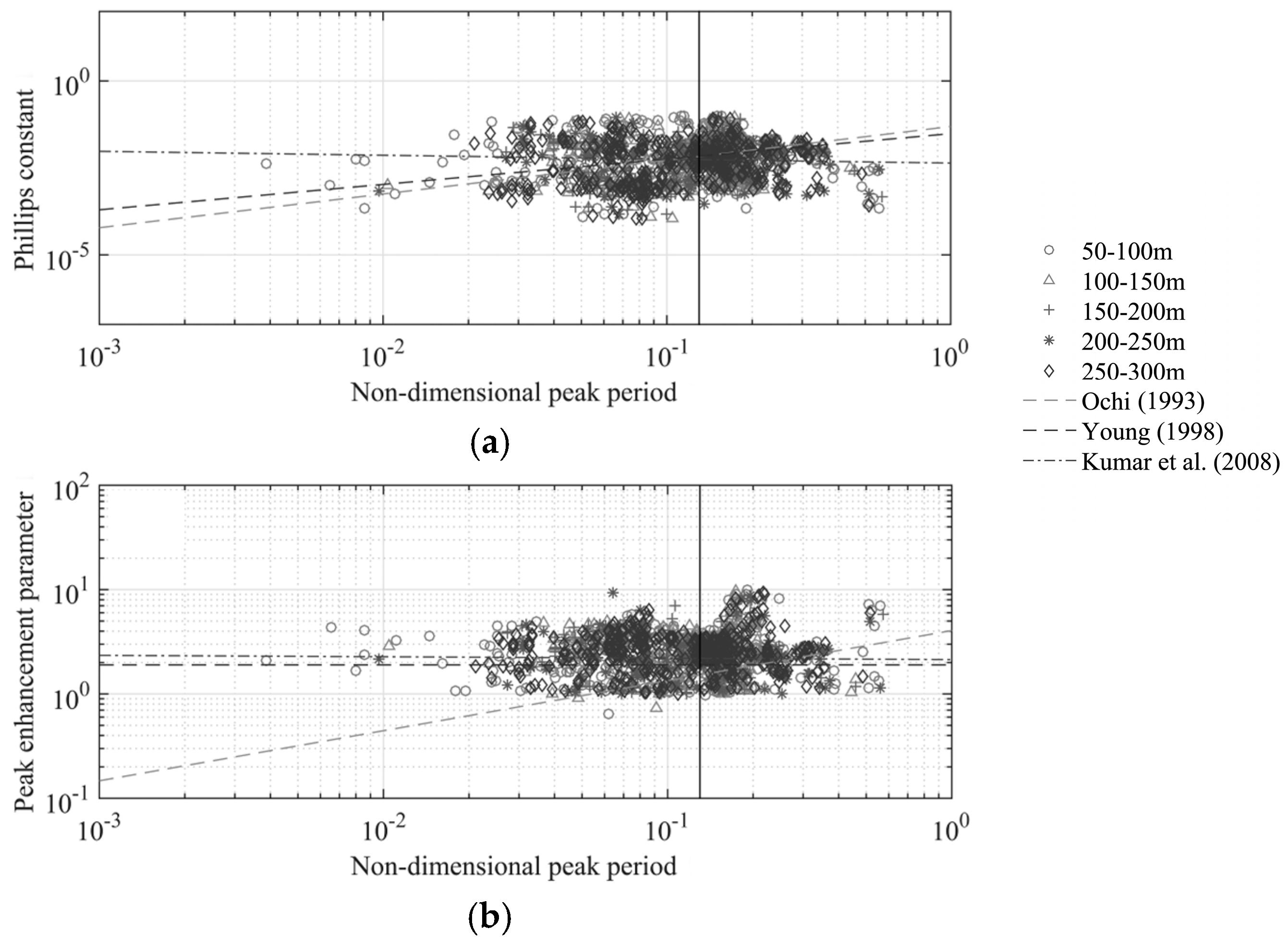
In terms of the variation of α with the υ , Figure 7a presents the results from fitting the SWAN simulated wave spectra to the JONSWAP spectrum model and the estimations made according to the equations provided in literatures. It should be noted that, υ less than 0.13 means that the propagation speed of waves at the peak frequency is faster than the local wind speed. In such case, the wave energy is not input from local winds but mainly from swells. Therefore, the black vertical lines shown in Figure 7, Figures 9 and 10 represent the boundary separating the wind-induced and swell-dominated waves. It is clear from Figure 7a that, expect for Equation (22) provided by Kumar et al. (2008) [26], Equations (18) and (20) proposed by Ochi (1993) [23] and Young (1998) [16] yield reasonable estimates of α given the υ . Similar to Figure 7a, the variation of γ with υ is plotted in Figure 7b. It is evident that significant dispersions appear in the figure, which is also recorded by previous scholars, revealing that γ only weakly depends on wave periods [18]. In fact, Young suggested to model γ as a constant of 1.9 under typhoon influences in response to the scattering of γ observed in different cases.
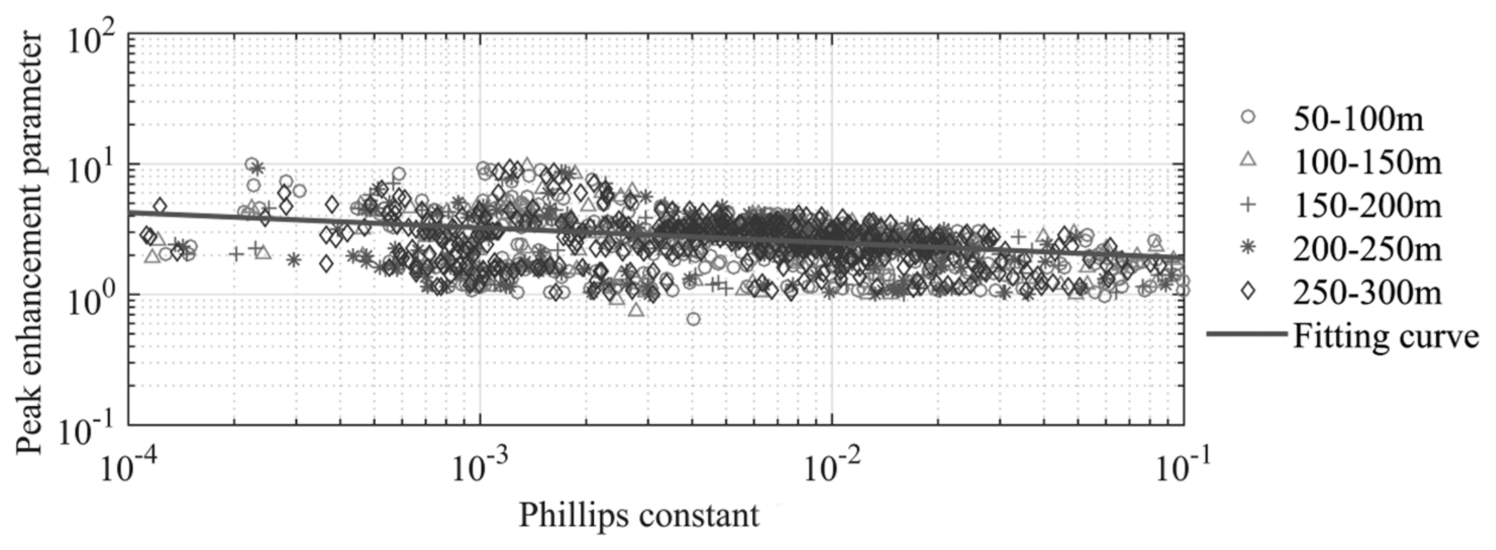
In analyzing the variations of α and γ with υ , however, it has been found that an approximate linear relation exists between α and ln ( γ ) . In fact, it seems that ln ( γ ) linearly decreases with increasing α , as shown in Figure 8. The straight line shown in Figure 8 indicates the linear regression results, which can be expressed as:
γ = 1.46 α 0.12
In summary, it is suggested that Equations (18) and (20) proposed by Ochi (1993) [23] or Young (1998) [16] are adequate to estimate α for the waves in the South China Sea under typhoon influences.
To provide a crude estimation of α for engineering application, designers and engineers are suggested to look for α according to the water-depth in Table 10. The estimation of γ , on the other hand, should be based on its relation with α as shown in Equation (28). As regards the values of σ and n , two constants are suggested ( 0.06 and 6.9 , respectively). By comparing the maximum spectral density and spectral zero moment of the wave spectra derived from the SWAN simulation and calculating according to the JONSWAP spectrum model using the parameters proposed by previous scholars and in the present study, the suggestions made above are evaluated. Table 11 presents the RMSE and Bias of the maximum spectral densities and spectral zero moments calculated differently. It is evident from the table that all the estimations yield reasonable results in terms of the maximum spectral density. As for the spectral zero moment, the estimations made according to the suggestion given in the present study outperform all other estimations to produce the lowest RMSE ( 166.55 ) and Bias ( 17.82 ).

4.3. Non-Typhoon Condition

Because the JONSWAP model is only suitable for describing the uni-modal spectrum, discussing the values of its key parameters based on fitting bi-modal spectra to the JONSWAP model is pointless. Therefore, it is necessary to rule out the bi-modal spectra from the SWAN simulation results. Comparing to the waves under typhoon conditions, the variation of Hs under non-typhoon condition has a narrower range from 0   m to 4.5   m , and the shape of wave spectra is not tightly related to the Hs as in the typhoon case. Therefore, it is not feasible to identify the uni-modal spectrum according solely to the Hs in the non-typhoon case. A simple algorithm is then designed to pick out the spectral shapes with one extreme point based on the fact that uni-model wave spectrum has the sole peak. Through screening, 14 , 306 uni-model spectra are selected from 17 , 980 wave spectra output from the SWAN simulation. Using also the Levenberg-Marquardt algorithm, the selected spectra are fitted to the JONSWAP spectrum model. The same as in the discussion on the typhoon cases, the key parameters of α , γ , σ and n are derived from the fitting process. The derived parameters are summarized in Table 12.
Comparing to the variation of α for typhoon cases in Table 10, the constant of 0.0034 shown in the column of α in Table 12 reflects the constant wave energy in the calm sea state, which implies that a constant α is adequate to yield appropriate JONSWAP spectrum for different water-depths. In fact, other parameters ( γ , σ and n ) also relatively keep constant (as 2.5 ,   0.12 and 3.9 , respectively) when the water-depth varies. Such a finding indicates that the water-depth has negligible influence on the shape of the wave spectrum under the non-typhoon condition. It is argued that the stable spectral shape is a result of relatively constant wind energy input and the weak dissipations caused by water breakings and bottom frictions. Furthermore, the values of σ and n are different from those under the typhoon condition. More specifically, σ reaches 0.12 implying a wider peak in the wave spectrum when comparing with the value of 0.06 under the typhoon condition, similar to the results from the work of Young and Verhagen [24]. n , on the other hand, keeps a larger value ( ~ 3.9 ), which is close to the modified value of 4.0 by Donelan et al. [15].
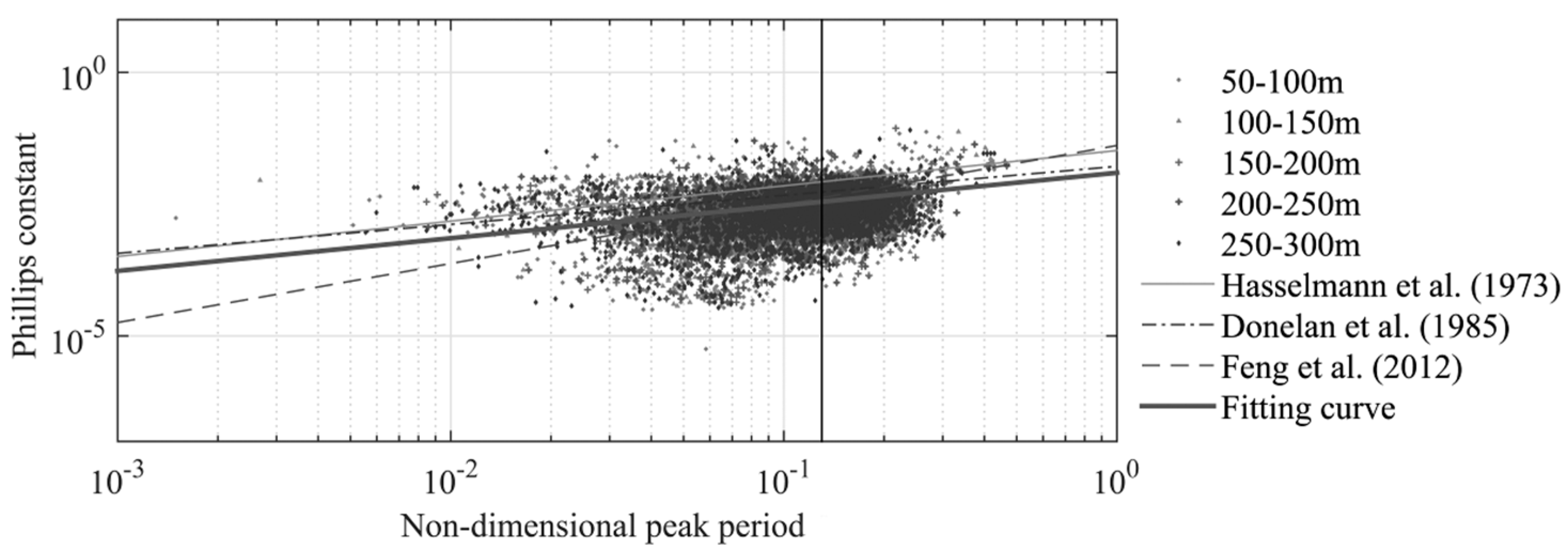
As regards the variations of α and γ with the υ , Figure 9 and Figure 10 show the values derived from the SWAN simulation results and estimated according to the equations proposed in literatures.
It has been discerned from the figure that different Equations (18)–(27) yield similar estimates, in the sense of approximating the values derived from the fitting process. In fact, the equations provided in literatures all take the form of:
α = k υ a
Their differences concern only the model constants of k and a . By fitting the derived α and calculated υ to Equation (29), the best fitted values of k and a are suggested in the present study as, k = 0.012 and a = 0.62 . Combining with Equation (15), it is suggested, based on the results of the present study, that α can be estimated as:
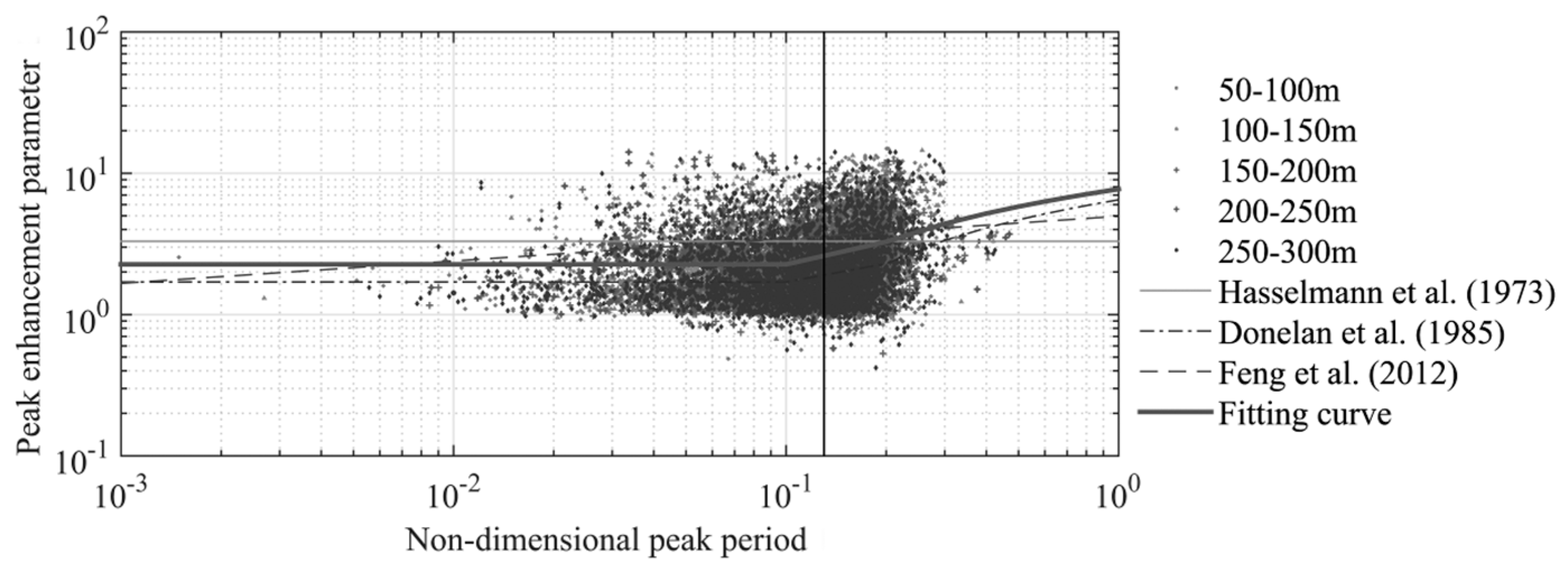
α = 0.012 [ U 10 / ( g T p ) ] 0.62
Similarly, Figure 9 and Figure 10 show the values of γ calculated based on the SWAN simulation results and estimated using the equations provided in literatures (Equations (18)–(27)). From the figure, a slight increasing trend is found when examining the variation of γ with υ . While Hasselmann et al. [11] modeled γ as a constant of 3.3 based on their observation, the piecewise function proposed by Donelan et al. [15] is found more applicable to describe the slight increasing trend of γ observed in Figure 10. Adapted from the formula proposed by Donelan et al. [15], it is suggested that γ can be expressed as a piecewise function of υ as:
γ = { 7.7218 + 6.3624 log υ , υ 0.159 2.2661 , υ < 0.159
As regards the values of σ and n , two constants ( 0.12 and 3.9 , respectively) are suggested based on examining the values derived from the fitting process.
In summary, Equations (30) and (31), and two constants are suggested in the present study to model the key parameters of the JONSWAP spectrum ( α , γ , σ and n ) in order to make it applicable to describe wave characteristics in the South China Sea under non-typhoon condition. As in the investigation concerning the typhoon case, the maximum spectral densities and spectral zero moments calculated based on the SWAN-simulated wave spectra and the JONSWAP spectrum model with the key parameters estimated using different methods are compared in Table 13.
It is clear from the table that the estimations of the key parameters proposed in the present study produce the lowest RMSE and Bias, indicating that the JONSWAP spectrum model should be revised as suggested in the present study to be applicable for describing wave characteristics in the South China Sea.

5. Conclusions

By numerically simulating the wave fields at several potential sites for constructing floating wind farms in the South China Sea, the present paper investigated the applicability of the JONSWAP spectrum model in terms of describing the wave spectral characteristics in the South China Sea under typhoon and non-typhoon conditions.
A summary covering all the key parameters of the JONSWAP spectrum model suggested in present work is listed as follows:
(a)
Group 1 (corresponding to the typhoon situation)
  • Phillips constant α
    Ochi’s (1993) equation [23]:
    4.5 H s 2 f p 4
    Young’s (1998) equation [16]:
    0.008 ( U 10 / C p ) 0.73
  • Peak-enhancement factor γ :
    γ = 1.46 α 0.12
  • Dimensionless spectral width parameter σ :
    σ = 0.06
  • High frequency decay:
    n = −6.9
(b)
Group 2 (Corresponding to the non-typhoon situation)
  • Phillips constant α :
    α = 0.012 [ U 10 / ( g T p ) ] 0.62
  • Peak-enhancement factor γ :
    γ = { 7.7218 + 6.3624 log [ U 10 / ( g T p ) ] , U 10 / ( g T p ) 0.159 2.2661 , U 10 / ( g T p ) < 0.159
  • Dimensionless spectral width parameter σ :
    σ = 0.12
  • High frequency decay:
    n = −3.9
In detail, for wave spectra under the typhoon condition, the estimations (Equations (18) and (20)) have been found adequate to show the variation of α with the υ . For crude estimation, Table 10 implies that α could be a function of the water-depth. After α has been estimated, the value of γ is suggested to be calculated using Equation (28). As for the values of σ and n , two constants ( 0.06 and 6.9 ) are suggested, which are different from the traditional values proposed by previous scholars. Such a finding indicates that the key parameters of the JONSWAP spectrum model derived based on the observations obtained elsewhere should be revised before the model can be applied to estimate the wave loads acting on the floating wind turbines erected in the South China Sea.
For wave spectra under the non-typhoon condition, a formula adapted from the conventional equation proposed in literatures is suggested to estimate α based on the υ (Equation (30)), and γ is suggested to be calculated as a piecewise function of υ (Equation (31)). Similar as in the typhoon case, two constants of 0.12 and 3.9 are suggested to model σ and n . When comparing to the values suggested by previous scholars, the results given in the present paper are more in line with the validated numerical simulation of wave fields in the South China Sea.

Acknowledgments

The authors would like to express their gratitude towards following organizations for financially supporting the work described in the present paper, which includes the economy, trade and Information Commission of Shenzhen Municipality (Project Nos. 201510150880 and SZHY2014-B01-001) and National Natural Science Foundation of China (Project No. 51608302).

Author Contributions

Sunwei Li and Yichao Liu conceived and designed the simulation schemes and procedures; Yichao Liu conducted the simulations; Yichao Liu and Qian Yi analyzed the data; Daoyi Chen guided the research and contributed the necessary tools; Sunwei Li and Yichao Liu wrote the paper.

Conflicts of Interest

The authors declare no conflict of interest.

References

  1. Aiming High Rewarding Ambition in Wind Energy; European Wind Energy Association (EWEA) Business Intelligence: Brussels, Belgium, 2015.
  2. Failla, G.; Arena, F. New perspectives in offshore wind energy. Philos. Trans. R. Soc. Lond. A Math. Phys. Eng. Sci. 2015, 373. [Google Scholar] [CrossRef] [PubMed]
  3. Liu, Y.; Li, S.; Yi, Q.; Chen, D. Developments in semi-submersible floating foundations supporting wind turbines: A comprehensive review. Renew. Sustain. Energy Rev. 2016, 60, 433–449. [Google Scholar] [CrossRef]
  4. Zheng, C.; Zhuang, H.; Li, X.; Li, X. Wind energy and wave energy resources assessment in the East China Sea and South China Sea. Sci. China Technol. Sci. 2011, 55, 163–173. [Google Scholar] [CrossRef]
  5. Douglas, P.H. The development of a system of federal grants-in-aid II. Political Sci. Q. 1920, 35, 522–544. [Google Scholar] [CrossRef]
  6. Liang, S.X.; Sun, Z.C.; Yin, H.Q.; Niu, H.Y. Influence factors of typhoon wave forecast in the South Sea by SWAN model. Adv. Mar. Sci. 2015, 1, 19–30. (In Chinese) [Google Scholar]
  7. Morison, J.; Johnson, J.; Schaaf, S. The force exerted by surface waves on piles. J. Pet. Technol. 1950, 2, 149–154. [Google Scholar] [CrossRef]
  8. Faltinsen, O. Wave loads on offshore structures. Annu. Rev. Fluid Mech. 1990, 22, 35–56. [Google Scholar] [CrossRef]
  9. Roddier, D.; Cermelli, C.; Aubault, A.; Weinstein, A. WindFloat: A floating foundation for offshore wind turbines. J. Renew. Sustain. Energy 2010, 2, 033104. [Google Scholar] [CrossRef]
  10. Mayilvahanan, A.; Selvam, R. Time Domain Response Analysis of Barge Floater Supporting an Offshore Wind Turbine. Int. J. Ocean Clim. Syst. 2011, 2, 303–314. [Google Scholar] [CrossRef]
  11. Hasselmann, K.; Barnett, T.; Bouws, E.; Carlson, H.; Cartwright, D.; Enke, K.; Ewing, J.; Gienapp, H.; Hasselmann, D.; Kruseman, P. Measurements of Wind-Wave Growth and Swell Decay during the Joint North Sea Wave Project (JONSWAP); Deutches Hydrographisches Institut: Hamburg, Germany, 1973. [Google Scholar]
  12. Pierson, W.J., Jr.; Moskowitz, L. A proposed Spectral Form for Fully Developed Wind Seas Based on the Similarity Theory of SA Kitaigorodskii; DTIC Document: Fort Belvoir, VA, USA, 1963. [Google Scholar]
  13. Stormy Weather in the North Sea; National Aeronautics and Space Administration: Washington, DC, USA, 2006.
  14. Toba, Y. Local Balance in the Air-Sea Boundary Processes: I. On the Growth Process of Wind Waves. J. Oceanogr. Soc. Jpn. 1972, 28, 109–120. [Google Scholar] [CrossRef]
  15. Donelan, M.A.; Hamilton, J.; Hui, W.H. Directional spectra of wind-generated waves. Philos. Trans. R. Soc. Lond. A Math. Phys. Eng. Sci. 1985, 315, 509–562. [Google Scholar] [CrossRef]
  16. Young, I. Observations of the spectra of hurricane generated waves. Ocean Eng. 1998, 25, 261–276. [Google Scholar] [CrossRef]
  17. Forristall, G.Z. Measurements of a saturated range in ocean wave spectra. J. Geophys. Res. Atmos. 1981, 86, 8075–8084. [Google Scholar] [CrossRef]
  18. Young, I.; Verhagen, L. The growth of fetch limited waves in water of finite depth. Part 2. Spectral evolution. Coast. Eng. 1996, 29, 79–99. [Google Scholar] [CrossRef]
  19. Lewis, A.; Allos, R. JONSWAP’s parameters: Sorting out the inconsistencies. Ocean Eng. 1990, 17, 409–415. [Google Scholar] [CrossRef]
  20. Akpınar, A.; van Vledder, G.P.; Kömürcü, M.İ.; Özger, M. Evaluation of the numerical wave model (SWAN) for wave simulation in the Black Sea. Cont. Shelf Res. 2012, 50, 80–99. [Google Scholar] [CrossRef]
  21. Young, I. A review of the sea state generated by hurricanes. Mar. Struct. 2003, 16, 201–218. [Google Scholar] [CrossRef]
  22. Ochi, M.K.; Hubble, E.N. Six-parameter wave spectra. In Proceedings of the 15th International Conference on Coastal Engineering, Honolulu, HI, USA, 11–17 July 1976.
  23. Ochi, M.K. On Hurricane-Generated Seas. In Proceedings of the Second International Symposium on Ocean Wave Measurement and Analysis, New Orleans, LA, USA, 25–28 July 1993.
  24. Young, I.; Verhagen, L. Fetch limited spectral evolution in finite depth water. Coast. Eng. 1996, 1, 516–526. [Google Scholar]
  25. Chakrabarti, S. Handbook of Offshore Engineering (2-Volume Set); Elsevier: Amsterdam, The Netherlands, 2005. [Google Scholar]
  26. Kumar, V.S.; Kumar, K.A. Spectral characteristics of high shallow water waves. Ocean Eng. 2008, 35, 900–911. [Google Scholar] [CrossRef]
  27. Feng, W.B.; Yang, B.; Cao, H.J.; Ni, X.Y. Study on Wave Spectra in South Coastal Waters of Jiangsu. Appl. Mech. Mater. 2012, 212–213, 193–200. [Google Scholar] [CrossRef]
  28. Booij, N.; Holthuijsen, L.; Ris, R. The “SWAN” wave model for shallow water. In Proceedings of the 25th Conference on Coastal Engineering, Orlando, FL, USA, 14–19 July 1996.
  29. Ris, R.; Holthuijsen, L.; Booij, N. A third-generation wave model for coastal regions: 2. Verification. J. Geophys. Res. 1999, 104, 7667–7681. [Google Scholar] [CrossRef]
  30. Whitham, G.B. Linear and Nonlinear Waves; John Wiley & Sons: Hoboken, NJ, USA, 2011; Volume 42. [Google Scholar]
  31. Cavaleri, L.; Alves, J.H.; Ardhuin, F.; Babanin, A.; Banner, M.; Belibassakis, K.; Benoit, M.; Donelan, M.; Groeneweg, J.; Herbers, T.H.C. Wave Modeling—The State of the Art. Prog. Oceanogr. 2007, 74, 603–674. [Google Scholar] [CrossRef] [Green Version]
  32. Booij, N.; Haagsma, J.; Van der Westhuysen, A. Swan User Manual; Delft University of Technology: Delft, The Netherlands, 2004; pp. 1–11. [Google Scholar]
  33. Scientific and Technical Documentation SWAN Cycle 3 Version 41.01AB; The SWAN Team: Delft, The Netherlands, 2015.
  34. Zijlema, M.; van Vledder, G.P.; Holthuijsen, L. Bottom friction and wind drag for wave models. Coast. Eng. 2012, 65, 19–26. [Google Scholar] [CrossRef]
  35. Pallares, E.; Sánchez-Arcilla, A.; Espino, M. Wave energy balance in wave models (SWAN) for semi-enclosed domains—Application to the Catalan coast. Continent. Shelf Res. 2014, 87, 41–53. [Google Scholar] [CrossRef]
  36. Cavaleri, L.; Rizzoli, P.M. Wind wave prediction in shallow water: Theory and applications. J. Geophys. Res. Oceans 1981, 86, 10961–10973. [Google Scholar] [CrossRef]
  37. Tolman, H.L.; Accensi, M.; Alves, H.; Ardhuin, F.; Bidlot, J.; Booij, N.; Bennis, A.-C.; Campbell, T.; Chalikov, D.V.; Filipot, J.-F. User Manual and System Documentation of Wavewatch III Version 4.18. 2014. Available online: http://polar.ncep.noaa.gov/waves/wavewatch/manual.v4.18.pdf (accessed on 3 January 2017). [Google Scholar]
  38. Komen, G.; Hasselmann, K.; Hasselmann, K. On the existence of a fully developed wind-sea spectrum. J. Phys. Oceanogr. 1984, 14, 1271–1285. [Google Scholar] [CrossRef]
  39. Battjes, J.; Janssen, J. Energy loss and set-up due to breaking of random waves. In Proceedings of the 16th International Conference on Coastal Engineering, Hamburg, Germany, 27 August–3 September 1978.
  40. Eldeberky, Y.; Battjes, J.A. Spectral modeling of wave breaking: Application to Boussinesq equations. J. Geophys. Res 1996, 101, 1253–1264. [Google Scholar] [CrossRef]
  41. Hasselmann, S.; Hasselmann, K.; Allender, J.; Barnett, T. Computations and parameterizations of the nonlinear energy transfer in a gravity-wave specturm. Part II: Parameterizations of the nonlinear energy transfer for application in wave models. J. Phys. Oceanogr. 1985, 15, 1378–1391. [Google Scholar] [CrossRef]
  42. RA IV Hurricane Committee. Regional Association IV Hurricane Operational Plan 2015; World Meteorological Organization: Geneva, Switzerlands, 2015. [Google Scholar]
  43. State Oceanic Administration. Specifications for Oceanographic Survey Part 3: Marine Meteorological Observations; (GB/T12763.3-2007/8); Standards Press of China: Beijing, China, 2007. [Google Scholar]
  44. Lin, W.; Sanford, L.P.; Suttles, S.E. Wave measurement and modeling in Chesapeake Bay. Cont. Shelf Res. 2002, 22, 2673–2686. [Google Scholar] [CrossRef]
  45. Liu, P.C.; Schwab, D.J.; Jensen, R.E. Has wind–wave modeling reached its limit? Ocean Eng. 2002, 29, 81–98. [Google Scholar] [CrossRef]
  46. Li, R.L. On the relationships of various wind wave periods. Trans. Oceanol. Limnol. 2007, 2, 13–18. (In Chinese) [Google Scholar]
  47. Levenberg, K. A method for the solution of certain non–linear problems in least squares. Q. Appl. Math. 1944, 2, 164–168. [Google Scholar] [CrossRef]
  48. Marquardt, D.W. An algorithm for least-squares estimation of nonlinear parameters. J. Soc. Ind. Appl. Math. 1963, 11, 431–441. [Google Scholar] [CrossRef]
  49. Pan, Y.P.; Ge, S.F.; Sha, W.Y.; Shen, S.H. An analysis on the statistical characteristic of sea waves with double-peaked spectrum. Acta Oceanol. Sin. 2009, 31, 13–21. (In Chinese) [Google Scholar]
Figure 1. The simulating waves nearshore (SWAN) domain configuration shown on top of the hydrology map of the South China Sea. Twenty nine potential floating wind farm sites are indicated by small squares.
Energies 10 00127 g001
Figure 2. Comparisons between observed and simulated Hs and T 01 15–18 July, 20–24 July and 12–18 September in 2014: (a) Hs in Typhoon Rammasun; (b) T 01 in Typhoon Rammasun; (c) Hs in Typhoon Matmo; (d) T 01 in Typhoon Matmo; (e) Hs in Typhoon Kalmaegi; and (f) T 01 in Typhoon Kalmaegi.
Energies 10 00127 g002
Figure 3. Comparisons between observed and simulated Hs and T 01 at buoy sites under normal conditions: (a) Hs from 1 to 8 April 2014; (b) T 01 from 1 to 8 April 2014; (c) Hs from 29 August to 5 September 2014; and (d) T 01 from 29 August to 5 September 2014. The solid lines represent the perfectly-matching curve while the dashed lines showing the reliable region of the buoy measurements ( ± 0.1   m ).
Energies 10 00127 g003
Figure 4. The error indicators in the normal days (1999–2013).
Energies 10 00127 g004
Figure 5. The comparison between wave spectra generated by SWAN simulation and calculations according to the JONSWAP spectrum model (with best-fitted parameters). Water depth: (a) 121 m; (b) 241 m; (c) 246 m; and (d) 298 m.
Energies 10 00127 g005
Figure 6. SWAN simulated wave spectra at Wankou buoy position during the passage of Typhoon Matmo from 21 to 23 July 2014: (a) from 11:00, 21 July 2014 to 19:00, 21 July 2014; (b) from 21:00, 21 July 2014 to 05:00, 22 July 2014; (c) from 07:00, 22 July 2014 to 15:00, 22 July 2014; (d) from 17:00, 22 July 2014 to 01:00, 23 July 2014; (e) from 02:00, 23 July 2014 to 10:00, 23 July 2014; and (f) from 12:00, 23 July 2014 to 20:00, 23 July 2014.
Energies 10 00127 g006
Figure 7. Values of α and γ as functions of υ for the 3 typhoon simulations. The empirical Equations (18)–(23) by Ochi (1993) [23], Young (1998) [16] and Kumar (2008) [26] are shown. The vertical line drawn at υ = 0.13 marks the commonly adopted boundary separating swell-dominated and wind-induced waves: (a) the relation between α and υ ; and (b) the relation between γ and υ .
Energies 10 00127 g007
Figure 8. Values of ln ( γ ) as a function of α .
Energies 10 00127 g008
Figure 9. Values of as a function of υ for normal condition from 1999 to 2014. Three empirical Equations (4), (24) and (26) by Hasselmann (1973) [11], Donelan et al. [15] and Feng et al., (2012) [27] are shown. The vertical line drawn at υ = 0.13 marks the commonly adopted boundary between swell and wind wave.
Energies 10 00127 g009
Figure 10. Values of γ as a function of ν for normal condition from 1999 to 2014. The average 3.3 and 2 empirical Equations (24) and (26) proposed by Hasselmann (1973) [11], Donelan et al., (1985) [15] and Feng et al., (2012) [27] are shown. The vertical line drawn at υ = 0.13 marks the commonly adopted boundary between swell and wind wave.
Energies 10 00127 g010
Table 1. Phillips constant, peak-enhancement factor and dimensionless spectral width parameter proposed in previous literatures. Hs: significant wave height; Fp: peak frequency; T02: zero-crossing mean wave period; Cp: phase speed of components at the spectral peak frequency; D: non-dimensional fetch.
AuthorsPhillips Constant αPeak-Enhancement Factor γDimensionless Spectral Width Parameter σ
Hasselmann (1973) [11] α = 0.076 D 0.22 3.3 σ = { 0.07 , f < f p 0.09 , f f p
Ochi and Hubble (1976) [22] 0.0023 2.2 -
Donelan et al. (1985) [15] 0.006 ( U 10 / C p ) 0.55 { 1.7 + 6 log 10 ( U 10 / C p ) , U 10 / C p 0.159 1.7 , U 10 / C p < 0.159 -
Ochi (1993) [23] 4.5 H s 2 f p 4 9.5 H s 0.34 f p -
Young and Verhagen (1996) [24]--0.12
Young (1998) [16] 0.008 ( U 10 / C p ) 0.73 1.90.1
Chakrabarti (2005) [25] 5.058 ( H s T p 2 ) 2 ( 1 0.287 ln γ ) { γ = 5 , for   T p / H s 3.6 γ = exp ( 5.75 1.15 T p / H s ) , for   T p / H s > 3.6 -
Kumar et al. (2008) [26] 0.18 H s 1.52 T P 3.53 T 02 1.34 8.38 H s 0.57 T p 1.26 T 02 0.41 -
Feng et al. (2012) [27] 4.069 H s 2.06 T p 4.24 6.236 H s 0.12 T p 0.34 -
Table 2. The statistics of wave information with the varying incoming Hs. Hwell: wave spectrum.
Incoming Hs (m)Hs (m)Hwell (m) T 02 (s)
Minimum/Average/Maximum
10.6240/1.7325/5.49910/0.9803/5.38952.4776/6.3609/13.6666
30.6240/1.7324/5.50200/0.9803/5.38802.4776/6.3622/13.6505
50.6240/1.7330/5.50430/0.9804/5.38992.4776/6.3565/13.6530
70.6240/1.7326/5.50340/0.9805/5.39002.4776/6.3615/13.6639
90.6240/1.7325/5.49820/0.9804/5.38612.4776/6.3622/13.6623
Table 3. Detailed settings of the SWAN model. LTA: lumped triad approximation.
SWAN SimulationD01D02D03A and D03B
Basic settings
Grid points 98 × 98 222 × 219 165 × 165
No. of frequencies100100100
No. of directions363636
Time step30 min30 min10 min
Mode
Linear wave growthCavaleri and Malanotte-Rizzoli [36] and Tolman et al.’s methods [37]
Exponential wave growthKomen method [38]
Physics
White cappingKomen method [38]
Bottom frictionJONSWAP scheme [11]
Depth-induced breakingBore-based model [39]
Triad wave-wave interactionLTA method [40]
Quadruplet wave-wave interactionsHasselmann method [41]
Table 4. The start and end point of the time period under typhoon conditions and non-typhoon conditions.
Start DateEnd DateCondition
15 July 201418 July 2014Typhoon Rammasun
20 July 201424 July 2014Typhoon Matmo
12 September 201418 September 2014Typhoon Kalmaegi
1 April 20148 April 2014Buoy data are available for validation
29 August 20145 September 2014
1 April 1999–20133 April 1999–2013Normal days
1 June 1999–20133 June 1999–2013
12 September 1999–201315 September 1999–2013
17 December 1999–201320 December 1999–2013
Table 5. Summary of the statistical errors for the simulations during Typhoon Rammasun process from 15 to 18 July 2014. RMSE: root mean square error; SD: standard deviation; and SI: scatter index.
ObservationsDataRMSEBiasSDSI
Dongchong Buoy H s (m)0.3750−0.01680.37460.2424
T 01 (s)1.3168−1.12000.69250.2021
Dameisha Buoy H s (m)0.27210.23370.13940.3741
T 01 (s)1.4670−1.10590.96390.2708
Xiasha Buoy H s (m)0.36570.25830.25890.5099
T 01 (s)1.3774−0.83341.09680.2470
Wankou Buoy H s (m)0.3736−0.13810.34710.2042
T 01 (s)1.2112−0.67471.00580.1472
Table 6. Summary of the statistical errors for the simulations during Typhoon Matmo process from 20 to 24 July 2014.
ObservationsDataRMSEBiasSDSI
Dongchong Buoy H s (m)0.16860.01600.16790.2673
T 01 (s)1.39390.90651.05890.2747
Dameisha Buoy H s (m)0.0856−0.04150.07490.3293
T 01 (s)0.8539−0.38560.76190.1443
Xiasha Buoy H s (m)0.14750.05720.13600.4575
T 01 (s)1.16820.64020.97720.2423
Wankou Buoy H s (m)0.06050.02240.05620.0800
T 01 (s)0.9703−0.61160.75320.1551
Table 7. Summary of the statistical errors for the simulations during Typhoon Kalmaegi process from 12 to 18 September 2014.
ObservationsDataRMSEBiasSDSI
Dongchong Buoy H s  (m)0.50550.08440.24840.3372
T 01  (s)0.77670.11560.58980.1135
Dameisha Buoy H s (m)0.11050.07990.00580.2483
T 01  (s)0.3711−0.08850.12990.0904
Xiasha Buoy H s  (m)0.05420.03550.00170.1819
T 01  (s)0.54460.32970.18790.1231
Table 8. Summary of the statistical errors for the simulations from 1 to 8 April 2014.
ObservationsDataRMSEBiasSDSI
Dameisha Buoy H s  (m)0.1277−0.04890.01390.4307
T 01  (s)1.0090−0.74080.46930.2543
Xiasha Buoy H s (m)0.06310.03400.00280.3656
T 01  (s)0.4783−0.23250.17480.1181
Table 9. Summary of the statistical errors for the simulations from 29 August to 5 September 2014.
ObservationsDataRMSEBiasSDSI
Dameisha Buoy H s (m)0.08310.02770.00610.3200
T 01 (s)0.8410−0.42780.52430.2039
Xiasha Buoy H s (m)0.06310.03400.00280.3656
T 01 (s)0.4783−0.23250.17480.1181
Table 10. JONSWAP parameters under typhoon conditions for different water depth.
Water Depth (m)Average
α γ σ n
50–1000.01182.73030.0716−6.9987
100–1500.01132.72250.0637−7.1959
150–2000.01082.82320.0675−7.0593
200–2500.00972.64120.0598−6.8065
250–3000.00962.73310.0578−6.4990
Total0.01072.71620.0638−6.8777
Table 11. The comparisons of wave energy estimation using different empirical equations under typhoon conditions.
Empirical Equations for JONSWAP Spectrum ModelMaximum Spectral EnergySpectral Zeroth Moment
RMSEBiasRMSEBias
Ochi (1993) [23]10.18190.0655294.5736114.5927
Young (1998) [16]10.02663.8791307.5289139.2901
Kumar et al. (2008) [26]10.46592.4565251.7333104.7745
Present study10.65621.2101166.546817.8185
Table 12. JONSWAP parameters under non-typhoon conditions for different water depth.
Water Depth (m)Average
α γ σ n
50–1000.00342.49920.1195−3.8890
100–1500.00342.61280.1238−3.8192
150–2000.00342.54520.1222−3.8327
200–2500.00342.45740.1191−3.9297
250–3000.00332.45020.1180−3.8783
Total0.00342.49410.1196−3.8800
Table 13. The comparisons of wave energy estimation using different empirical equations under normal conditions.
Empirical Equations for JONSWAP Spectrum ModelMaximum Spectral EnergySpectral Zeroth Moment
RMSEBiasRMSEBias
Hasselmann et al. (1973) [11]4.74752.725464.100123.9587
Donelan et al. (1985) [15]1.61780.671927.59462.2154
Feng et al. (2012) [27]1.60430.583543.087311.0258
Present study1.40670.412834.11025.7088

