Numerical Analysis of the Effects of Rotating Wind Turbine Blades on the Aerodynamic Forces Acting on Tower

Abstract

We have investigated the effects of the rotating blades of an upwind-type three-blade horizontal-axis wind turbine (HAWT) on the basic characteristics of aerodynamic forces acting on its tower by conducting improved delayed detached-eddy simulations (DESs). Three tip-speed ratios were considered for the operating conditions of the HAWT: λ = 3 (low), λ = 6 (optimum), and λ = 10 (high). The diversion of the flow approaching the tower by the rotating blades and the low-pressure region that formed downwind of the blades significantly affected the aerodynamic forces acting on the tower. For example, the azimuth angle around the tower at which the pressure reached a maximum at each height shifted significantly in the direction of the movement of the blade passing the tower because of the diversion of the flow by the blades. Fluctuations in the lift force of the tower were significantly larger than those in its drag force because of the low-pressure region downwind of the blades.

1. Introduction

When designing a wind turbine, it is important to avoid the excitation of resonant oscillations of the wind turbine tower by rotor thrust fluctuations at the blade-passing frequency or, to a lesser extent, at the rotational frequency. Wind turbine towers are customarily divided into three categories according to their stiffness: stiff, soft, and soft-soft [1,2,3]. A stiff tower is one whose fundamental natural frequency is above the blade-passing frequency range, a soft tower is one whose natural frequency is between the blade-passing frequency range and the rotor frequency range, and a soft-soft tower is one whose natural frequency is below both the rotor frequency range and the blade-passing frequency range. Because stiff towers usually require extra material not otherwise required for strength, soft towers are generally preferred. Soft and soft-soft towers can however be excited during the startup or shutdown of the turbine. In addition, dynamic magnification directly impacts the fatigue loads. Therefore, it is essential to design wind turbines and towers with the proper fatigue strength by considering their vibratory characteristics.

One of the main causes of rotor-thrust fluctuations at the blade-passing frequency is blade-tower interaction (BTI). Regardless of whether the configuration is upwind or downwind, the thrust force on the rotor of a horizontal-axis wind turbine (HAWT) decreases when a blade passes by its tower because the wind velocity of the wind approaching the tower and the wind velocity in the wake of the tower are reduced owing to the existence of the tower. The effects of the BTI on the rotor thrust have been extensively studied with computational fluid dynamics (CFD) simulations for upwind-type HAWTs [4,5,6,7,8,9,10,11] and downwind-type HAWTs [12,13]. However, studies on the effects of the BTI on the aerodynamic forces acting on the tower are very limited [11]. These studies involved CFD simulations of the National Renewable Energy Laboratory (NREL) Phase IV turbine [14] using Reynolds-averaged Navier-Stokes (RANS) turbulence models. Their main findings are as follows: Gómez-Iradi et al. [5] showed that the pressure on the upwind surface of the tower was reduced above the lowest point of the rotor at a certain rotational speed. This effect was evident even when the tips of the two blades were the maximum distance away from the tower (i.e., the angle between the tower and the blade was 90°). Wang et al. [9] reported that the pressure drop on the upwind surface of the tower, which Gómez-Iradi et al. [5] showed, was very weak at a certain tip-speed ratio when the tips of the two blades were relatively far from the tower. Using the HAWT with a downwind configuration, Zahle et al. [13] showed that the rotor had a strong effect on the tower shedding frequency, causing vortex lock-in at the upper part of the tower under certain flow conditions. They suggested the possibility that these lock-in phenomena were due to numerical artifacts of the RANS turbulence model. They also emphasized the necessity of further investigation using a large-eddy simulation (LES) or a hybrid RANS-LES model, which can reproduce separated flows more realistically.

In this study, as a first step toward clarifying the effects of aerodynamic forces acting on the tower of a wind turbine on the vibratory characteristics of the tower, we investigated the effects of the rotating blades of an upwind-type HAWT on the basic aerodynamic characteristics of the tower (e.g., the drag, lift, and pressure coefficients). This was done by conducting CFD simulations with the improved delayed detached-eddy simulation (IDDES) model [14], which is a hybrid RANS-LES model, of the wind flow around the wind turbine and its tower at low, optimum, and high tip-speed ratios.

2. Numerical Approach

In this study, a right-handed Cartesian coordinate system (x₁, x₂, x₃) = (x, y, z) is employed, in which the z-direction is aligned in the vertical direction. The CFD software utilized to simulate the wind flow field is ANSYS Fluent 17.1 (ANSYS, Inc., Canonsburg, PA, USA) [15,16].

2.1. Wind Turbine and Tower

Figure 1 shows the geometry of the wind turbine and tower investigated by the CFD simulation. The rotor and nacelle are modeled as the upwind-type HAWT used by Eriksen and Krogstad [17] and Krogstad and Eriksen [18] in their wind tunnel experiments. The diameter of the rotor is D = 0.894 m, and the center of the rotor is located 0.817 m above the floor. The blades have a non-uniform twist and chord-length distribution, and have an NREL S826 airfoil profile [19]. The tower has a uniform diameter of d = 0.061 m in the vertical direction. It is divided into 10 segments, and the aerodynamic forces acting on each segment are analyzed. The segments have identical lengths of h = 0.0772 m.

2.2. Governing Equations and Discretization Method

The detached-eddy simulation (DES) model [20] is a hybrid RANS-LES model that treats near-wall regions in a RANS-like manner, and treats the rest of the flow in an LES-like manner. This model has the potential to save a large amount of computing resources compared with a pure LES model. However, modeled-stress depletion and grid-induced separation are problems in this model. The IDDES model mitigates these effects by delaying the RANS-to-LES transition and increasing the modeled stress contribution across the interface.

The flow field around the wind turbine is assumed to be incompressible and isothermal in air at a temperature of 15 °C. The governing equations for the IDDES model are the continuity equation:

$$\frac{\partial u_i}{\partial x_i}=0$$

(1)

the Navier–Stokes equation:

$$\frac{\partial u_i}{\partial t}+\frac{\partial u_i{u}_j}{\partial x_j}=-\frac{1}{\rho }\frac{\partial p}{\partial x_i}+\nu \frac{\partial }{\partial x_j}\left(\frac{\partial u_i}{\partial x_j}+\frac{\partial u_j}{\partial x_i}-\frac{2}{3}{\delta }_{ij}\frac{\partial u_i}{\partial x_j}\right)-\frac{1}{\rho }\frac{\partial }{\partial x_j}\left[{\mu }_t\left(\frac{\partial u_i}{\partial x_j}+\frac{\partial u_j}{\partial x_i}\right)-\frac{2}{3}\rho k{\delta }_{ij}\right]$$

(2)

the transport equation for the turbulence kinetic energy k:

$$\frac{\partial k}{\partial t}+\frac{\partial k{u}_j}{\partial x_j}=\frac{\partial }{\partial x_j}\left[\left(\nu +\frac{{\mu }_t}{\rho {\sigma }_k}\right)\frac{\partial k}{\partial x_j}\right]+\frac{2{\mu }_t}{\rho }{S}_{ij}{S}_{ij}-\frac{k^{1.5}}{L_{IDDES}}$$

(3)

and the transport equation for the specific dissipation rate ω:

$$\frac{\partial \omega }{\partial t}+\frac{\partial \omega u_j}{\partial x_j}=\frac{\partial }{\partial x_j}\left[\left(\nu +\frac{{\mu }_t}{\rho {\sigma }_{\omega }}\right)\frac{\partial \omega }{\partial x_j}\right]+\left(1-F_1\right)\frac{2}{{\sigma }_{\omega }\omega }\frac{\partial k}{\partial x_j}\frac{\partial \omega }{\partial x_j}+\frac{2\alpha \omega {\mu }_t}{\rho k}{S}_{ij}{S}_{ij}-\beta {\omega }^2$$

(4)

where u_i is the wind-velocity component in the x_i direction; p is the pressure; ν is the kinematic viscosity; μ_t is the turbulence viscosity; t is the time; ρ is the air density; S_ij is the mean strain rate; L_IDDES is the IDDES length scale [14]; F₁ is a blending function [21]; σ_k and σ_ω are the turbulent Prandtl numbers for k and ω, respectively; and β is a model constant [22]. μ_t is computed as follows:

$${\mu }_t=\frac{\rho k}{\omega }\frac{1}{\max \left[\frac{1}{\alpha *},\frac{\sqrt{2S_{ij}{S}_{ij}}{F}_2}{{\alpha }_1\omega }\right]}$$

(5)

where α* is a low-Reynolds number correction coefficient [21], F₂ is a blending function [21], and α₁ is a model constant.

The governing equations are discretized by the finite-volume method. The advection terms of the Navier–Stokes equations are discretized by the bounded central-difference scheme. The advection terms of the transportation equations for k and ω are discretized by the QUICK scheme. Other spatial derivatives are discretized by the central-difference scheme. The time integration is performed using the first-order implicit method.

2.3. Numerical Setup

The computational grids, the boundary conditions, and the total number of computational cells for all run cases are shown in Figure 2 and

Table 1. Computational conditions. Here, λ is the tip-speed ratio; D_R is the diameter of the rotational domain; D is the diameter of the rotor; d_tr is the shortest distance between the tip of a blade and the edge of the rotational domain; and dt is the time-step size.

Run Case	λ	DR (m)	Number of Cells in Structured Mesh Region Surrounding the Tower	Total Number of Cells	dt (s)
λ_3	3	1.13D	1,603,440	8,568,292	5.20 × 10−4
λ_6	6	1.13D	1,603,440	8,568,292	2.60 × 10−4
λ_10	10	1.13D	1,603,440	8,568,292	1.56 × 10−4
DR_long	6	1.13D + 2dtr	1,603,440	8,478,398	2.60 × 10−4
DR_short	6	1.13D − dtr	1,603,440	8,705,489	2.60 × 10−4
G_fine	6	1.13D	5,236,110	12,805,094	2.60 × 10−4
G_coarse	6	1.13D	462,256	4,418,367	2.60 × 10−4
dt_fine	6	1.13D	1,603,440	8,568,292	1.30 × 10−4
dt_coarse	6	1.13D	1,603,440	8,568,292	5.20 × 10−4

. The origin of the coordinate system is defined as the intersection point between the floor and the vertical line intersecting the center of the rotor. The computational domain consists of the rotational domain, which includes the rotor, and the non-rotating exterior domain. The size of the non-rotating exterior domain is 12.5D × 3D × 2D, which is approximately the same as that of the wind tunnel used by Krogstad and Eriksen in their experiments [17,18]. The diameters of the rotational domain D_R for all run cases are listed in Table 1. Here, d_tr (=(1.13D − D)/2) is the shortest distance between the tip of a blade and the edge of the rotational domain. The blades, tower, and wind-tunnel walls are covered with boundary-layer meshes. Ideally, the first grid nodes over the surface of the blades should be set as y+ < 1 to resolve the eddies in the semi-viscous near-wall region. However, this requires an extremely large number of computational cells, in particular at a high tip-speed ratio.

According to grid-sensitivity studies on the NREL S826 airfoil, Krogstad and Lund [23] set the first grid nodes over the surface of the blades to be y+ < 5 in their CFD simulations for the same HAWT rotor that is used in the present study. They utilized the sear stress transfer (SST) k-ω turbulence model with low-Reynolds number corrections [21], which is the same turbulence model used in this study in the near-wall region. Because their CFD results for the power coefficients and thrust coefficients well matched their experimental results over a wide range of tip-speed ratios, we also set the first grid nodes over the surface of the blades to be y+ < 5 in all run cases by setting them as 2 × 10⁻⁵ m off the surface of the blades.

The first grid nodes over the surface of the tower are also set at 2 × 10⁻⁵ m off the surface of the tower, resulting in y+ < 1. As shown in Figure 2c, structured meshes are used in a region around and downwind of the tower. This region extends from z = 0 to z = 9.9 h. The numbers of the cells in this region are listed in Table 1 for all run cases. Here, case G_fine has a number of cells that is approximately 1.5 times larger in each direction (x, y, and z) for the rectangular mesh and in each radius, θ, and z for the O-type mesh than case λ_6. In addition, case λ_6 has a number of cells that is approximately 1.5 times larger each direction (x, y, and z) for the rectangular mesh, and in each radius, θ, and z for the O-type mesh than case G_coarse.

At the inlet boundary, a stream-wise wind velocity of U_ref = 10 m/s with a turbulence intensity of TI = 0.3% is implemented. At the outlet boundary, the outflow boundary condition is imposed. On the surfaces of the blades and tower and on the wind-tunnel walls, the no-slip boundary conditions are set. The sliding mesh technique is used to couple the rotational domain and the stationary domain. The direction of the rotor rotation is counterclockwise when viewed from upwind (Figure 1b). By changing the rotational speed of the rotor Ω, the tip-speed ratio λ (=DΩ/2U_ref) is set at 3, 6, or 10. Except for cases dt_fine and dt_coarse, the time-step sizes are calculated as dt = 2°/Ω. This yields time-step values of 5.20 × 10⁻⁴ s when λ = 3, 2.60 × 10⁻⁴ s when λ = 6, and 1.56 × 10⁻⁴ s when λ = 10. The time-step sizes for cases dt_fine and dt_coarse in Table 1 are calculated as dt = 1°/Ω and dt = 4°/Ω, respectively. The statistics of the flow are calculated over the time interval t ≈ 0.9–2.8 s, which is approximately 328 in non-dimensional time based on d. This provides a sufficient interval for evaluating the flow statistics around a circular cylinder [24]. The time-averaged value of an arbitrary physical quantity φ is indicated as $\overline{\phi }$.

3. Results and Discussion

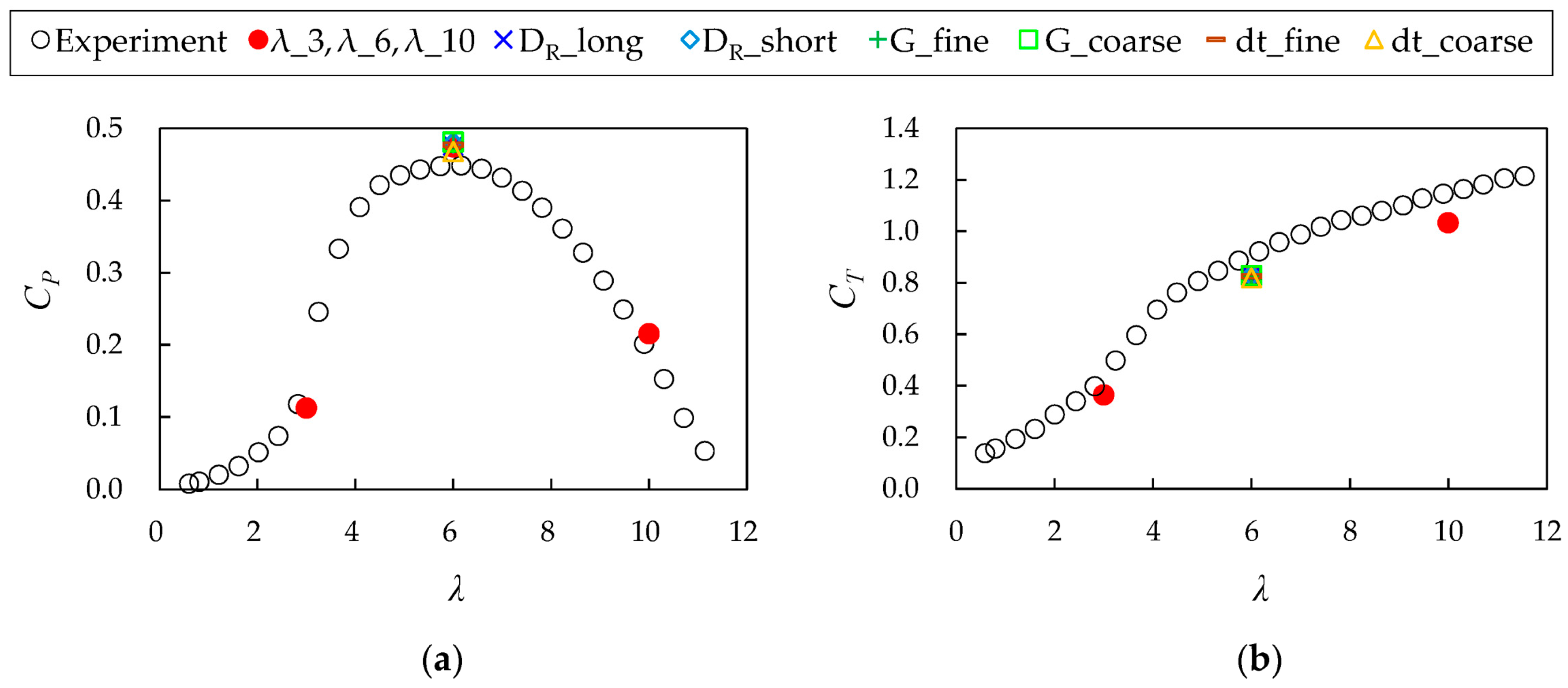
3.1. Validation of Numerical Approach

Figure 3 compares the values of the power coefficient C_P (=2QΩ/ρAU_ref³) and the thrust coefficient C_T (=2T/ρAU_ref²) evaluated from the simulations to those obtained from the wind-tunnel experiments [18]. Here, Q is the torque on the rotor, A is the rotor swept area, and T is the total thrust on the blades. The simulations provide a reasonable qualitative and quantitative approximation of the experimentally observed results for both C_P and C_T. The discrepancies of C_P and C_T between case λ_6 and other cases with λ = 6 are very small and are at most 0.0067 (dt_coarse) and 0.0048 (G_coarse), respectively.

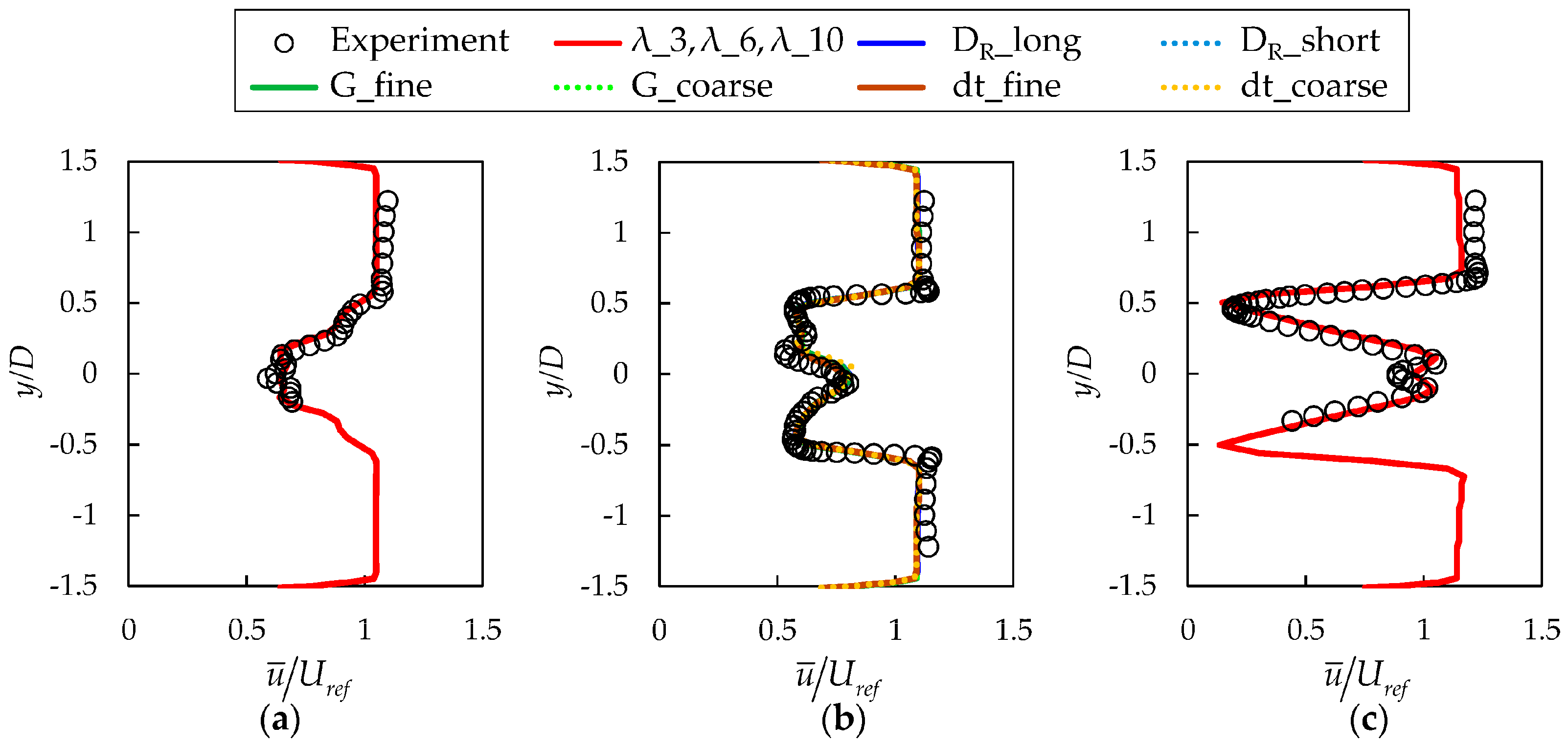
Figure 4 compares the simulation and wind-tunnel experiment results for the distribution in the y direction of $\overline{u}$ at the hub height in the wind-turbine wake at x/D = 1. The simulated values for $\overline{u}$ strongly match the experimental results [17,18] qualitatively and quantitatively. The discrepancies of $\overline{u}$ between case λ_6 and other cases with λ = 6 are very small.

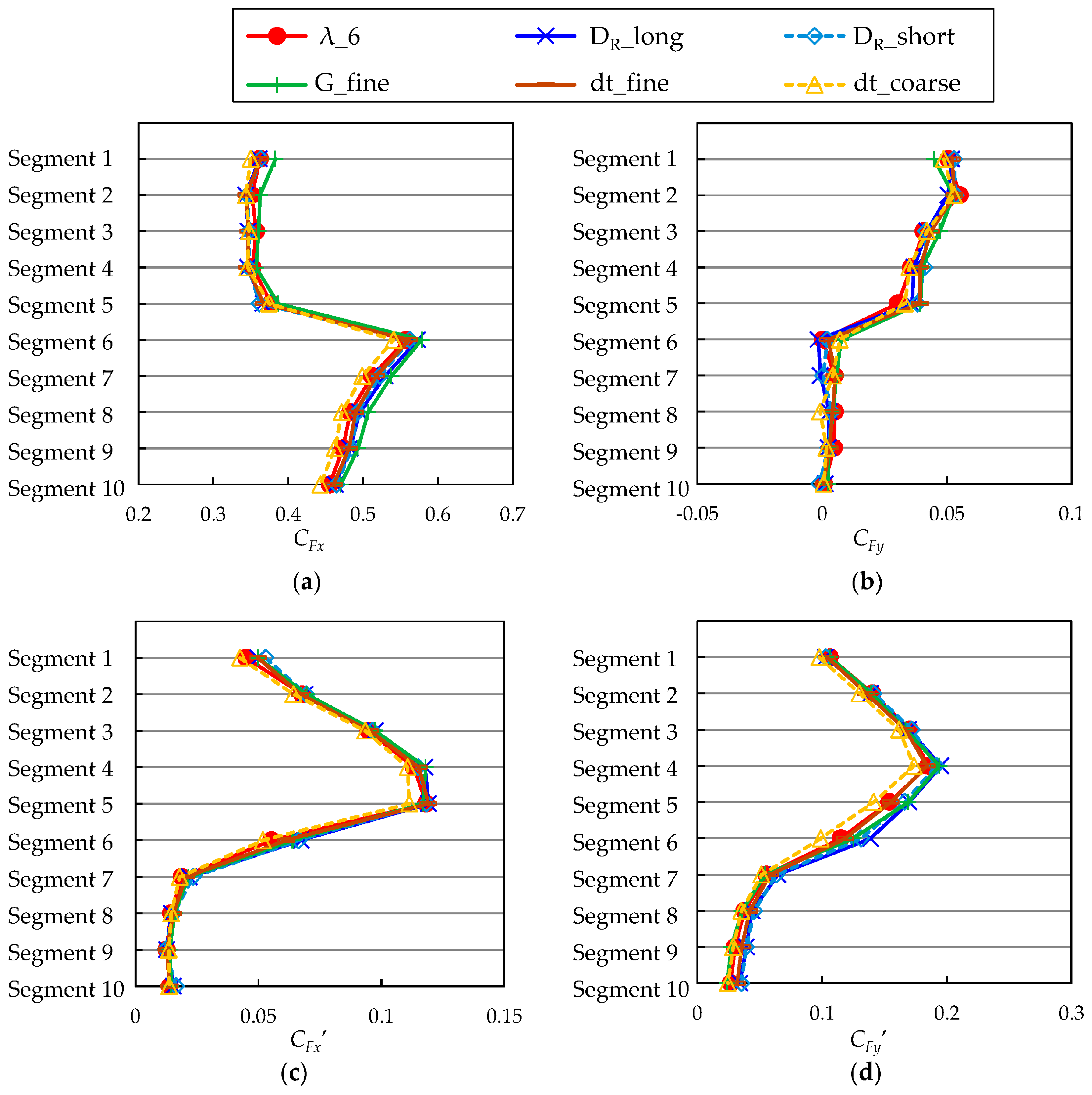
Figure 5 shows the sensitivity of D_R, the grid resolution of the structured mesh region near the tower, and dt on the vertical distributions of the mean drag coefficient C_Fx (=$2{\overline{F}}_x/{{\rho \mathit{hdU}}_{\mathit{ref}}}^2$), the mean lift coefficient C_Fy (=$2{\overline{F}}_y/{{\rho \mathit{hdU}}_{\mathit{ref}}}^2$), the fluctuating drag coefficient C_Fx’(=$2{\sigma }_{\mathit{Fx}}/{{\rho \mathit{hdU}}_{\mathit{ref}}}^2$) and the fluctuating lift coefficient C_Fy’(=$2{\sigma }_{\mathit{Fy}}/{{\rho \mathit{hdU}}_{\mathit{ref}}}^2$) of each tower segment. Here, F_x and F_y are the drag and lift forces, respectively, acting on each tower segment, and σ_Fx and σ_Fy denote the root mean squares of F_x and F_y, respectively. Except for case G_coarse, which is not shown in the figures, the discrepancies of these drag and lift coefficients between case λ_6 and other cases with λ = 6 are small.

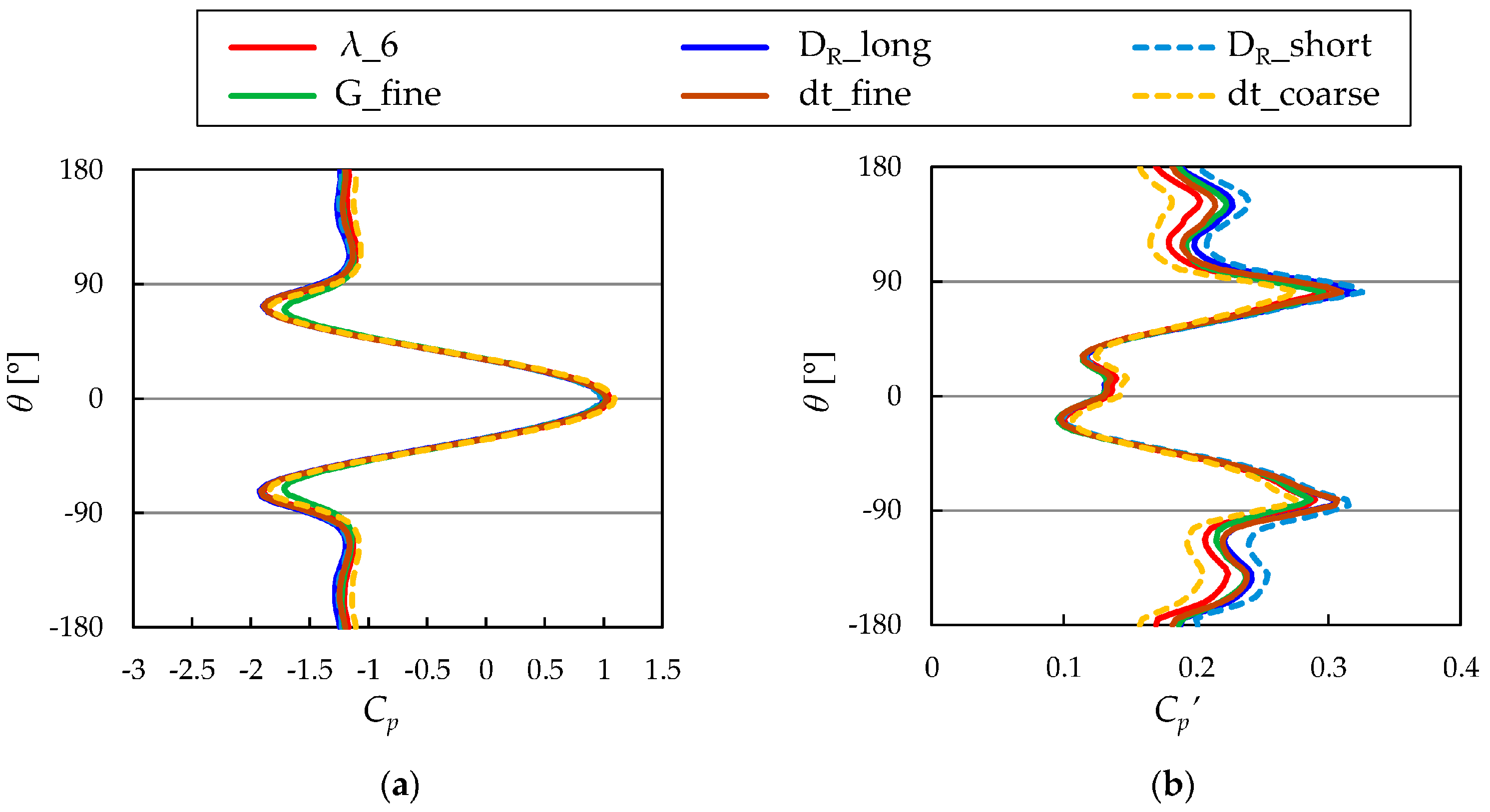
Figure 6 shows the sensitivity of D_R, the grid resolution of the structured mesh region near the tower, and dt on the horizontal distributions of the mean pressure coefficient C_p (=$2(\overline{p}-p_{\mathit{ref}})/{{\rho U}_{\mathit{ref}}}^2$) and the fluctuating pressure coefficient C_p’ (=${2\sigma }_p/{{\rho U}_{\mathit{ref}}}^2$) on the tower surface at the mid-height of Segment 6. 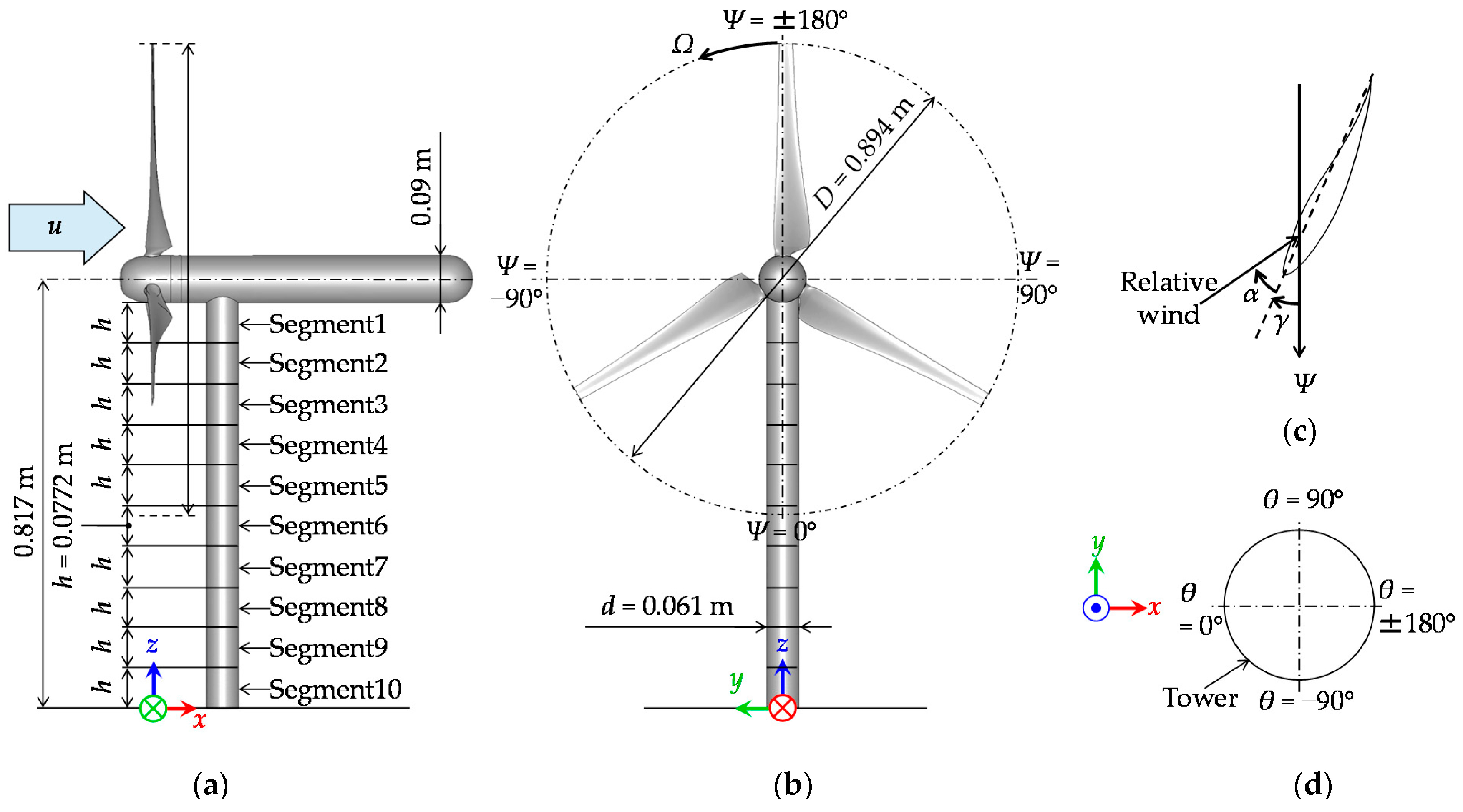Here, p_ref is the mean static pressure at (−4.1D, 0, 0.91D), σ_p denotes the root mean square of p, and θ is the azimuth angle around the tower, whose direction is defined in Figure 1d. Except for case G_coarse, which is not shown in the figures, the discrepancies of these pressure coefficients between case λ_6 and other cases with λ = 6 are small. This tendency is observed at other heights.

The aforementioned comparisons with the wind-tunnel experiments and the aforementioned sensitivity analyses indicate that the grid resolution, the rotational-domain size, and the time-step sizes for cases λ_3, λ_6, and λ_10 are reasonable for discussing the characteristics of the aerodynamic forces acting on the tower. In the following sections, the results for cases λ_3, λ_6, and λ_10 are discussed.

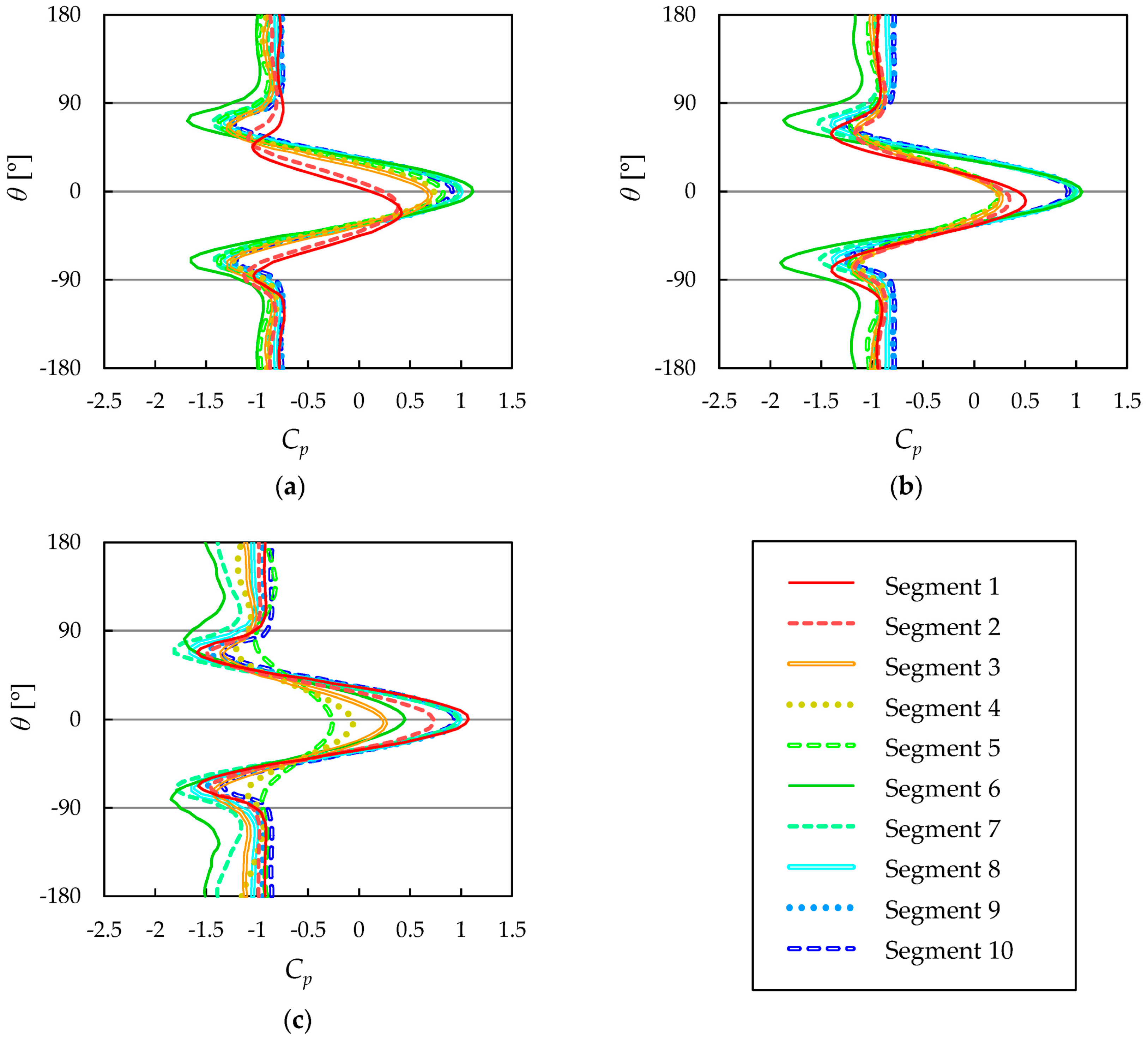
3.2. Pressure Coefficients on the Tower

Figure 7 shows the distributions of C_p on the tower surface at the mid-heights of each tower segment. When λ = 10, the distributions of C_p around the tower are almost symmetric with respect to θ = 0 for all segments. However, when λ = 3 and λ = 6, the angle θ at which C_p is maximized shifts in the −θ direction at upper segments, particularly at segments 1 and 2. This shifting is caused by the diversion of the flow approaching the tower by the rotating blades.

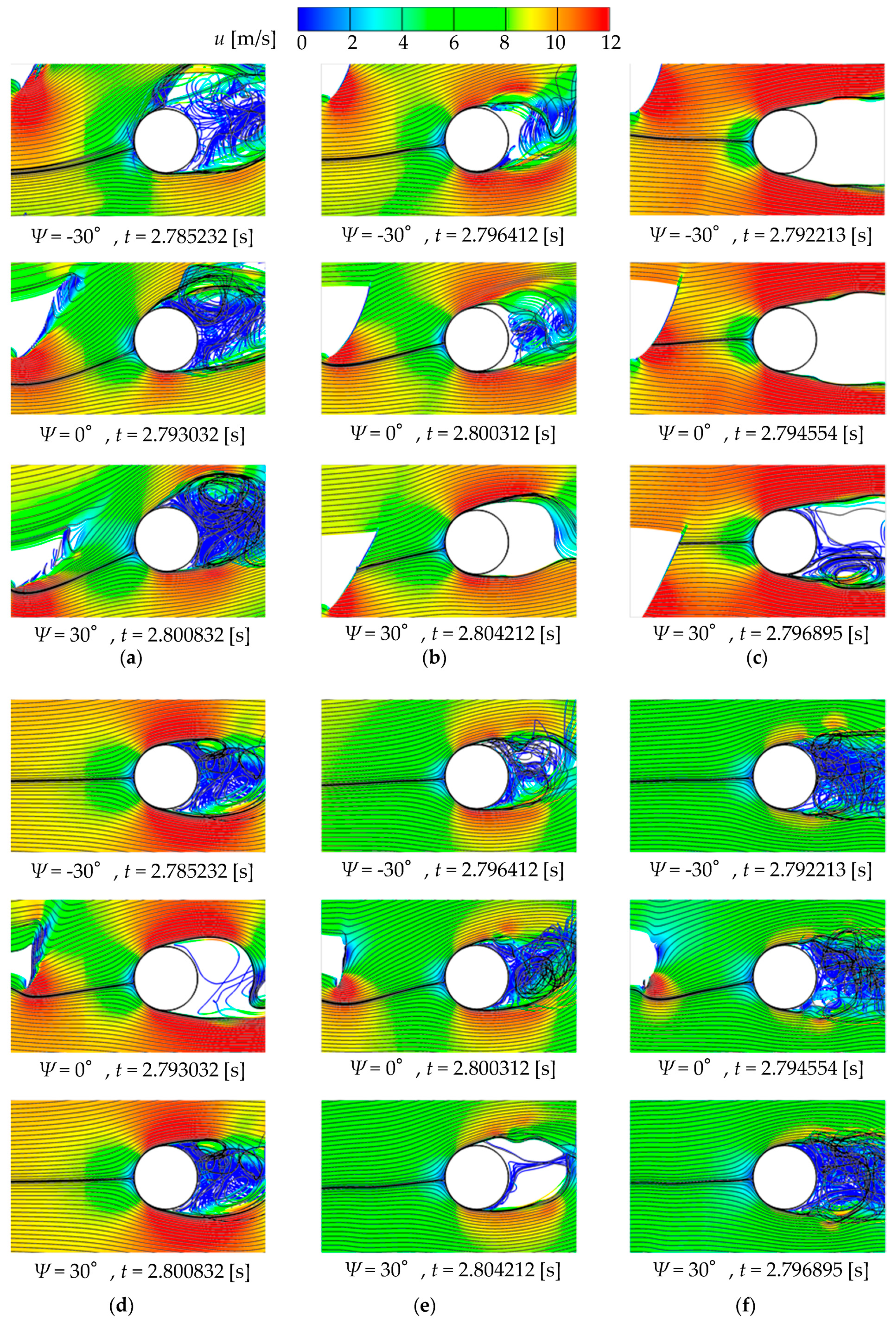
Figure 8a,b show the streamlines at the mid-height of Segment 1 for λ = 3 and λ = 6, respectively. In both figures, at all values of Ψ, the blade near the tower significantly diverts the flow approaching the tower, and the stagnation point on the tower shifts in the −θ direction. The degree of the diversion of the flow is more significant when λ = 3 than when λ = 6. Conversely, when λ = 10, the degree of the diversion of the flow due to the blade near the tower is very small at all values of Ψ, as shown in Figure 8c.

Hence, the flow diversion caused by the rotating blades becomes less significant as λ increases, which could be due to the decrease of the aerodynamic force acting on the blades in the −Ψ direction arising from the reduction of the angle of attack on the blade (α, which is defined in Figure 1c), as shown in

Table 2. Angle of attack of the blade at Ψ = 0° at the mid-height of each tower segment.

Segment of the Tower	α When λ = 3	α When λ = 6	α When λ = 10
1	28.59°	9.59°	−3.98°
2	25.28°	7.32°	−2.01°
3	21.74°	7.07°	0.33°
4	19.16°	7.16°	1.93°
5	17.75°	7.71°	3.46°

. This leads to smaller drag and lift coefficients of the blades. Previous studies [19,23] indicate that the lift coefficient of the S826 airfoil is 0 at α ≈ −5° and is maximized at α ≈ 15°. Additionally, the drag coefficient of the S826 airfoil is in the range of approximately 0.5–1.0 when −10° ≤ α ≤ 15° and increases sharply at α ≥ 15° owing to the onset of a stall. 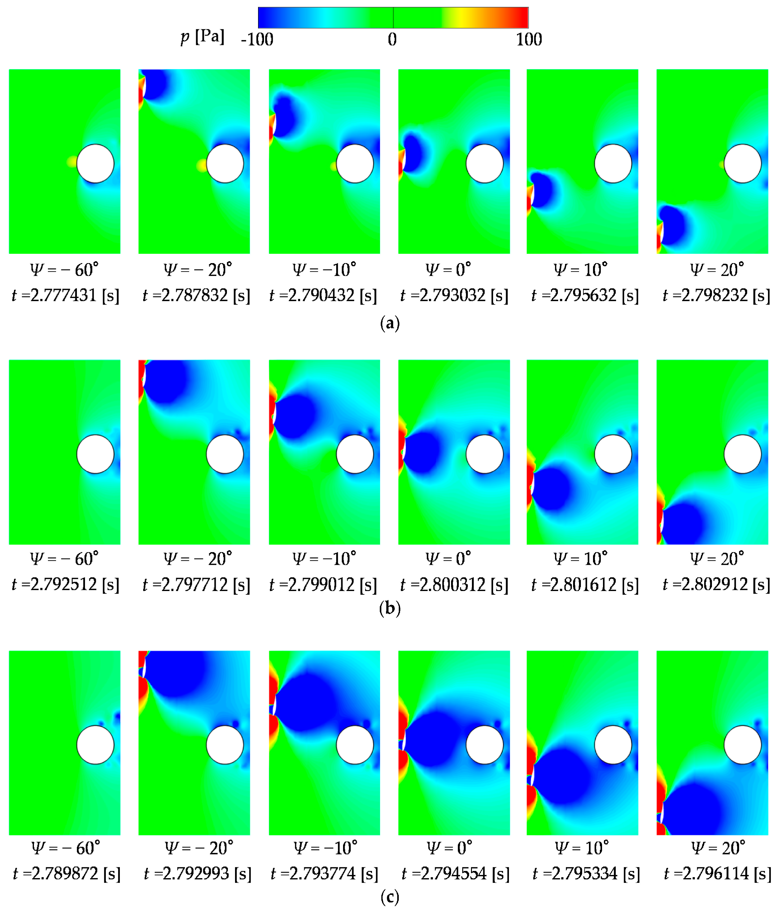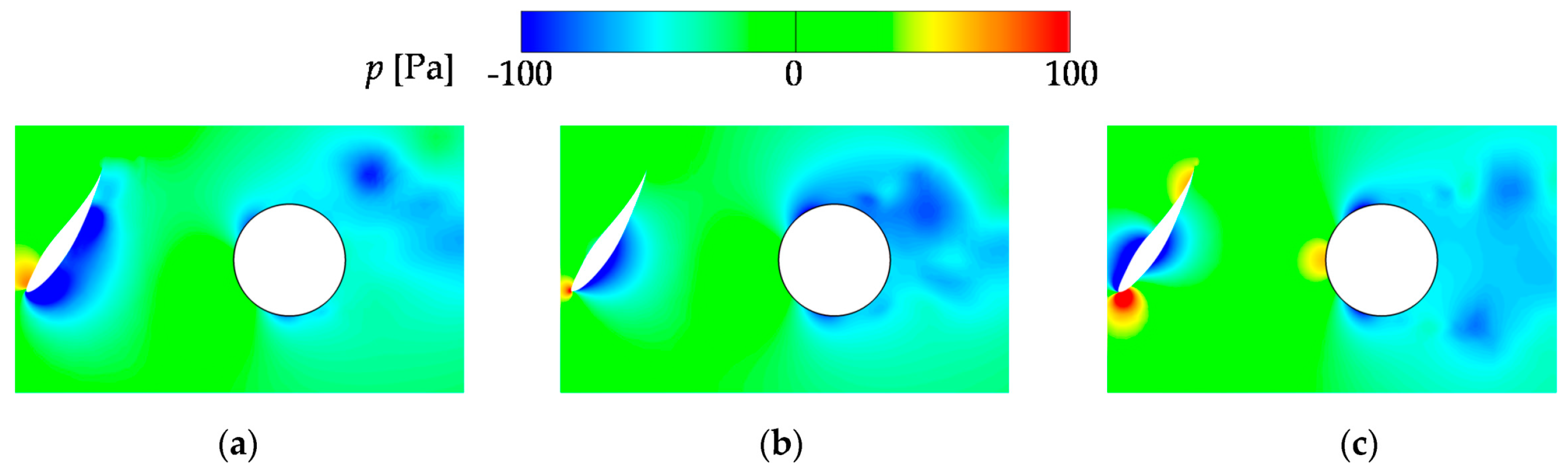The decreases in α and the aerodynamic force acting on the blades with an increase in λ leads to higher u values in the region between the rotor and tower, as shown in Figure 8a–c; higher p values on the downwind side of the blade, as shown in Figure 9; and higher maximum C_p values around the tower at the mid-height of segment 1, as shown in Figure 7.

When λ = 3, the maximum values of C_p at the mid-heights of Segments 3–5 are larger than those of Segments 1 and 2, as shown in Figure 7a. This is mainly attributed to the decrease in the drag force acting on the blades, which reduces the wind velocity. The decrease in the drag force acting on the blade with an increase in the radial distance from the rotational axis (or with a decrease in the distance from the floor when the blade is at Ψ = 0°) is mainly attributed to the decrease in α, as shown in Table 2. When λ = 6 and λ = 10, the maximum values of C_p at the mid-heights of Segments 3–5 are smaller than those of Segments 1 and 2, as shown in Figure 7b,c, respectively. This tendency is more significant when λ = 10, mainly because of the increase in the lift force acting on the blade, which reduces the wind velocity. The increase in the lift force acting on the blades with an increase in the radial distance from the rotational axis could be caused by the increase in the relative wind velocity experienced by the blade. When λ = 10, the increase in the lift force acting on the blades with an increase in the radial distance from the rotational axis could also be a result of the increase in the lift coefficient of the blade with an increase in α.

In Figure 8d–f, the flow approaching the tower is significantly diverted by the blade when Ψ = 0°. However, for all other values of Ψ, the diversion of the flow approaching the tower by the blades is very small. This explains that the amount of shifting of θ at which C_p is maximized is very small at the mid-heights of Segments 3–5 for all the λ values shown in Figure 7.

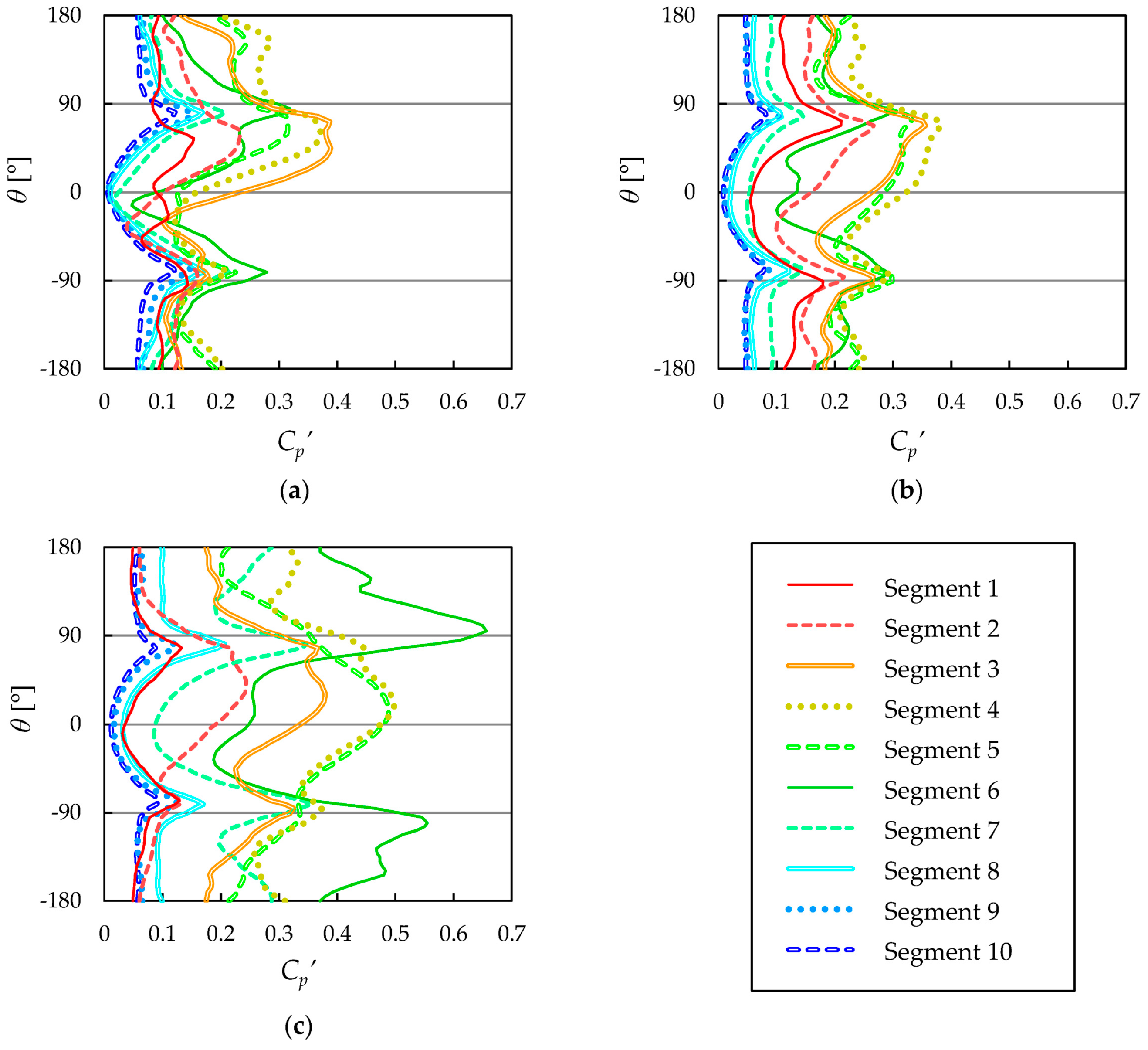
Figure 10 shows the distributions of C_p’ on the tower surface at the mid-heights of each tower segment. For all λ values, the distributions of C_p’ around the tower are almost symmetrical with respect to θ = 0 at the segments near the floor. However, with the exception of these segments, the values of C_p’ are generally higher in the +θ region than in the −θ region. This tendency could be caused by two factors when a blade passes the tower segments. The first factor is the low pressure region that forms on the downwind side of the blade. This region lowers the pressure on the tower. The second factor is the diversion of the flow approaching the tower by the blade, which shifts the stagnation point on the tower in the –θ direction.

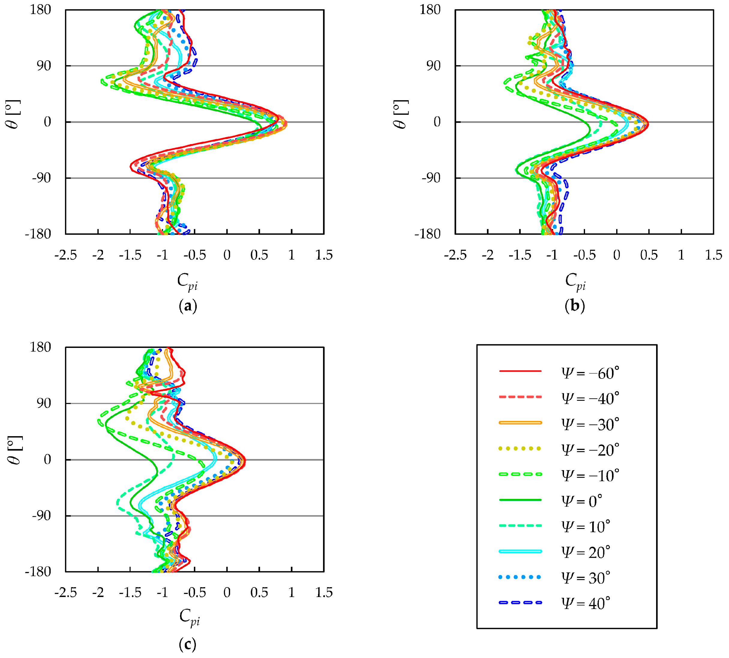
Figure 11 shows the pressure distribution at the mid-height of segment 4. As indicated by the figure, the pressure near the tower is reduced for all λ values as the blade approaches the tower. The pressure recovers when the blade moves away from the tower. Figure 12 shows the distributions of the instantaneous pressure coefficient C_pi (=$2(p-p_{\mathit{ref}})/{{\rho U}_{\mathit{ref}}}^2$) on the tower surface at the mid-heights of segment 4 when the blade nearest the tower is at various Ψ values. As shown in this figure, the θ at which C_pi is maximized on the upwind side of the tower generally shifts in the –θ direction when the blade is near the tower (such as when Ψ = –20° to 20°) for all λ values. This shift in θ at which C_pi is maximized is due to the shifting of the stagnation point on the tower.

When the blade approaches the tower, the values of C_pi on the +θ side are generally lower than those on the −θ-side. This is because the distance from the lower-pressure region on the downwind side of the blade is shorter on the +θ side than that on the –θ-side. Conversely, when the blade moves away from the tower, the values of C_pi on the –θ-side are generally lower than those on the +θ side. This is due to the distance from the lower-pressure region on the downwind side of the blade. However, when the blade moves away from the tower, the decrease in p on the −θ-side surface of the tower is suppressed by the shifting of θ at which C_pi is maximized in the −θ direction owing to the shifting of the stagnation point. Therefore, the degree of decrease in p on the −θ-side surface of the tower when the blade moves away from the tower is generally smaller than that on the +θ-side surface of the tower when the blade approaches the tower. As a result, the values of C_p’ are generally higher on the +θ-side surface of the tower than those on the −θ-side surface.

3.3. Drag and Lift Coefficients of the Tower

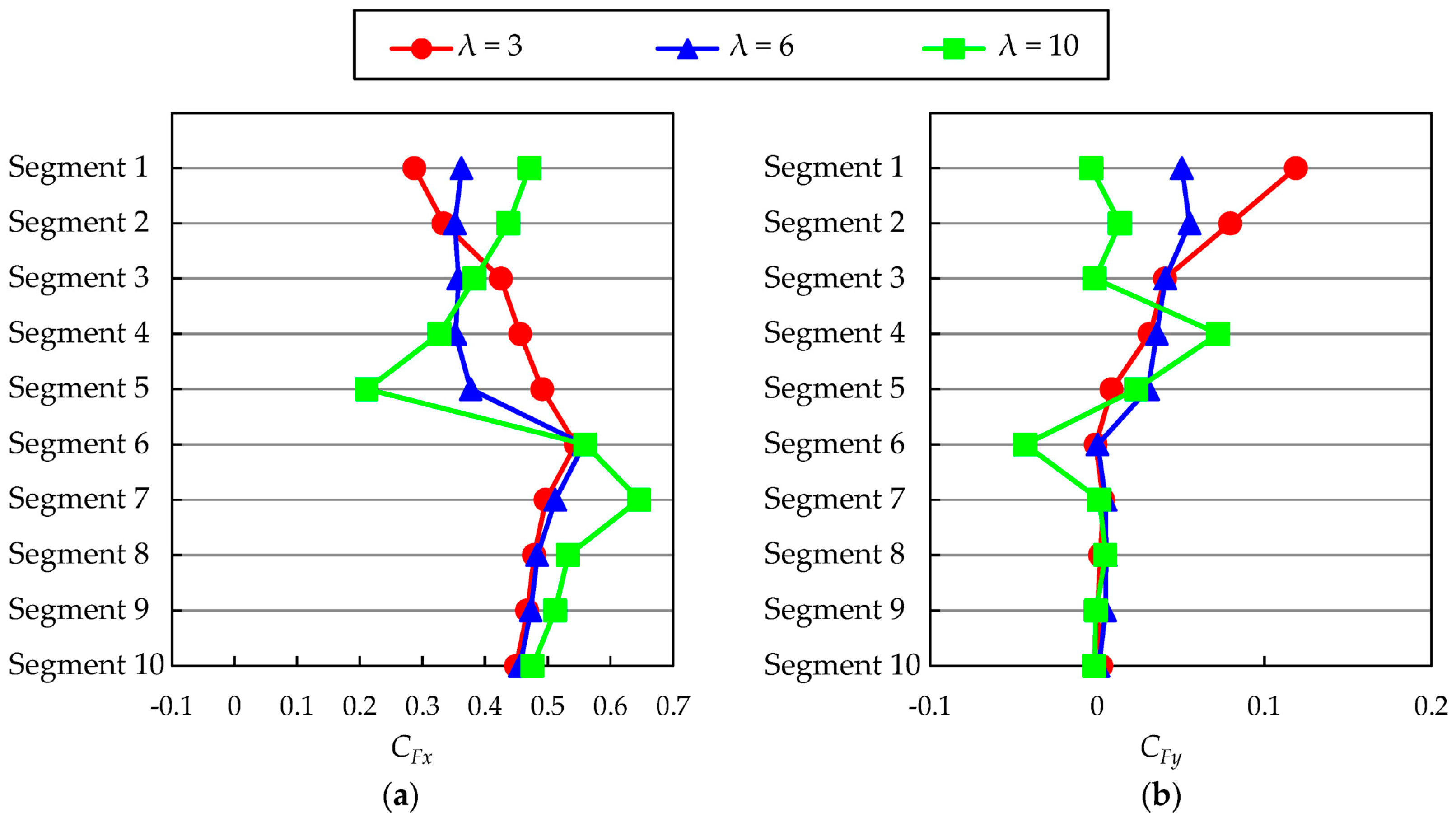
Figure 13 shows the vertical distributions of C_Fx and C_Fy of each tower segment. Figure 13a indicates that C_Fx is maximized at Segment 6 when λ = 3 and λ = 6, and at Segment 7 when λ = 10, in Figure 13a. Hence, C_Fx is the maximum at a height close to and lower than the lowest point of the rotor for all values of λ. This is because at Segment 6 or 7, the values of $\overline{p}$ are the lowest or second-lowest downwind of the tower, whereas the values of $\overline{p}$ upwind of the tower are approximately equal to those at the lower segments, as shown in Figure 7.

The aerodynamic force acting on the upper segments of the tower could be very important from the perspective of the overturning moment of the tower. In Figure 13a, the values of C_Fx at Segments 1 and 2 increase as λ increases. This is because the values of $\overline{p}$ upwind of the tower increase as λ increases as shown in Figure 7. The values of C_Fy shown in Figure 13b are very small compared with those of C_Fx. In Figure 13b, the values of C_Fy at Segments 1 and 2 increase as λ decreases. This is mainly because the values of $\overline{p}$ on the –θ-side increase owing to the increased shift in the stagnation point in the −θ direction as λ decreases, as shown in Figure 7.

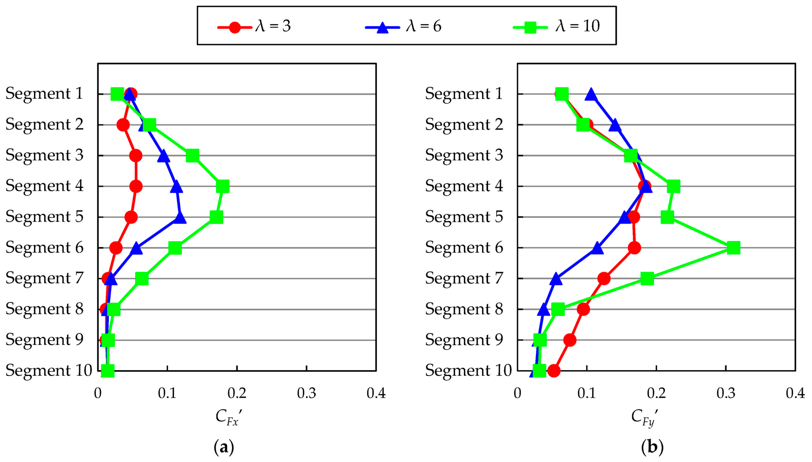
Figure 14 shows the vertical distributions of C_Fx’ and C_Fy’ of each tower segment. Here, the values of C_Fx’ are smaller than those of C_Fy’ at all segments for all values of λ. Figure 14a shows that for all values of λ, the values of C_Fx’ at Segments 1–5, which are higher than the lowest point of the rotor, are larger than the values of C_Fx’ at the segments near the floor.

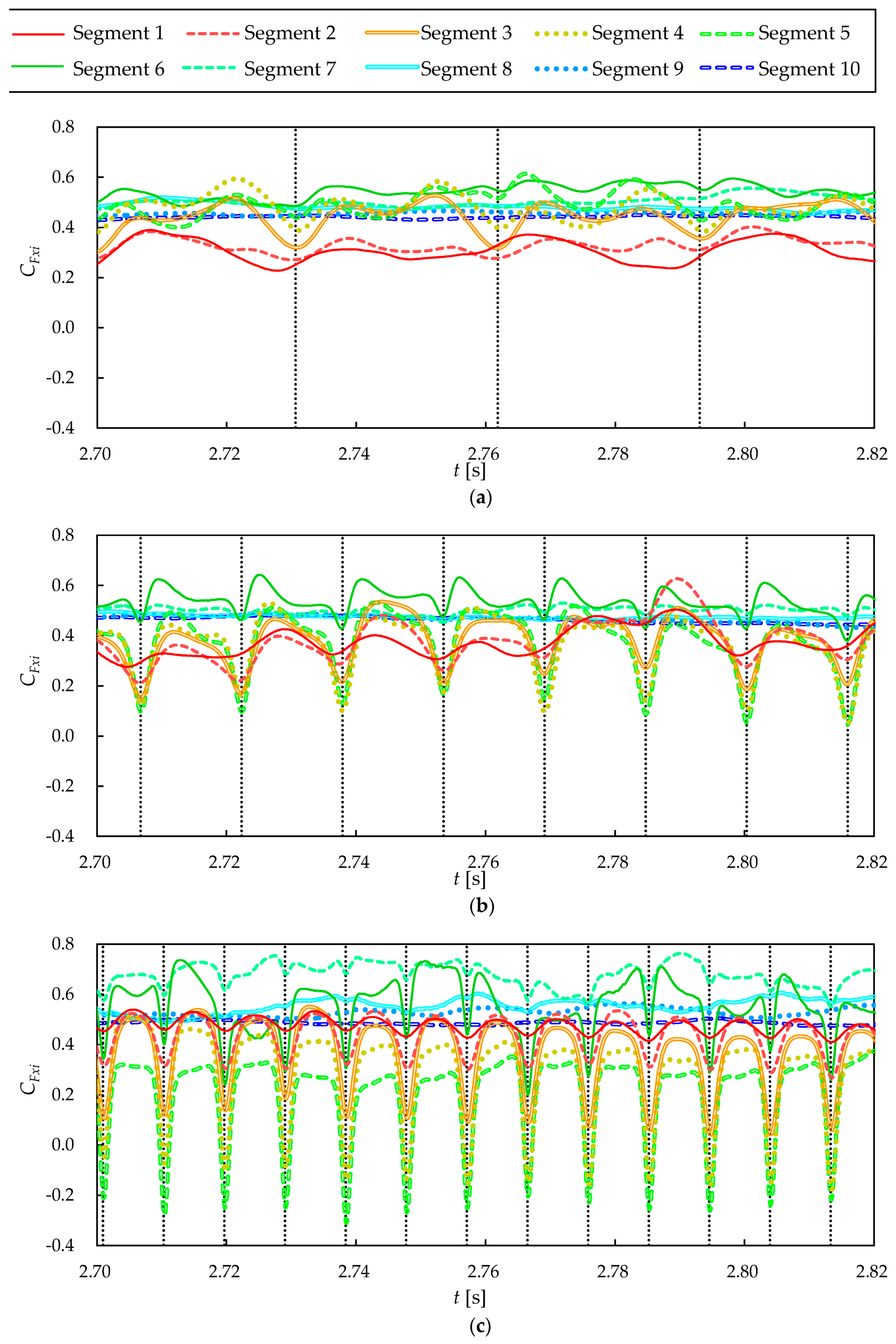
Additionally, the values of C_Fx’ are particularly large at Segments 3–5 and are maximized at one of these segments for all values of λ. The large fluctuations in F_x at these segments are caused by the decrease and subsequent increase in F_x that occur when a blade approaches and then moves away from the tower, as shown in Figure 15. This figure shows the time-history curves for the instantaneous drag coefficient C_Fxi (=$2F_x/{{\rho \mathit{hdU}}_{\mathit{ref}}}^2$) of each tower segment.

The decrease and subsequent increase in F_x at Segments 3–5 that occur when a blade approaches and then moves away from the tower are mainly due to the decrease in the values of p upwind of the tower segments caused by the lower-pressure region formed downwind of the blade, as discussed in the previous section. With an increase in λ, the magnitude of the decrease in F_x increases, as shown in Figure 15, and the maximum values of C_Fx’ at Segments 3–5 increase, as shown in Figure 14a, because the values of p downwind of the blade decrease. The value of C_Fx’ at Segment 1 in Figure 14a for λ = 10 is smaller than that for λ = 3 and λ = 6. This is because when λ = 10, the decrease in p downwind of the blade that passes the tower is very small owing to the small α. The values of C_Fx’ at λ = 3 and λ = 6 are approximately equal. However, the fluctuations in p are larger upwind of the tower when λ = 3 and downwind of the tower when λ = 6, as shown in Figure 10.

Figure 14b shows that like C_Fx’, the values of C_Fy’ at Segments 1–5 are larger than the values of C_Fy’ at the segments near the floor for all values of λ. When λ = 3 and λ = 6, the values of C_Fy’ are maximized at Segment 4. When λ = 10, the value of C_Fy’ at segment 4 is the second-largest. At Segment 6, which is lower than the lowest point of the rotor, the value of C_Fy’ is maximized. The values of C_Fy’ are relatively large at Segments 3–5 for all values of λ because when a blade approaches the tower, F_y increases and then decreases, and when the blade moves away from the tower, F_y decreases further and then increases, as shown in Figure 16. 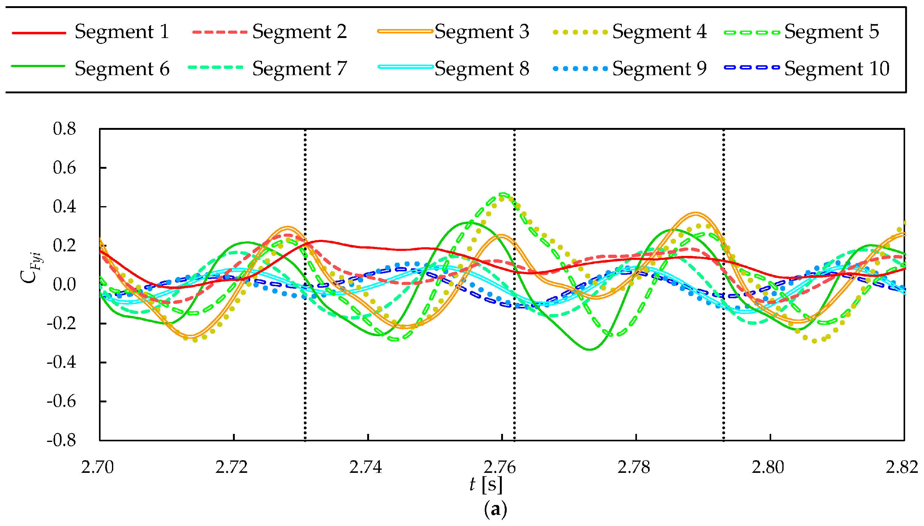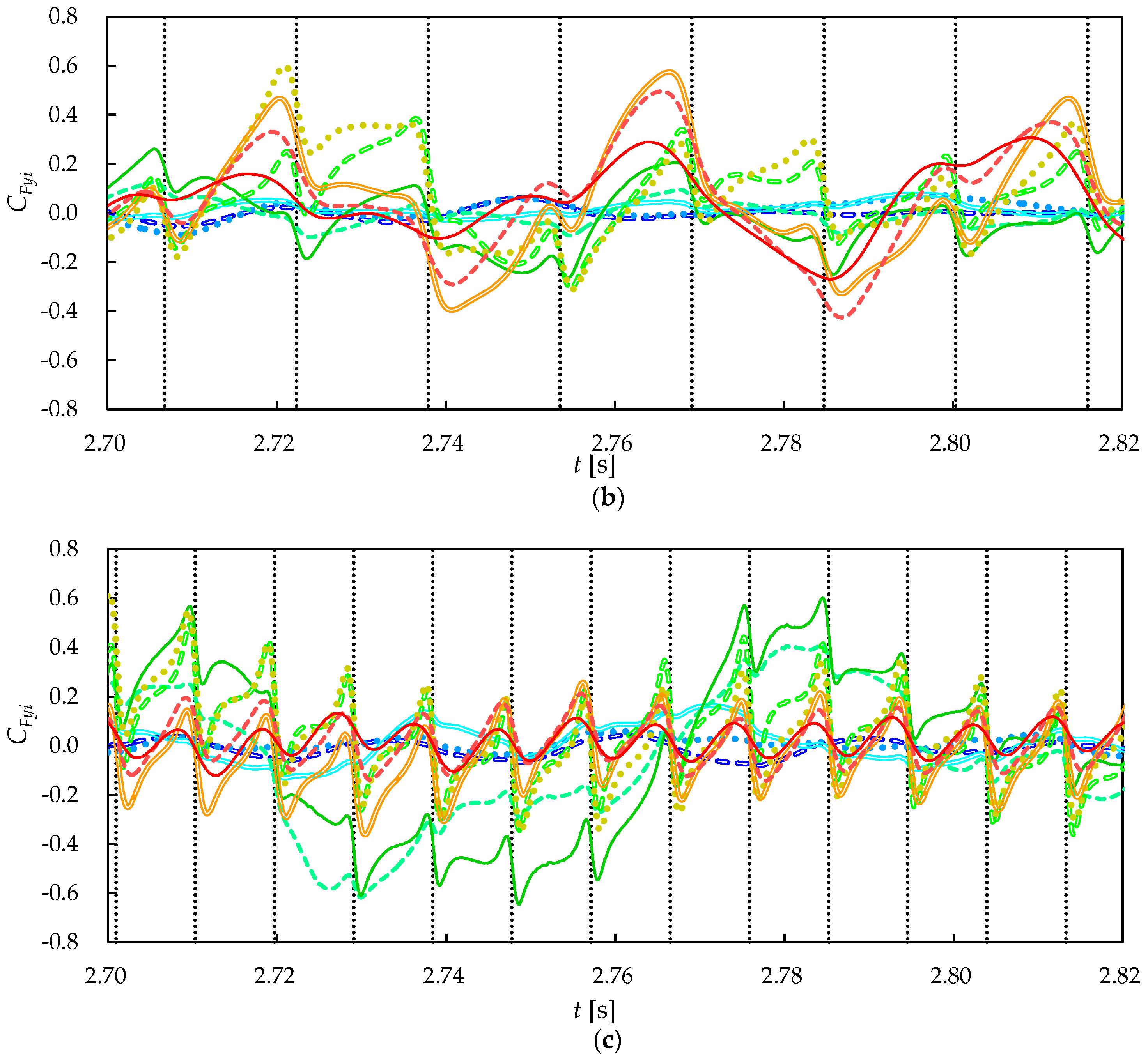Figure 16 shows the time history of the instantaneous lift coefficient C_Fyi (=$2F_y/{{\rho \mathit{hdU}}_{\mathit{ref}}}^2$) of each tower segment. Periodic fluctuation in F_y occurs because the low-pressure region downwind of the blade has a greater effect on the pressure on the +θ-side surface of the tower segments when the blade approaches the tower and a greater effect on the pressure on the −θ-side surface of the tower segments when the blade moves away from the tower, as shown in Figure 11.

C_Fy’ is maximized at Segment 6 when λ = 10 because in addition to the aforementioned fluctuation in F_y that occurs when a blade passes the tower, the F_y values fluctuate with the largest amplitude and smaller frequency than the blade-passing frequency, as shown in Figure 16. In this figure, F_y is negative at t ≈ 2.72–2.77 s and positive at t ≈ 2.77–2.81 s, with a large amplitude. This is because a strong vortex tends to form on one lateral side of segment 6 for longer periods than the blade-passing interval, followed by a similar formation on the other lateral side. Figure 14b shows that at segment 1, C_Fy’ is larger for λ = 6 than the values obtained when λ = 3 and λ = 10. This is because the value of p on the tower segment in the vicinity of θ = ± 90° fluctuates more when λ = 6, as shown in Figure 10.

4. Conclusions

As a first step toward clarifying the effects of aerodynamic forces acting on the tower of a wind turbine on the vibratory characteristics of the tower, we investigated the effects of the rotating blades of an upwind-type three-blade HAWT on the basic characteristics of the aerodynamic forces acting on its tower. This was done by conducting improved delayed detached-eddy simulations of the wind flow around the tower and the wind turbine operating at tip-speed ratios of λ = 3 (low), λ = 6 (optimum), and λ = 10 (high). The tower was divided into 10 equal segments, and the aerodynamic forces acting on each segment were analyzed.

We discovered that both the diversion of the flow approaching the tower by the rotating blades and the low-pressure region that forms downwind of the blades have significant effects on the aerodynamic forces acting on the tower. For example, owing to the diversion of the flow by the blades, the azimuth angle around the tower at which the pressure reaches a maximum at each height can shift significantly in the direction of the movement of the blade passing the tower. In addition, because of the low-pressure region downwind of the blades, the fluctuation in the lift force of the tower can be significantly larger than that in its drag force.

These characteristics of the aerodynamic forces acting on the tower might contribute significantly to the occurrence of unacceptably large stresses and deflections in the side-to-side direction when the blade passing frequency coincides with the natural frequency of the tower. Owing to the negligible contribution of the aerodynamic damping of HAWTs in the side-to-side direction, the damping ratio for the side-to-side oscillations of the tower is generally one order of magnitude less than that for the fore-aft oscillations of the tower [2]. Therefore, in future research, we plan to investigate the effects of the aerodynamic forces acting on the tower that are influenced by the rotating blades on the vibratory characteristics of the tower in the side-to-side direction by conducting fluid-structure interaction simulations. We also plan to further investigate the effects of the rotating blades of the HAWT on the basic characteristics of the aerodynamic forces acting on the tower by varying the diameter of the tower, the distance between the rotor and the tower, etc.

References

1. Manwell, J.F.; Mcgowan, J.G.; Rogers, A.L. Wind Energy Explained Theory, Design and Application, 2nd ed.; WILEY, John Wiely & Sons Ltd.: Chichester, UK, 2009; p. 379. [Google Scholar]
2. Burton, T.; Jenkins, N.; Sharpe, D.; Bossanyi, E. Wind Energy Handbook, 2nd ed.; WILEY, John Wiely & Sons Ltd.: Chichester, UK, 2011; pp. 303–305. [Google Scholar]
3. Licari, J.; Ekanayake, J.B.; Jenkins, N. Investigation of a speed exclusion zone to prevent tower resonance in variable-speed wind turbines. IEEE Trans. Sustain. Energy 2013, 4, 977–984. [Google Scholar] [CrossRef]
4. Chattot, J.-J. Extension of a helicoidal vortex model to account for blade flexibility and tower interference. J. Sol. Energy Eng. 2006, 128, 455–460. [Google Scholar] [CrossRef]
5. Gómez-Iradi, S.; Steijl, R.; Barakos, G.N. Development and validation of a CFD technique for the aerodynamic analysis of HAWT. J. Sol. Energy Eng. 2009, 131, 031009. [Google Scholar] [CrossRef]
6. Kim, H.; Lee, S.; Lee, S. Influence of blade-tower interaction in upwind-type horizontal axis wind turbines on aerodynamics. J. Mech. Sci. Technol. 2011, 25, 1351–1360. [Google Scholar] [CrossRef]
7. Hsu, M.-C.; Bazilevs, Y. Fluid-structure interaction modeling of wind turbines: Simulating the full machine. Comput. Mech. 2012, 50, 821–833. [Google Scholar] [CrossRef]
8. Li, Y.; Paik, K.-J.; Xing, T.; Carrica, P.M. Dynamic overset CFD simulations of wind turbine aerodynamics. Renew. Energy 2012, 37, 285–298. [Google Scholar] [CrossRef]
9. Wang, Q.; Zhou, H.; Wan, D. Numerical simulation of wind turbine blade-tower interaction. J. Mar. Sci. Appl. 2012, 11, 321–327. [Google Scholar] [CrossRef]
10. Hsu, M.-C.; Akkerman, I.; Bazilevs, Y. Finite element simulation of wind turbine aerodynamics: Validation study using NREL Phase VI experiment. Wind Energy 2014, 17, 461–481. [Google Scholar] [CrossRef]
11. Quallen, S.M. Development and Verification of a CFD Based Simulation Software for Floating Offshore. Ph.D. Thesis, University of Idaho, Moscow, ID, USA, 2015. [Google Scholar]
12. Duque, E.P.N.; van Dam, C.P.; Hughes, S.C. Navier-Stokes simulations of the NREL combined experiment Phase II rotor. In Proceedings of the 37th AIAA Aerospace Sciences Meeting and Exhibit, Reno, NV, USA, 11–14 January 1999; pp. 143–153.
13. Zahle, F.; Sørensen, N.N.; Johansen, J. Wind turbine rotor-tower interaction using an incompressible overset grid method. Wind Energy 2009, 12, 594–619. [Google Scholar] [CrossRef]
14. Shur, M.L.; Spalart, P.R.; Strelets, M.K.; Travin, A.K. A hybrid RANS-LES approach with delayed-DES and wall-modelled LES capabilities. Int. J. Heat Fluid Flow 2008, 29, 1638–1649. [Google Scholar] [CrossRef]
15. ANSYS, Inc. ANSYS Fluent Theory Guide, Release 17.1; ANSYS, Inc.: Canonsburg, PA, USA, 2016. [Google Scholar]
16. ANSYS, Inc. ANSYS Fluent User Guide, Release 17.1; ANSYS, Inc.: Canonsburg, PA, USA, 2016. [Google Scholar]
17. Eriksen, P.A.; Krogstad, P.Å. Experimental results for the NOWITECH/NORCOWE blindtest. Energy Procedia 2012, 24, 378–384. [Google Scholar] [CrossRef]
18. Krogstad, P.Å.; Eriksen, P.A. “Blind test” calculations of the performance and wake development for a model wind turbine. Renew. Energy 2013, 50, 325–333. [Google Scholar] [CrossRef]
19. Somers, D.M. The S825 and S826 Airfoils; Subcontractor Report NREL/SP-500-36344; National Renewable Energy Laboratory: Golden, CO, USA, 2005.
20. Spalart, P.R.; Jou, W.H.; Strelets, M.; Allmaras, S.R. Comments on the feasibility of LES for wings, and on a hybrid RANS/LES approach. In Proceedings of the First AFOSR International Conference on DNS/LES, Ruston, LA, USA, 4–8 August 1997.
21. Wilcox, D.C. Turbulence Modeling for CFD, 2nd ed.; DCW Industries, Inc.: La Canada, CA, USA, 1998; pp. 185–201. [Google Scholar]
22. Menter, F.R. Two-equation eddy-viscosity turbulence models for engineering applications. AIAA J. 1994, 32, 1598–1605. [Google Scholar] [CrossRef]
23. Krogstad, P.Å.; Lund, J.A. An experimental and numerical study of the performance of a model turbine. Wind Energy 2012, 15, 443–457. [Google Scholar] [CrossRef]
24. Luo, D.; Yan, C.; Liu, H.; Zhao, R. Comparative assessment of PANS and DES for simulation of flow past a circular cylinder. J. Wind Eng. Ind. Aerodyn. 2014, 134, 65–77. [Google Scholar] [CrossRef]
Figure 1. Geometry of the wind turbine and tower and the definitions of the angles Ψ, α, γ, and θ. (a) Side view of the wind turbine and tower; (b) front view of the wind turbine and tower; (c) cross-sectional view of the blade at Ψ = 0°; and (d) horizontal cross-sectional view of the tower.
Energies 10 00121 g001
Figure 2. Computational grid and boundary conditions. (a) Entire computational domain; (b) rotational domain; and (c) horizontal cross-section of the grid near the tower at the mid-height of Segment 3.
Energies 10 00121 g002
Figure 3. Computational and experimental results for the wind-turbine performance. (a) Power coefficient; and (b) thrust coefficient.
Energies 10 00121 g003
Figure 4. Lateral distribution of the streamwise wind velocity at the hub height in the wind-turbine wake at x/D = 1. (a) λ = 3; (b) λ = 6; and (c) λ = 10.
Energies 10 00121 g004
Figure 5. Sensitivity of DR, the grid resolution near tower, and dt on vertical distributions of the mean and fluctuating drag and lift coefficients of each tower segment at λ = 6. (a) Mean drag coefficient; (b) mean lift coefficient; (c) fluctuating drag coefficient; and (d) fluctuating lift coefficient.
Energies 10 00121 g005
Figure 6. Sensitivity of DR, the grid resolution around the tower, and dt on distributions of the mean and fluctuating pressure coefficients on the tower surface at the mid-height of Segment 6 at λ = 6. (a) Mean pressure coefficient; and (b) fluctuating pressure coefficient.
Energies 10 00121 g006
Figure 7. Distributions of the mean pressure coefficient on the tower surface at the mid-heights of each tower segment. (a) λ = 3; (b) λ = 6; and (c) λ = 10.
Energies 10 00121 g007
Figure 8. Instantaneous streamlines passing the line parallel to the y axis and tangential to the tower on its upwind side at the mid-heights of Segments 1 and 4. The circle indicates the cross-section of the tower. (a) λ = 3, Segment 1; (b) λ = 6, Segment 1; (c) λ = 10, Segment 1; (d) λ = 3, Segment 4; (e) λ = 6, Segment 4; and (f) λ = 10, Segment 4.
Energies 10 00121 g008
Figure 9. Horizontal distributions of the static pressure at the mid-height of segment 1 when the blade is located at Ψ = 0°. (a) λ = 3, t = 2.793032 (s); (b) λ = 6, t = 2.800312 (s); and (c) λ = 10, t = 2.794554 (s).
Energies 10 00121 g009
Figure 10. Distributions of the fluctuating pressure coefficient on the tower surface at the mid-heights of each tower segment. (a) λ = 3; (b) λ = 6; and (c) λ = 10.
Energies 10 00121 g010
Figure 11. Horizontal distributions of the instantaneous static pressure at the mid-height of Segment 4. (a) λ = 3; (b) λ = 6; and (c) λ = 10.
Energies 10 00121 g011
Figure 12. Distributions of the instantaneous pressure coefficient on the tower surface at the mid-height of Segment 4 for moments when the blade nearest the tower is at various Ψ values. (a) λ = 3; (b) λ = 6; and (c) λ = 10.
Energies 10 00121 g012
Figure 13. Vertical distributions of the mean drag and mean lift coefficients of each tower segment. (a) Mean drag coefficient; and (b) mean lift coefficient.
Energies 10 00121 g013
Figure 14. Vertical distributions of the fluctuating drag and fluctuating lift coefficients of each tower segment. (a) Fluctuating drag coefficient; and (b) fluctuating lift coefficient.
Energies 10 00121 g014
Figure 15. Time history of the instantaneous drag coefficient of each tower segment. The vertical dotted lines indicate the time at which the blade nearest the tower is at Ψ = 0°. (a) λ = 3; (b) λ = 6; and (c) λ = 10.
Energies 10 00121 g015
Figure 16. Time history of the instantaneous lift coefficient of each tower segment. The vertical dotted lines indicate the time at which the blade nearest the tower is at Ψ = 0°. (a) λ = 3; (b) λ = 6; and (c) λ = 10.
Energies 10 00121 g016aEnergies 10 00121 g016b