Selection and Quantification of Best Water Quality Indicators Using UAV-Mounted Hyperspectral Data: A Case Focusing on a Local River Network in Suzhou City, China

Abstract

Hyperspectral imaging performed by Unmanned Aerial Vehicles (UAVs) has proven its potential in environmental surveillances, especially in the field of water quality monitoring. In this study, three polynomial forms of inversion models for six water quality indicators were specified, with different numbers of spectral reflectance (1/2/3) as independent variables. Each model was designed with seven parameters, and the differential evolution algorithm was used to optimize the parameters by minimization of the mean absolute percentage error (MAPE) between the retrieval results and field observations. Hyperspectral data from a (UAV)-mounted imager and the corresponding river water quality measurements were obtained in a case area in Suzhou City, China. Both MAPE and the coefficient of certainty (R²) are used to evaluate the model performance. All the models are useable, with an MAPE range of 3–18% and an R² range of 0.65–0.94, while the retrieval accuracy is more indicator-dependent and two nitrogen-related indicators have the lowest MAPE of around 5%. Considering the MAPE during model training and verification, the two-band model structure is more robust than the single- or three-band structures. It is certain that such a data-driven approach for large-scale, continuous, and multiple-indicator monitoring with considerable accuracy could facilitate water quality management.

1. Introduction

Water quality monitoring is an important part of water resource assessment and water environment protection [1]. Current water quality detection is generally dependent on either water field sampling and subsequent laboratory analysis (offline) or in situ monitoring, usually using field instruments (online) [2]. Environmental monitoring in used to assess whether the temporal interval or spatial scale of the water quality data are dramatically cost-related [3]. Moreover, the online monitoring techniques are still limited to specific water quality variables. To obtain wide-range and high-frequency environmental data at a considerably lower expense, supporting precise water management and pollution control tasks, spectral remote sensing technology is increasingly showing important practical value [4]. Remote sensing spectral data have been used in the evaluation and monitoring of inland water quality indicators since the 1980s [5]. Gitelson et al. [6] showed that the wavelength range of 500–600 nm is suitable for monitoring suspension, and the reflectivity range of 700–900 nm is sensitive to the change of suspension concentration. Lobuglio et al. [7] used the Bayesian maximum entropy (BME) method to improve the estimation of Chl-a of water quality. Le et al. [8] discovered that the spectral reflectance at 520 nm has a good correlation with the turbidity of the Pearl River Estuary. Ali et al. [9] directly used the full spectral band of 400–900 nm to predict chlorophyll and total suspended solids concentrations in Lake Erie. Gu et al. [10] proposed an empirical method to study Chl-a and suspended sediment in water by specific band ratio and obtained a relatively good accuracy of about 0.815.

Quite a few inversion models for remote sensing data have been applied to marine and inland water environment monitoring. Nevertheless, the spectral data used in previous research are mostly from multispectral remote sensing [11]. The spectral resolution of commonly used multispectral remote sensing is about 70–400 nm, which makes it difficult to distinguish features with similar spectral characteristics. Due to the shortage of spectral resolution, it is inefficient to explore multispectral data using the relationship between two or more bands, resulting in low accuracy in retrieving water quality items. Hyperspectral imaging is a relatively new tool in the aquatic sciences to provide detailed observations on the water body [12]. The spectral resolution of hyperspectral remote sensing is 1–10 nm, with a much higher level of spectral details [13]. For the purpose of management, it is the basis to convert hyperspectral data into water quality information with the development of quantitative remote sensing technology and the deepening of remote sensing application [14]. However, it is still a tricky issue to convert those observed signals into widely applied and bio-chemical-based water quality indicators for the sake of effective environmental management [15]. Because of the large number of bands, it is difficult to process hyperspectral data and remove redundancy, which is the key to retrieving water quality data.

On the other hand, though the applications of remote sensing data in water quality monitoring are continually reported, they mainly focus on the relationship between chlorophyll concentration, suspended solids, and other water quality indicators with optical mechanism-based responses to spectral characteristics [16]. It is a far cry from meeting the demands of comprehensive regional and watershed environmental management. There are few quantitative studies on the measured spectral characteristics of other water quality items, including total nitrogen, total phosphorus, and chemical oxygen demand, which are frequently used in environmental management. Some argue that there is no clear correspondence between these water quality indicators and spectra in the physical sense [17], whereas others believe a significant statistical inversion is still worth trying, considering the cost and administrative convenience [18].

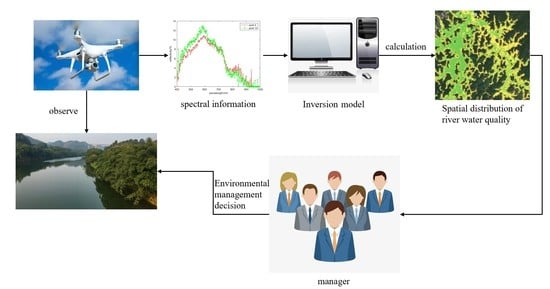
In this study, to propose a new data-driven solution for the environmental application of hyperspectral remote sensing, a hyperspectral instrument carried by an unmanned aerial vehicle (UAV) was used to obtain real-time high-resolution remote sensing image data. Using UAV as a remote sensing platform has the advantages of high timeliness and high resolution, whereas few studies have focused on the suitable relationships between multi-band hyperspectral characteristics and inland water quality [19]. Though the spatial scale of UAV-driven observation is limited, high flight frequency still ensures that abundant hyperspectral data can be obtained for the dynamic monitoring of water quality in inland lakes, reservoirs, and urban river networks [20]. Therefore, how to batch and quickly process UAV-driven hyperspectral remote sensing data becomes a bottleneck in retrieving multiple water quality indicators. In particular, there are few studies on some commonly used indicators in environmental management and environmental monitoring, such as total nitrogen, total phosphorus, permanganate index, and so on.

Therefore, this study intends to explore a feasible scheme that can convert hyperspectral data into multiple water quality indicators through optimizing both the band combination and the inversion model structure. With the case data and multiple inversion models established, it helped prove the practicability of source data from an imaging spectrometer carried by a UAV in inland water quality management. The potential application is to use hyperspectral data and relevant inversion models for routine low-cost monitoring of water quality. When increasing the flight frequency of the UAV is possible, real-time monitoring of water quality is also feasible by instantaneous processing of hyperspectral data.

2. Materials and Methods

2.1. Data Acquisition

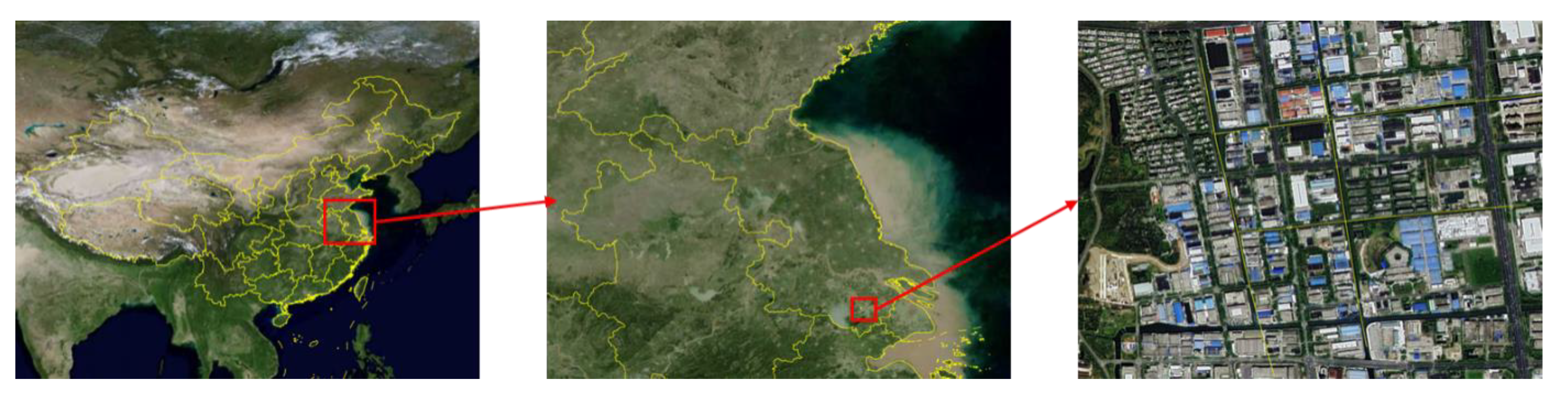
The hyperspectral data used in this study were achieved in a monitoring program carried out in a river network in Suzhou City, China. Suzhou is located in the eastern part of China, in the south-eastern part of Jiangsu Province and in the middle of the Yangtze River Delta, as shown in Figure 1. The city’s topography is low and flat, with plains accounting for 54.8% of the total area, with an altitude of around 4 meters and hills accounting for 2.7% of the total area. Suzhou has a subtropical monsoonal maritime climate with four distinct seasons and abundant rainfall.

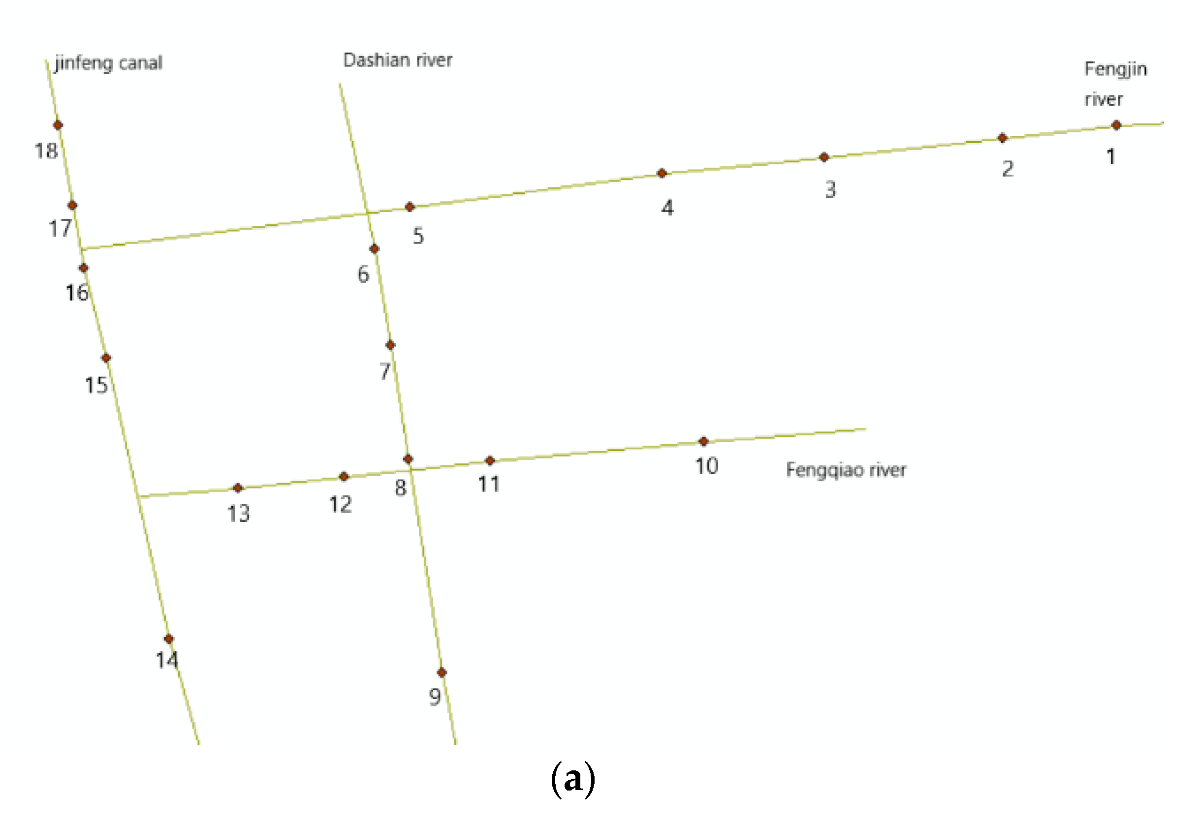
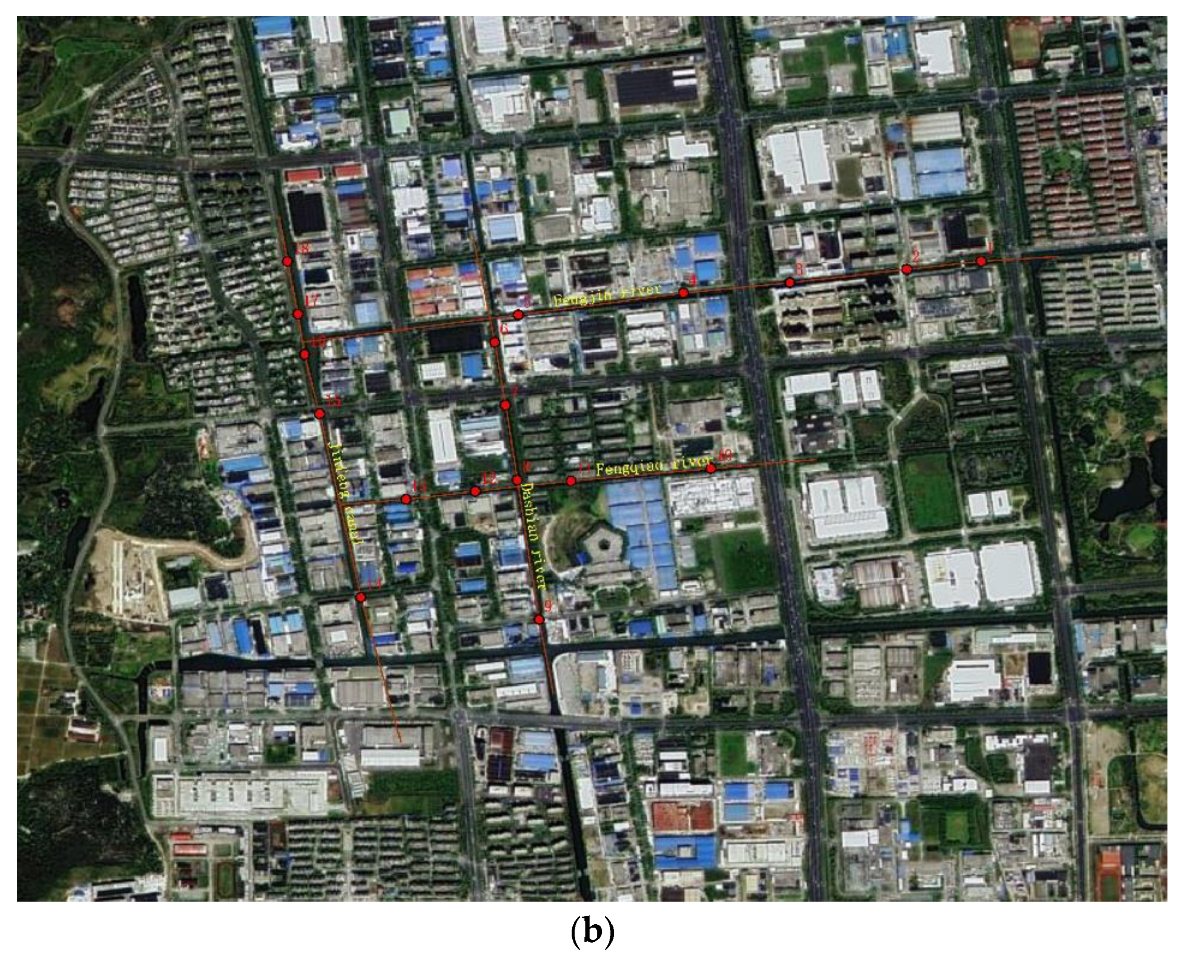
The river network is located at 120.51–120.53 east longitude and 31.30–31.31 north latitude. Four main river segments, including Fengjin river, Dashian river, Fengqiao river, and Jinfeng canal, were sampled with 5, 4, 4, and 5 sites, respectively, as shown in Figure 2. There is no routine monitoring for these river segments.

In this study, a hyperspectral imaging spectrometer was carried by a UAV for data collection. The flight altitude of the UAV was 200 m and the flight time was about 1 h. It can be regarded as single-temporal remote sensing data. In this study, the remote sensing data are from a single-temporal flight, so that atmospheric correction is not considered [21]. When the hyperspectral imaging is carried out frequently in future management, atmospheric corrections may be required in a data pre-processing step. The equipment used was a “nano-hyperspec ultra micro–Airborne Hyperspectral Imaging Spectrometer”, manufactured by American Headwall Company. The dispersion of the spectrometer is 2.2 nm, FWHM is 6 nm, and the spectral range is 400–1000 nm, with a total of 270 spectral channels and 640 spatial channels. This is an integrated hyperspectral sensor, which integrates the spectrometer, the data acquisition and storage module, and GPS/IMU inertial navigation system. This reduces the weight of the spectrometer and saves space, which allows the UAV to carry other loads such as thermal imager, lidar, and RGB camera at the same time. The UAV used in this study was the cw-15 of JOUAV, which has a maximum load of 3 kg, a cruising time of 180 min, and a flight speed of 61 km/h. After one flight, because the spectral reflectance of 953–1000 nm is 0 at more than 12 sites, spectral reflectance data of 249 spectral bands from 400 nm to 953 nm were collected.

Water sample collection in this study was carried out simultaneously with reflectance data collection. We collected three 500 mL bottles of water by boat from 0.5 m below the water surface at each of the 18 sampling sites in turn and recorded the latitude and longitude of the collection sites. At the same time, a drone collected spectral reflectance data at the same sampling sites according to latitude and longitude. As required by the water sampling standard [22], the sampling staff sank the clean sampling bottle into the water and lifted it out of the water after it was filled. Eighteen water samples were collected in this way, and they were covered with a black cloth and sent for laboratory tests of turbidity (TB, by portable turbidimeter), total phosphorus (TP, by ammonium molybdate spectrophotometry) [23], total nitrogen (TN, by alkaline potassium persulfate digestion UV spectrophotometry) [24], ammonia nitrogen (NH₃-N, by Nessler reagent spectrophotometry) [25], permanganate index (IMN, by standard method) [26], and chemical oxygen demand (COD, by rapid digestion spectrophotometry) [27], while the longitude and latitude of the sampling site were recorded. In addition, descriptive statistics for water quality data and the relative error of each test method for water quality data is also shown in Tables S1 and S2.

The water quality testing was carried out by a qualified company. The testing methods used are all current and valid environmental standards or national standard methods, and the instruments involved in the testing were all in working order. UAV spectral sampling was performed by relevant specialist engineering staff. The quality of both types of raw data can be assured.

2.2. Inversion Model Establishment

2.2.1. Define Model Structure

Because it is uncertain which model structure will be more suitable for describing the linkage between spectral features and water quality indicators, it was considered important to establish an inversion model that may represent the generalized relationship between the independent variables. Firstly, the number of independent variables in the model was chosen and classified. In this study, spectral reflectivity under one/two/three bands were selected as independent variables, respectively called single-band model, two-band model, and three-band model thereafter. Considering the structure complexity, parameter numbers were determined to be the same for three model structures.

Similar inversion studies can be implemented using machine learning methods [28], but due to the large number of parameters in machine learning algorithms and the high requirements for observed data, this study only considers the use of polynomial models for the inversion of spectral data. Although the relationship between water quality indicators and spectral data is not an ideal curve, it can be fitted with relatively high precision using the polynomial function. Due to the limited amount of data in relevant studies, the number of parameters in the polynomial model should not be too large. In this study, three polynomial models with seven parameters were established to inverse water quality indicators.

When one band is considered and the corresponding spectral reflectivity is selected as an independent variable, the model is formulated as follows:

$$y=a_1{x_1}^{b_1}+a_2{x_1}^{b_2}+a_3{x_1}^{b_3}+C$$

When two bands are considered and the corresponding spectral reflectivity are selected as the independent variables, the model is formulated as follows:

$$y=a_1{x_1}^{b_1}{x_2}^{b_2}+a_2{x_1}^{b_3}{x_2}^{b_4}+C$$

When three bands are considered and the corresponding spectral reflectivity are selected as the independent variables, the model is formulated as follows:

$$y=a_1{x_1}^{b_1}+a_2{x_2}^{b_2}+a_3{x_3}^{b_3}+C$$

where y is the concentration of specific water quality indicator, including TB, TP, TN, NH₃-N, IMN, and COD, mg/L; x₁, x₂, and x₃ are the spectral reflectivity under different bands; and a₁, a₂, a₃, b₁, b₂, b₃, b₄, and C are corresponding model parameters.

The number of parameters of the three inversion models is consistent, and they all contain 7 parameters. For single-band and three-band model structures, no product of spectral reflectivity is considered, while the two-band model structure combines both product and additive relationships. The differential evolution algorithm is used to calibrate the model parameters, and then the appropriate model structure is inferred by comparing the inversion error of multiple models.

Among the 18 groups of data, 14 groups of paired spectral and water quality data were randomly selected as the training set of the inversion model, while the other 4 groups of data were used as the verification set to validate the inversion model.

2.2.2. Select Characteristic Spectrum

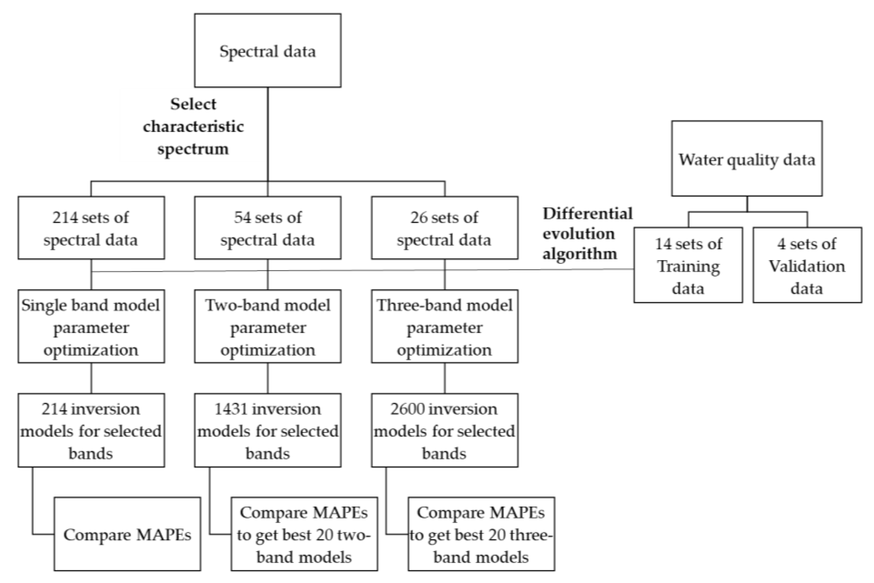
Because the hyperspectral data involve 249 different bands, the number of spectrum combinations will increase exponentially when multiple bands are selected for independent variables to retrieve water quality indicators, resulting in a high time cost of the algorithm. Therefore, it is considered important to select the representative spectra with similar spectral information in order to reduce the number of possible combinations before optimizing the parameters of the two-band and three-band inversion models.

Firstly, the band with reflectivity of 0 at multiple sampling sites is not considered for further exploration, so that the data of 249 spectral bands are reduced to 214 spectral bands. Secondly, according to the correlation coefficient between the reflectivity values of every two bands at 18 sites, spectra with corresponding correlation coefficients lower than the specific threshold were deemed as dissimilar and were then screened out for alternative independent variables. In this study, the threshold value was set as 0.7 when the two-band model was applied, while the threshold value was equal to 0.5 when the three-band model was considered. After screening, 54 bands were selected from the original 249 bands for the two-band model, while 26 bands were selected for the three-band model, named as the 54-band set and the 26-band set, respectively. All spectra either in the 54-band set or in the 26-band set were taken as characteristic spectra for alternative independent variables in the two-band model or three-band model. As a result, if only one band was considered to determine the independent variable, it was taken directly from the original 249 bands. If the number of independent variables was 2 or 3, the bands for inversion were selected from the 54-band set or the 26-band set, respectively.

2.2.3. Model Parameter Optimization and Differential Evolution Algorithm

The differential evolution algorithm was originally proposed by Storn and Price to solve the Chebyshev polynomial problem [29]. It has the advantages of less controlled parameters, strong global convergence ability, and strong robustness [30]. In recent years, differential evolution algorithms have been widely used in artificial neural networks, mechanical design, signal processing, biological information, food safety, environmental protection, and operational research [31].

The differential evolution algorithm in this study is used to adjust the parameters in the models by minimizing the mean absolute percentage error (MAPE) between the inversion results and the monitoring results of the actual water samples. The value ranges of parameters a₁, a₂, a₃, b₁, b₂, b₃, b₄, and C were defined as [−2000, 2000], [−2000, 2000], [−2000, 2000], [−2, 2], [−2, 2], [−2, 2], [−2, 2], and [−100, 100], respectively.

In this study, the differential strategy of the update variant DE/RAND/1/bin was used, which is the most widely used strategy. Moreover, the initial scale will gradually decrease with the progress of training. These settings can make the algorithm training more efficient [32]. Three most important parameters of the differential evolution algorithm are the number of individuals, the evolutionary generations, and the initial scale [33]. These three parameters will affect the time cost and the results of model training. In this study, the individual number, the evolutionary generation, and the initial scale were initially set as 100, 100, and 0.3. In order to find better settings, we respectively controlled the two parameters unchanged and adjusted the value of the remaining one, and then observed the effects on model training.

2.2.4. Screen Best Model and Technology Roadmap

The technical roadmap of this study is shown in the Figure 3.

The main purpose of this study is to establish a widely applicable data-driven water quality indicators inversion model, rather than to explore the physical relationship between a certain water quality index and the reflectance of a specific spectral band. Therefore, in the preliminary screening, only the relationship between spectral reflectance data is considered, and the physical meaning of its actual representation is not considered. When the spectral reflectance is selected as the independent variable, all choices are enumerated. The desired application scenario is that when water quality data is needed for a section of river without online monitoring equipment, the spectral data can be obtained by a drone with a hyperspectral camera, and this model can then be used to invert the required water quality data.

3. Results

3.1. Spectral and Water Quality Data Analysis

The spectral reflectance curves for the 18 sampling sites are shown in Figure S1. It can be seen that the trends in spectral reflectance data are relatively similar across the 18 sampling sites, with the main differences being in the 450–760 nm range, which is the main spectral band of interest in this study.

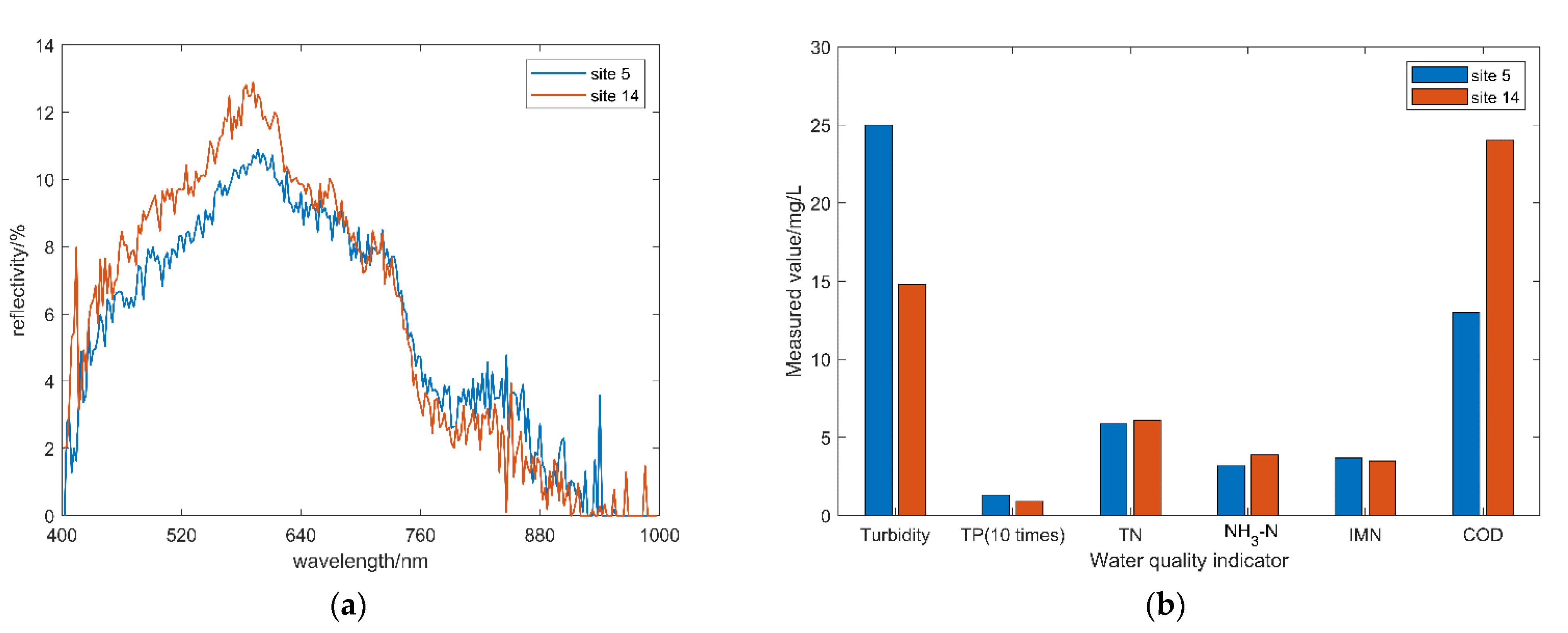
The correlation coefficients between the water quality indicators at the 18 sampling sites were calculated. It was found that the difference of water quality between site 5 (i.e., the 5th monitoring site on Fengjin river) and site 14 (i.e., the 1st monitoring site on Jinfeng canal) was the largest. Both the spectral reflectance curves and water quality indictor value of these two sites are shown in Figure 4. It can be seen that the spectral curves in the range from 430 nm and 700 nm at the two sampling sites were quite different. The reflectivity is also slightly different between 760 nm and 920 nm. There are similar situations for other sampling sites. Therefore, we can infer that, to a certain extent, the change of spectral data can reflect the difference of water quality indicators. On the other hand, the four rivers in the study area are relatively clean and the water quality gap is small, which is a great challenge for the model to screen the effective information in the spectral information.

3.2. Influence of Setting of the Optimization Algorithm

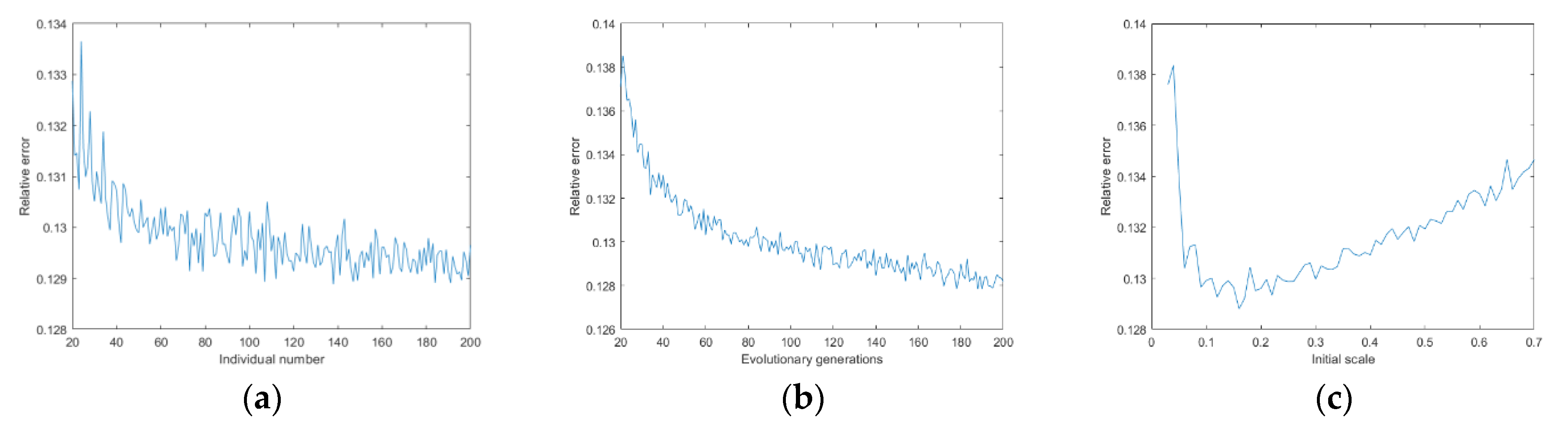
Taking the inversion of turbidity with the three-band model as an example, how the setting of the differential evolution algorithm affected the determination of inversion model parameter is illustrated in Figure 5.

It is not difficult to see from the results that with the increase of individual population, the final error decreases slightly. When the number of individual populations keep going up, the increase of error is limited. In addition, it can be seen that the more individuals there are, the less evolutionary generations needed to converge to the optimal value. However, the evolutionary generation needed for each inversion process is not very stable, unless the evolutionary generation is high enough. With the increase of the evolutionary generation, the error has a decreasing trend. With the increase of population size, the MAPE tends to be stable after 100 generations of inheritance. As for the initial scale, the results show that the smallest error is achieved when the coefficient of variation is 0.2. When the coefficient of variation is 0.1, the evolution process is quite slow and extremely unstable. When the coefficient of variation is 0.5, the convergence curve appears to have more ladder-type changes, which may be caused by easily falling into the local optimum.

Through the experiments above, better values of the algorithm settings were determined in this study, including the individual population as 100, the evolution generation as 100, and the initial scale as 0.2.

3.3. Formatting of Mathematical Components

Six water quality indicators were retrieved from 214 bands of spectral data with the single-band model. All six models with optimized parameters are shown in

Table 1. Parameter training results of single-band models.

Water Quality Indicator	Optimized Wavelength (nm)	Best Model Formula	MAPE (%)	R2
Turbidity	495	$y=-358.58x^{0.97}+24.73x^{1.6}+298.61x^{1.32}+37.69$	11.56	0.787
TP	578	$y=357.9x^{1.9}-361.87x^{1.74}+69.17x^{1.63}+0.71$	14.86	0.790
TN	629	$y=-304.42x^{1.26}-200.62x^{1.26}+214.01x^{0.78}-1.82$	4.26	0.892
NH3-N	675	$y=-148.83x^{1.71}+518.5x^{1.36}-820.54x^{1.61}+3.07$	7.01	0.879
IMN	662	$y=-325.01x^{1.29}+574.56x^{1.79}+98.13x^{1.91}+9.33$	8.43	0.840
COD	679	$y=431.59x^{1.95}-345.55x^{0.55}+342.64x^{1.09}+75.92$	17.63	0.808

, with the MAPE at 14 sampling sites, along with the coefficient of determination (R²). As for the best model formula, all exponential terms are positive. Both positive and negative values of coefficients a₁, a₂, and a₃ appear in single-band models.

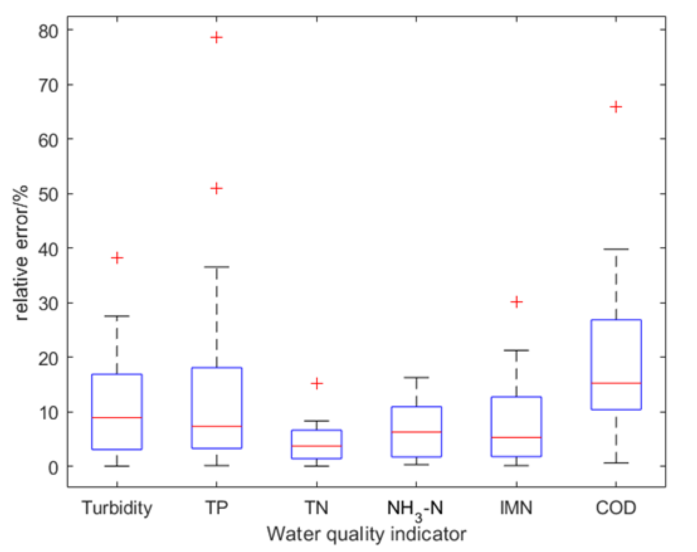
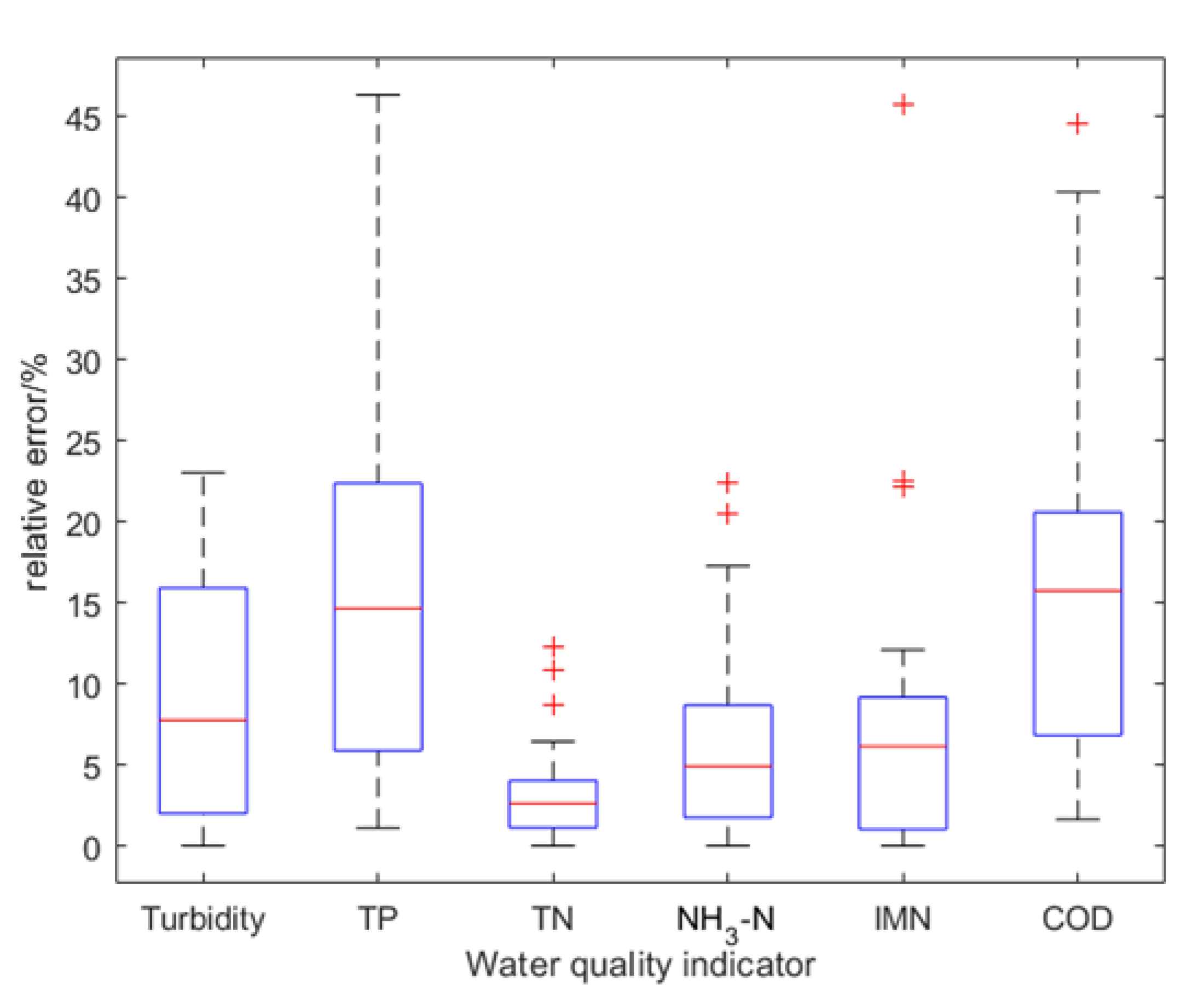
For each water quality indicator, the boxplot of relative errors at 14 sites is shown in Figure 6. It is the single-band inversion of indicator COD that has the largest MAPE, while the TP model has the largest range of relative errors.

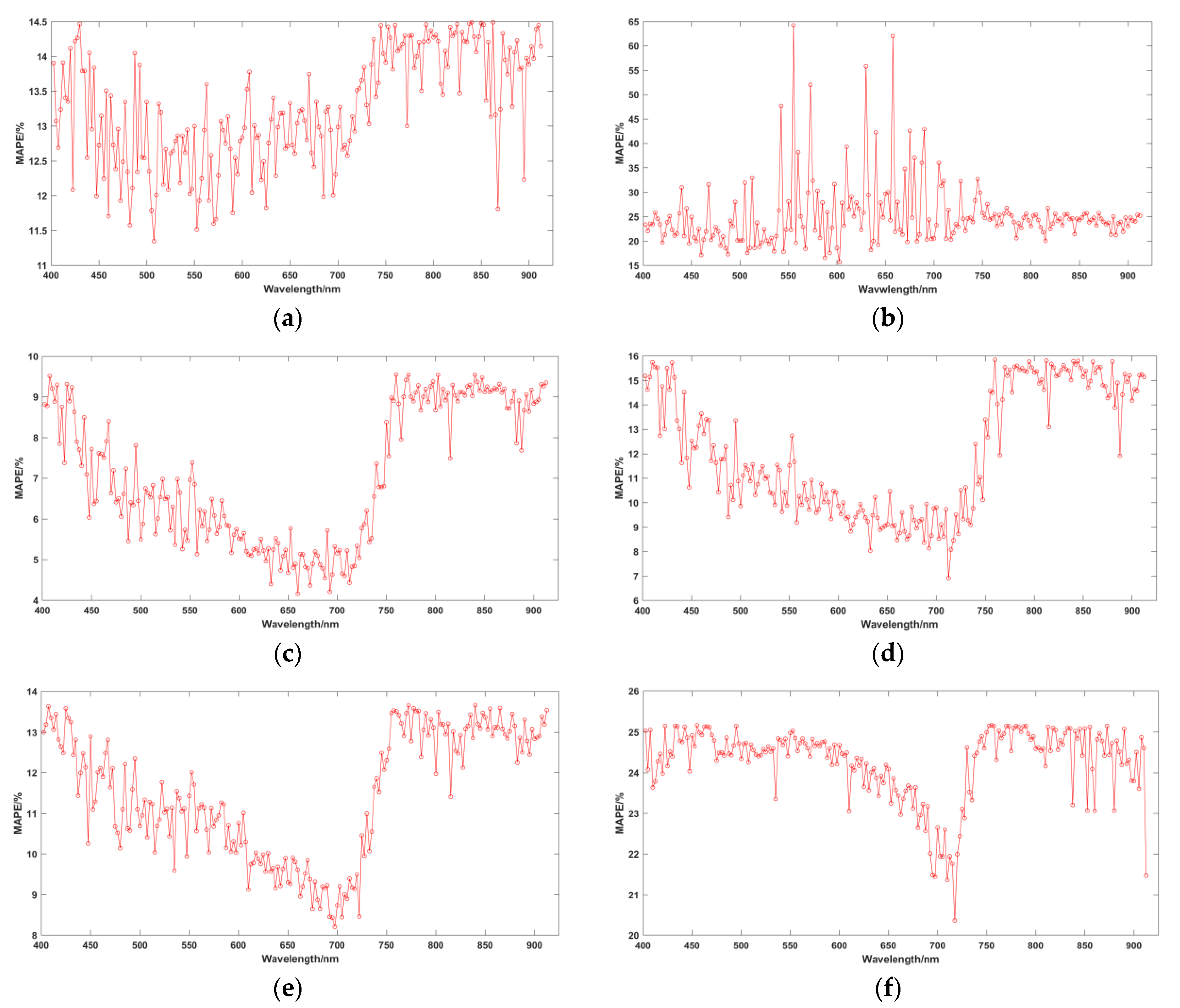
To understand the uncertainty in optimal band searching, the smallest MAPE for each band considered as the corresponding independent variable is shown in Figure 7. Though there are no similar independent variables for six inversion models, the optimized spectral bands are relatively concentrated around the wavelength of 650 nm, except for the inversion of turbidity and TP, with quite fluctuating errors under different wavelengths.

3.4. Parameter Calibration of Two-Band Models

Six water quality indicators were retrieved from optimizing the combination of 54 bands of spectral data with the two-band model structure. Among all combinations considered as the corresponding independent variables, the model with the smallest MAPE of 14 sampling sites was selected. Six two-band models with optimized parameters are shown in

Table 2. Parameter training results of two-band models.

Water Quality Indicator	Optimized Wavelength (nm)	Best Model Formula	MAPE (%)	R2
Turbidity	762, 818	$y=-824.1x_1^{0.63}{x}_2^{1.78}+69.89x_1^{-0.32}{x}_2^{1.01}+16.22$	8.62	0.823
TP	447, 718	$y=-316.99x_1^{0.62}{x}_2^{1.98}+349.63x_1^{0.57}{x}_2^{1.94}+0.23$	15.95	0.816
TN	607, 764	$y=-101.51x_1^{-0.31}{x}_2^{-0.31}+959.95x_1^{1.9}{x}_2^{-0.15}+9.57$	3.78	0.915
NH3-N	411, 607	$y=419.51x_1^{-1.48}{x}_2^{0.98}+139.42x_1^{1.04}{x}_2^{1.91}+5.39$	6.83	0.896
IMN	402, 607	$y=37.72x_1^{-1.47}{x}_2^{0.53}+234.03x_1^{1.65}{x}_2^{1.96}+5.12$	7.89	0.739
COD	722, 764	$y=-727.48x_1^{0.08}{x}_2^{0.2}-863.28x_1^{0.9}{x}_2^{1.64}+12.66$	16.60	0.800

. Some models share the same independent variables, including reflectivity under 607 nm for the inversion of TN, NH₃-N, and IMN and reflectivity under 764 nm for TN and COD model. The phenomenon that two-band models for water quality indicators TN, NH₃-N, IMN, and COD are related to mutual optimal bands with wavelength of 607 nm and 764 nm is quite similar to single-band models with optimal wavelength around 650 nm. Some explanatory mechanism needs to be discovered.

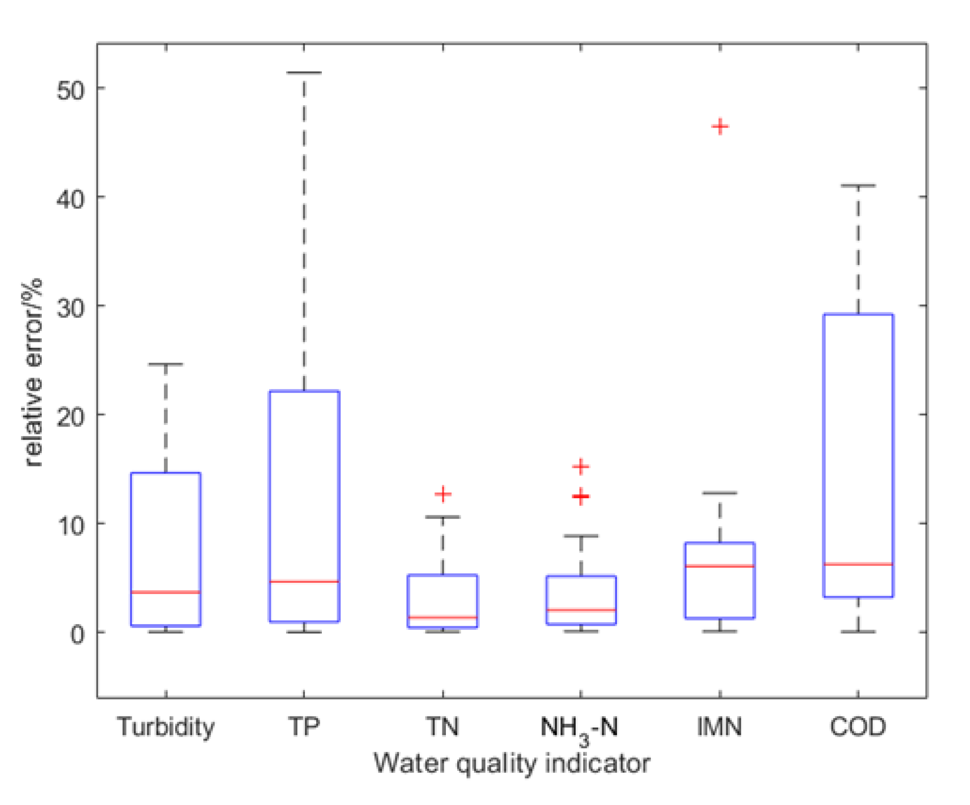
For each water quality indicator, the boxplot of relative errors at 14 sites is shown in Figure 8. It appears that both COD and TP models still have high MAPE and a wide range of errors, though the relative errors of all six two-band models slightly decrease compared with corresponding single-band models.

To investigate the uncertainty of band selection during optimization, 20 s-best inversion models with relative errors close to the optimal two-band model are chosen to explore the band characteristics. For six water quality indicators, the selected bands with the occurrence higher than 15% (i.e., three times) are shown in

Table 3. Uncertainty of band selection for two-band models.

Water Quality Indicator	Spectral Wavelength	Number of Occurrences	Water Quality Indicator	Spectral Wavelength	Number of Occurrences
Turbidity	818 nm	12	Ammonia nitrogen	607 nm	20
	422 nm	5	Permanganate index	607 nm	18
	762 nm	3	Chemical oxygen demand	764 nm	7
	813 nm	3		873 nm	4
Total phosphorus	447 nm	15		811 nm	4
	433 nm	5		409 nm	4
Total nitrogen	607 nm	20		791 nm	3

. It is reassuring that all the bands with the highest occurrences are combined in the optimal model, including 818 nm for turbidity, 447 nm for TP, 607 nm for TN, NH₃-N, and IMN, and 764 nm for COD. On the other hand, none of these bands are related to the single-band models, indicating the disadvantage of the interpretive ability of data-driven models. The inversion of indicator COD faces the largest uncertainty in terms of optimal band searching, which may partially explain the high relative errors and implies alternative inversion model structures.

3.5. Parameter Calibration of Three-Band Models

Six water quality indicators were retrieved from optimizing the combination of 26 bands of spectral data with the three-band model structure. Among all combinations considered as the corresponding independent variables, the model with the smallest MAPE of 14 sampling sites is selected. Six three-band models with optimized parameters are shown in

Table 4. Parameter training results of three-band models.

Water Quality Indicators	Optimized Wavelength (nm)	Best Model Formula	MAPE (%)	R2
Turbidity	433, 762, 818	$y=-700.35x_1^{1.86}-1015.67x_2^{1.26}+735.27x_3^{1.31}+26.01$	7.35	0.832
TP	433, 747, 838	$y=-12.14x_1^{1.76}+17.96x_2^{1.8}-41.23x_3^{1.96}+0.19$	10.04	0.652
TN	407, 676, 807	$y=206.53x_1^{1.76}-207.72x_2^{1.58}+365.64x_3^{1.84}+8.27$	3.00	0.915
NH3-N	407, 676, 822	$y=389.37x_1^{1.94}-387.38x_2^{1.95}+488.39x_3^{1.96}+4.98$	4.11	0.935
IMN	402, 433, 676	$y=-130.11x_1^{1.56}-106.42x_2^{1.57}-38.11x_3^{1.18}+7.52$	7.84	0.678
COD	429, 676, 807	$y=779.66x_1^{1.16}-345.37x_2^{0.77}+683.51x_3^{1.15}+17.96$	12.62	0.739

. All exponential terms are positive and most of them are greater than 1. It is found that the optimal wavelengths are even more concentrated in three-band models than those in single-band and two-band models. More mutual bands appear among different optimal indicator inversions, such as 407 nm, 433 nm, and 676 nm.

For each water quality indicator, the boxplot of relative errors at 14 sites is shown in Figure 9. When the relative errors of all six three-band models further decrease, compared with corresponding single-band and two-band models, the performance of the COD and TP model is still the worst.

To investigate the uncertainty of band selection during optimization, 20 s-best inversion models with relative errors close to the optimal three-band model are chosen to explore the band characteristics. For six water quality indicators, the selected bands with the occurrence higher than 15% (i.e., three times) are shown in

Table 5. Uncertainty of band selection for three-band models.

Water Quality Indicator	Spectral Wavelength (nm)	Number of Occurrences	Water Quality Indicator	Spectral Wavelength (nm)	Number of Occurrences
Turbidity	762	19	Ammonia nitrogen	676	20
	818	18		407	20
	731	3	Permanganate index	676	19
	807	3		767	12
Total phosphorus	433	18		436	4
	747	8		762	4
	873	6		402	3
	767	4		433	3
	802	4	Chemical oxygen demand	676	18
	402	3		429	12
Total nitrogen	676	20		416	5
	407	18		409	5
	436	3		816	4

. It is reassuring that all the bands with the highest occurrences are combined in the optimal model, including 762, 818 nm for turbidity, 433 nm for TP, 407, 676 nm for TN, NH₃-N, 676, 767 nm for IMN, and 429, 676 nm for COD. On the other hand, none of these bands are related to the single-band models, indicating the disadvantage of the interpretive ability of data-driven models. The inversion of indicator COD faces the largest uncertainty in terms of optimal band searching, which may partially explain the high relative errors and implies alternative inversion model structures.

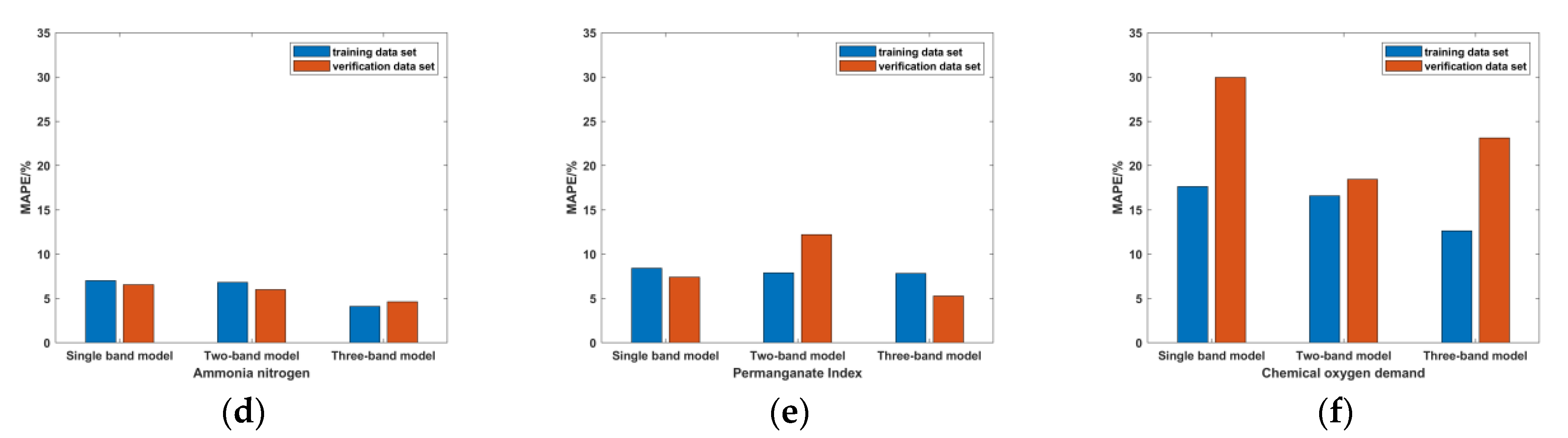
3.6. Verification of Three Types of Models

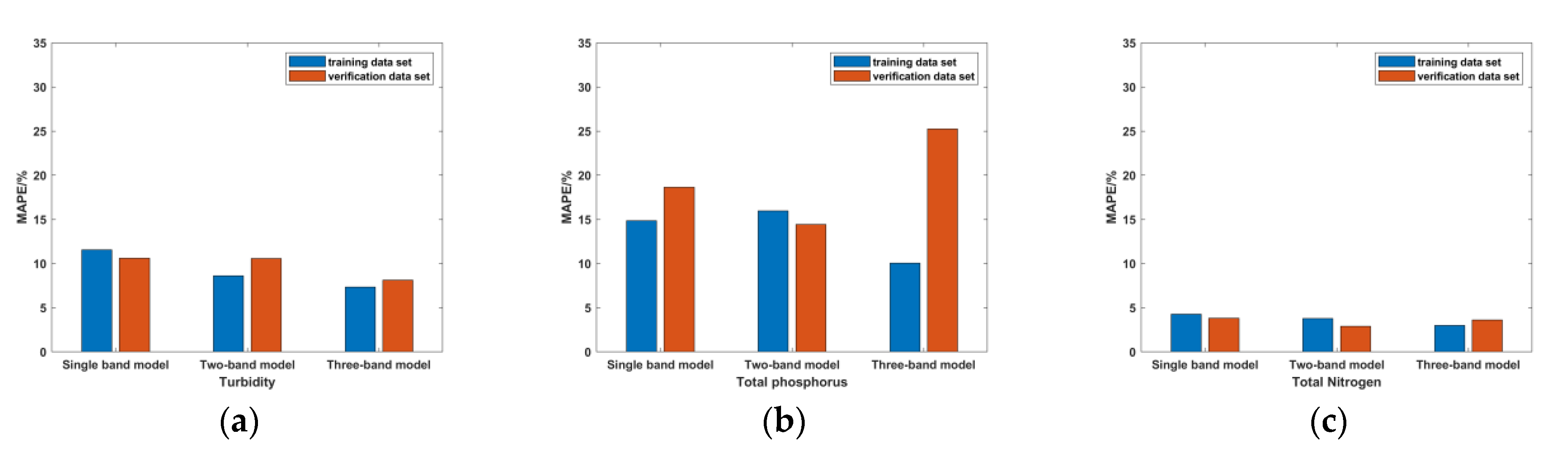
The comparison of MAPE between using 14 groups of training data and 4 groups of verification data is shown in Figure 10.

Most models have approximate training and verification errors, indicating the inversion reliability is acceptable, except for the three-band model for TP, single-band model for COD, and three-band model for COD. Considering the magnitude of relative error, the three-band models showed the best results. On the other hand, taking both training error and verification error into account, it appears that the model structure of the two-band is slightly more robust than the other two structures, in terms of water quality inversion in the case of river networks. This may be attributed to the consideration of both product and additive relationship between two bands. As for the three-band structure, though training errors were always low, highly fluctuating verification errors among different indicators implied that the prediction risk should be considered. Because limited water quality observations could be utilized in the inversion under current routine monitoring conditions, model overfitting may occur when more bands are involved.

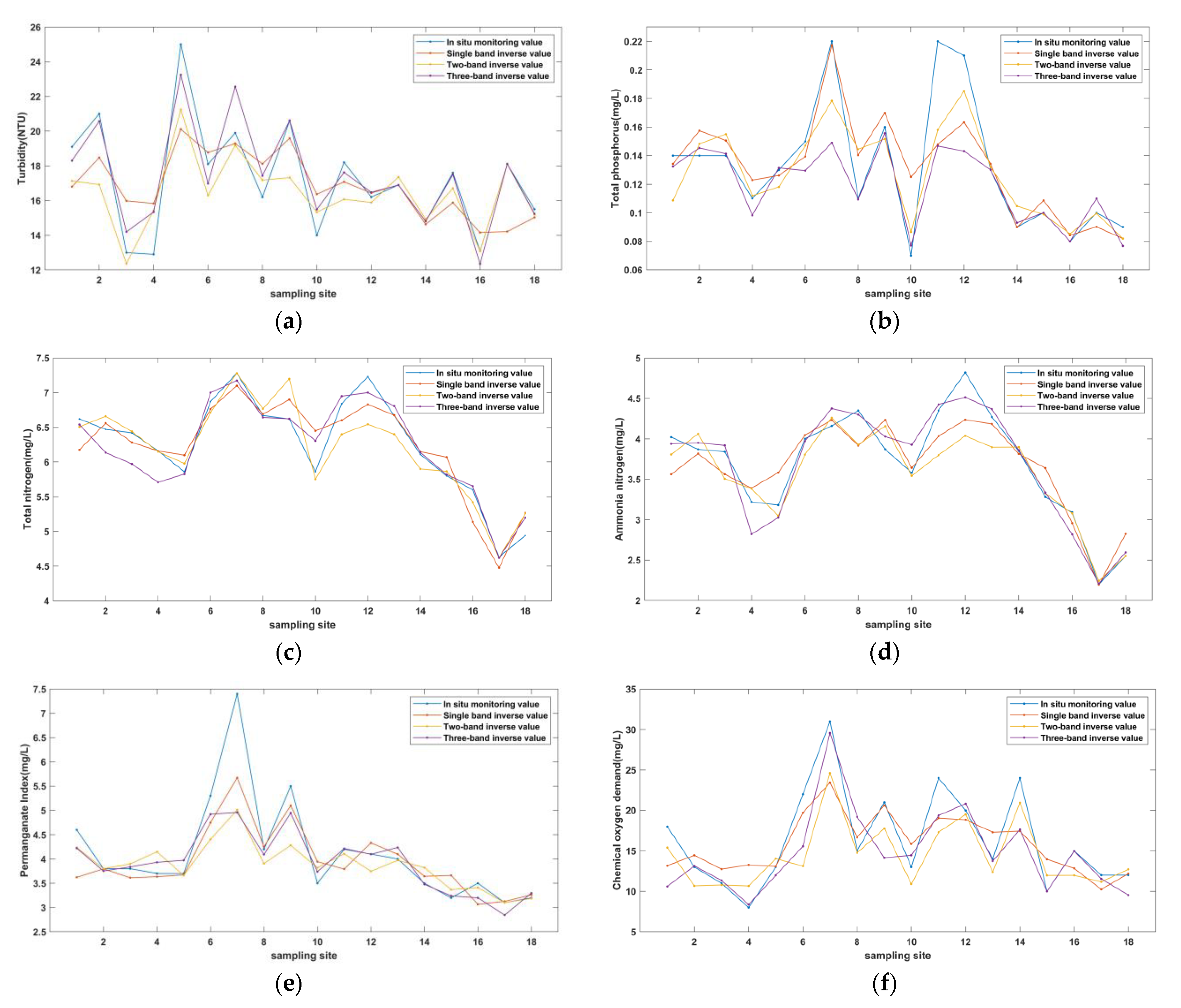
4. Discussion

The in situ measured water quality data and the inversion data for the model with the best inversion of the three structures are shown in Figure 11. It can be seen that the inversion results for all six water quality indicators are quite good. There are some differences between the inversions for different water quality indicators, with the best inversions for total nitrogen. In addition, the structure of the model with the best inversion effect for different water quality indicators is also inconsistent.

Among the 18 best model formulas, the inversion of TN and NH₃-N are most accurate, with the MAPE of TN lower than 5% and NH₃-N around 5%. As for the 6 models for TN and NH₃-N, neither over-fitting nor apparent performance differences among the three model structures is found. Moreover, in two-band and three-band model structures, inversion of TN and NH₃-N shares the same independent variables. Investigating the water quality data, the ratio of ammonia nitrogen to the total nitrogen of the case river network is quite high. Moreover, the main pollution source of the case river network is combined sewer flow, which is characterized by a high concentration of ammonia nitrogen. It is deducted that the dominant form of nitrogen in the case river segments was ammonia nitrogen. This could be one reason that inversion of TN and NH₃-N showed same independent variables and similar performance. For many urban rivers in China, water eutrophication potential is still a common challenge, in which the key influential factors are the concentration of TN and NH₃-N. Though few studies on Nitrogen-related inversion are reported, the models established in this study, which could predict the TN and NH₃-N satisfactorily, prove the high feasibility of the application of hyperspectral data from a UAV-mounted imager for supporting environmental management.

Apart from TN and NH₃-N, the performance of turbidity inversion is good enough for management purposes, with a MAPE around 10%. Compared with previous studies on turbidity and suspended solid inversion, the MAPE and R² of the inversion model in this study for turbidity are slightly better. R² was 0.76 for turbidity inversion (n = 17) [34]. Yin et al. [35] constructed a ratio model based on the reflectivity at 684 nm and 540 nm with data from the zhuhai-1 hyperspectral satellite, and inversed the suspended solids concentration in Yuqiao reservoir with the relative error of 8.6%. Overall, the characteristic bands of turbidity or suspended solids found in these studies are in the range of 480–550 nm and 680–820 nm, which is consistent with the spectral band selected by the two-band and three-band models with the best inversion accuracy in this study.

The inversion performance of permanganate index is also pretty good, with the MAPE lower than 10%. The verification error of the two-band model for permanganate index was slightly higher, indicating the possibility of over fitting. Unfortunately, few similar studies can be referenced for cross-verification of IMN inversion. COD is another popular indicator for organic pollution representation. In our study, though the COD inversion results somehow were worse than other water quality indicators, the relative error could be controlled at around 20% by selecting appropriate model structures. Because the monitoring data of COD and IMN indicated that the case river network was rather clean, it is more appropriate for such a water body to use IMN to characterize the degree of organic pollution than COD. Therefore, both the IMN and COD inversion models are acceptable from the perspective of practical management. Moreover, the inversion results of COD in previous studies are generally worse than those in this study. Bansod et al. [36] inversed COD concentration through spectral index combination regression, and R² was between 0.5 and 0.6. Peterson et al. [37] found that COD was related to the spectrum of 400 nm to 800 nm, which is quite a large range. In this study, the selected bands of the COD inversion model are also varied, but much more concentrated.

TP is another indicator whose inversion performs plainly, with a MAPE around 15%. According to the water quality data, the TP concentration of the case river network was very low and far below the quality requirement, which means the TP would not be a major concern for the case river protection. Some studies showed better results of TP inversion. For instance, the spatial distribution parameterization method of Du et al., based on an artificial neural network (ANN), predicts that phosphorus with R² exceeded 0.9, but this method does not have strong robustness to different data sets [38]. Song et al. [39] believe that there is a strong link between phosphorus concentration and 450 to 630 nm spectral reflection data, which is roughly consistent with the band selected by the single-band model in this study.

Though the improvement of the TP and COD models may not be that urgent in the case area due to its specific water quality features, further exploration for the expansion of inversion applications is still necessary. In our study, the single-band model and the three-band model do not contain the reflectance ratio relationship between bands, whose validation results of indicators TP and COD are relatively poor and indicate the inclination to over fitting. To achieve better inversion, the model structure may need to be adjusted. For example, similar to the two-band model, the relationship term of reflectivity ratio among different bands may need to be considered in the three-band model for TP and COD.

Moreover, the spectral bands are preliminarily screened when establishing the two-band and three-band models because of the computation cost. In the case where sufficient computational resource is available, we could consider to skip over the preliminary screening step and observe whether there is significant reduction of inversion error and change of independent variables in various models. Because the amount of data in this study is not large, only seven parameters were selected in various models. If more spectral and corresponding water quality data can be obtained in the future, more complex models can be used to try to uncover the information of water quality hidden in spectral data.

5. Conclusions

In this study, based on hyperspectral reflection data collected by a UAV-mounted imager, we established three groups of polynomial models with structures characterized by different combinations of hyperspectral bands, taking MAPE as the optimization goal, and used differential evolution algorithm to quantitatively predict the concentration of multiple water quality indicators, including turbidity, TP, TN, NH₃-N, IMN, and COD. The inversion performance is good enough for management purposes, with MAPE and R² similar to or better than previous research. The MAPEs of six indicators are about 7–11%, 10–16%, 3–4%, 4–7%, 7–8% and 13–17%, respectively. Considering the fitting degree of the models to the data set, the R² of models for six indicators are about 0.79–0.84, 0.65–0.82, 0.89–0.92, 0.8–0.94, 0.67–0.84 and 0.74–0.81, respectively. Meanwhile, for these six different indicators, the hyperspectral characteristic bands are 495, 762, 818 nm (turbidity); 433–447, 578 nm (TP); 407, 607–676 nm (TN and NH₃-N); 607–676, 767 nm (IMN); and 429, 676–811 nm (COD). It is concluded that this method can effectively help monitor the water quality of urban rivers in real time and provide necessary support for the decision-making of water environment protection.

This method uncovers the relationship between certain spectral reflectance and multiple pollutants in water that cannot be described by physical or chemical mechanism. The polynomial forms of multiple indicator models help manifest the advantage of the data-driven solution. Because it is easy for UAV sampling to cover more areas and conduct continuous scanning, further research may acquire more relevant spectral and water quality data, so that the method could be improved and applied in different types of water bodies. With further application, this method is practical for tracking the pollution sources of urban rivers and supporting an early warning system for efficient pollution control.

Concerning further research, it is worth exploring the phenomenon that inversion performance is more indicator-dependent and less affected by polynomial structures tested in the case of river networks. Other types of model structures containing the relationship between different continuous reflectance are encouraged in order to achieve higher robustness, especially in the three-band model. Undoubtedly, the parameters and structure of the inversion models for different water bodies may need to be readjusted. A follow-up study also needs to be carried out to reduce the complexity and time cost of the algorithm.

References

- Nazemi, A.; Wheater, H.S. How can the uncertainty in the natural inflow regime propagate into the assessment of water resource systems? Adv. Water Resour. 2014, 63, 131–142. [Google Scholar] [CrossRef]
- Parra, L.; Rocher, J.; Escrivá, J.; Lloret, J. Design and development of low cost smart turbidity sensor for water quality monitoring in fish farms. Aquac. Eng. 2018, 81, 10–18. [Google Scholar] [CrossRef]
- Wojtasiewicz, B.; Hardman-Mountford, N.J.; Antoine, D.; Dufois, F.; Slawinski, D.; Trull, T.W. Use of bio-optical profiling float data in validation of ocean colour satellite products in a remote ocean region. Remote Sens. Environ. 2018, 209, 275–290. [Google Scholar] [CrossRef]
- Sudduth, K.A.; Jang, G.S.; Lerch, R.N.; Sadler, E.J. Long-Term Agroecosystem Research in the Central Mississippi River Basin: Hyperspectral Remote Sensing of Reservoir Water Quality. J. Environ. Qual. 2015, 44, 71–83. [Google Scholar] [CrossRef] [PubMed]
- Bukata, R.P.; Jerome, J.H.; Kondratyev, K.Y.; Pozdnyakov, D.V. Optical Properties and Remote Sensing of Inland and Coastal Waters; CRC Press: Boca Raton, FL, USA, 2018. [Google Scholar]
- Gitelson, A.; Garbuzov, G.; Szilagyi, F.; Mittenzwey, K.H.; Kaiser, A. Quantitative remote sensing methods for real-time monitoring of inland waters quality. Int. J. Remote Sens. 1993, 14, 1269–1295. [Google Scholar] [CrossRef]
- Lobuglio, J.N.; Characklis, G.W.; Serre, M.L. Cost-effective water quality assessment through the integration of monitoring data and modeling results. Water Resour. Res. 2007, 43, 455–456. [Google Scholar] [CrossRef]
- Le, C.; Li, Y.; Zha, Y.; Sun, D.; Huang, C.; Lu, H. A four-band semi-analytical model for estimating chlorophyll a in highly turbid lakes: The case of Taihu Lake, China. Remote Sens. Environ. 2009, 113, 1175–1182. [Google Scholar] [CrossRef]
- Ali, K.A.; Ortiz, J.D. Multivariate approach for chlorophyll-a and suspended matter retrievals in Case II type waters using hyperspectral data. Hydrol. Sci. J. 2016, 61, 200–213. [Google Scholar] [CrossRef]
- Gu, Q.; Li, Q.; Zhou, M. Water Quality Monitoring of the Yangtze Estuary by Using GF-5 Hyperspectral Image. In Proceedings of the 2019 12th International Congress on Image and Signal Processing, BioMedical Engineering and Informatics (CISP-BMEI), Suzhou, China, 19–21 October 2019; IEEE: Piscataway, NJ, USA; pp. 1–5. [Google Scholar]
- Wojcik, K.A.; Bialik, R.J.; Osinska, M.; Figielski, M. Investigation of Sediment-Rich Glacial Meltwater Plumes Using a High-Resolution Multispectral Sensor Mounted on an Unmanned Aerial Vehicle. Water 2019, 11, 2405. [Google Scholar] [CrossRef]
- Benediktsson, J.A.; Chanussot, J.; Fauvel, M. Multiple classifier systems in remote sensing: From basics to recent developments. In Multiple Classifier Systems, Proceedings; Springer: Berlin/Heidelberg, Germany, 2007; Volume 4472, pp. 501–512. [Google Scholar]
- Wang, X.; Wang, X.X.; Zhao, J.H.; Fan, J.C.; Su, X.; Zou, D.J. Monitoring the Thermal Discharge of Hongyanhe Nuclear Power Plant with Aerial Remote Sensing Technology Using a Uav Platform. In Proceedings of the 2017 IEEE International Geoscience and Remote Sensing Symposium (IGARSS), Fort Worth, TX, USA, 23–28 July 2017; pp. 2958–2961. [Google Scholar]
- Bonansea, M.; Ledesma, M.; Rodriguez, C.; Pinotti, L. Using new remote sensing satellites for assessing water quality in a reservoir. Hydrol. Sci. J. 2019, 64, 34–44. [Google Scholar] [CrossRef]
- Wang, Q.A.; Wu, C.Q.; Li, Q.; Li, J.S. Chinese HJ-1A/B satellites and data characteristics. Sci. China-Earth Sci. 2010, 53, 51–57. [Google Scholar] [CrossRef]
- Gitelson, A.A.; Keydan, G.P.; Merzlyak, M.N. Three-band model for noninvasive estimation of chlorophyll, carotenoids, and anthocyanin contents in higher plant leaves. Geophys. Res. Lett. 2006, 33, 431–433. [Google Scholar] [CrossRef]
- Sokoletsky, L.; Gallegos, S. Towards Development of an Improved Technique for Remote Retrieval of Water Quality Components: An Approach Based on the Gordon’s Parameter Spectral Ratio; Naval Research Lab Stennis Space Center Ms Oceanography Division: Hancock County, MS, USA, 2011. [Google Scholar]
- Shi, K.; Zhang, Y.; Song, K.; Liu, M.; Qin, B. A semi-analytical approach for remote sensing of trophic state in inland waters: Bio-optical mechanism and application. Remote Sens. Environ. 2019, 232, 111349. [Google Scholar] [CrossRef]
- Gamba, M.T.; Ugazio, S.; Marucco, G.; Pini, M.; Presti, L.L. Light weight GNSS-based passive radar for remote sensing UAV applications. In Proceedings of the 2015 IEEE 1st International Forum on Research and Technologies for Society and Industry Leveraging a Better Tomorrow (RTSI), Turin, Italy, 16–18 September 2015; IEEE: Piscataway, NJ, USA; pp. 341–348. [Google Scholar]
- Zhang, C.H.; Kovacs, J.M. The application of small unmanned aerial systems for precision agriculture: A review. Precis. Agric. 2012, 13, 693–712. [Google Scholar] [CrossRef]
- Song, C.; Woodcock, C.E.; Seto, K.C.; Lenney, M.P.; Macomber, S.A. Classification and change detection using Landsat TM data: When and how to correct atmospheric effects? Remote Sens. Environ. 2001, 75, 230–244. [Google Scholar] [CrossRef]
- HJ 494-2009; Water quality-Guidance on sampling techniques. Ministry of Environmental Protection: Beijing, China, 2009.
- GB/T 11893-1989; Water quality-Determination of total phosphorus-Ammonium molybdate spectrophotometric method. Environmental Protection Agency: Beijing, China, 1989.
- HJ 636-2012; Water quality-Determination of total nitrogen-Alkaline potassium persulfate digestion UV spectrophotometric method. Ministry of Environmental Protection: Beijing, China, 2012.
- HJ 535-2009; Water quality-Determination of ammonia nitrogen-Nessler’s reagent spectrophotometry. Ministry of Environmental Protection: Beijing, China, 2009.
- GB/T 11892-1989; Water quality-Determination of permanganate index. Environmental Protection Agency: Beijing, China, 1989.
- HJ/T 399-2007; Water quality-Determination of the chemical oxygen demand-Fast digestion-spectrophotometric method. Environmental Protection Agency: Beijing, China, 2007.
- Huang, Z.Q.; Huang, W.X.; Li, S.; Ni, B.; Zhang, Y.L.; Wang, M.W.; Chen, M.L.; Zhu, F.X. Inversion Evaluation of Rare Earth Elements in Soil by Visible-Shortwave Infrared Spectroscopy. Remote Sens. 2021, 13, 4886. [Google Scholar] [CrossRef]
- Storn, R.; Price, K. Differential evolution—A simple and efficient heuristic for global optimization over continuous spaces. J. Glob. Optim. 1997, 11, 341–359. [Google Scholar] [CrossRef]
- Vesterstrom, J.; Thomsen, R. A comparative study of differential evolution, particle swarm optimization, and evolutionary algorithms on numerical benchmark problems. In Proceedings of the Cec2004: Proceedings of the 2004 Congress on Evolutionary Computation, Portland, OR, USA, 19–23 June 2004; pp. 1980–1987. [Google Scholar]
- Ching-Tzong, S.; Lee, C.S. Network Reconfiguration of Distribution Systems Using Improved Mixed-Integer Hybrid Differential Evolution. IEEE Trans. Power Deliv. 2003, 18, 1022–1027. [Google Scholar] [CrossRef]
- Ali, M.M.; Toern, A. Population set-based global optimization algorithms: Some modifications and numerical studies. Comput. Oper. Res. 2004, 31, 1703–1725. [Google Scholar] [CrossRef]
- Chiou, J.P.; Chang, C.F.; Su, C.T. Variable scaling hybrid differential evolution for solving network reconfiguration of distribution systems. IEEE Trans. Power Syst. 2005, 20, 668–674. [Google Scholar] [CrossRef]
- Khorram, S.; Cheshire, H.M. Remote-Sensing of Water-Quality in the Neuse River Estuary, North-Carolina. Photogramm. Eng. Remote Sens. 1985, 51, 329–341. [Google Scholar]
- Yin, Z.Y.; Li, J.S.; Fan, H.S.; Gao, M.; Xie, Y. Preliminary Study on Water Quality Parameter Inversion for the Yuqiao Reservoir Based on Zhuhai-1 Hyperspectral Satellite Data. Spectrosc. Spectr. Anal. 2021, 41, 494–498. [Google Scholar]
- Bansod, B.; Singh, R.; Thakur, R. Analysis of water quality parameters by hyperspectral imaging in Ganges River. Spat. Inf. Res. 2018, 26, 203–211. [Google Scholar] [CrossRef]
- Peterson, K.T.; Sagan, V.; Sloan, J.J. Deep learning-based water quality estimation and anomaly detection using Landsat-8/Sentinel-2 virtual constellation and cloud computing. GIScience Remote Sens. 2020, 57, 510–525. [Google Scholar] [CrossRef]
- Du, C.; Qiao, W.; Li, Y.; Lyu, H.; Guo, Y. Estimation of total phosphorus concentration using a water classification method in inland water. Int. J. Appl. Earth Obs. Geoinf. 2018, 71, 29–42. [Google Scholar] [CrossRef]
- Song, M.P.; Li, E.; Chang, H.I.; Wang, Y.L.; Yu, C.Y. Spectral Characteristics of Nitrogen and Phosphorus in Water. In Communications, Signal Processing, and Systems, Proceedings of the 2018 International Conference on Communications, Signal Processing, and Systems, Volume II: Signal Processing, Dalian, China, 14–16 July 2018; Springer: Singapore, 2020; Volume 516, pp. 569–578. [Google Scholar]