


Urban Growth Modeling and Land-Use/Land-Cover Change Analysis in a Metropolitan Area (Case Study: Tabriz)


Abstract
:1. Introduction
2. Methodology
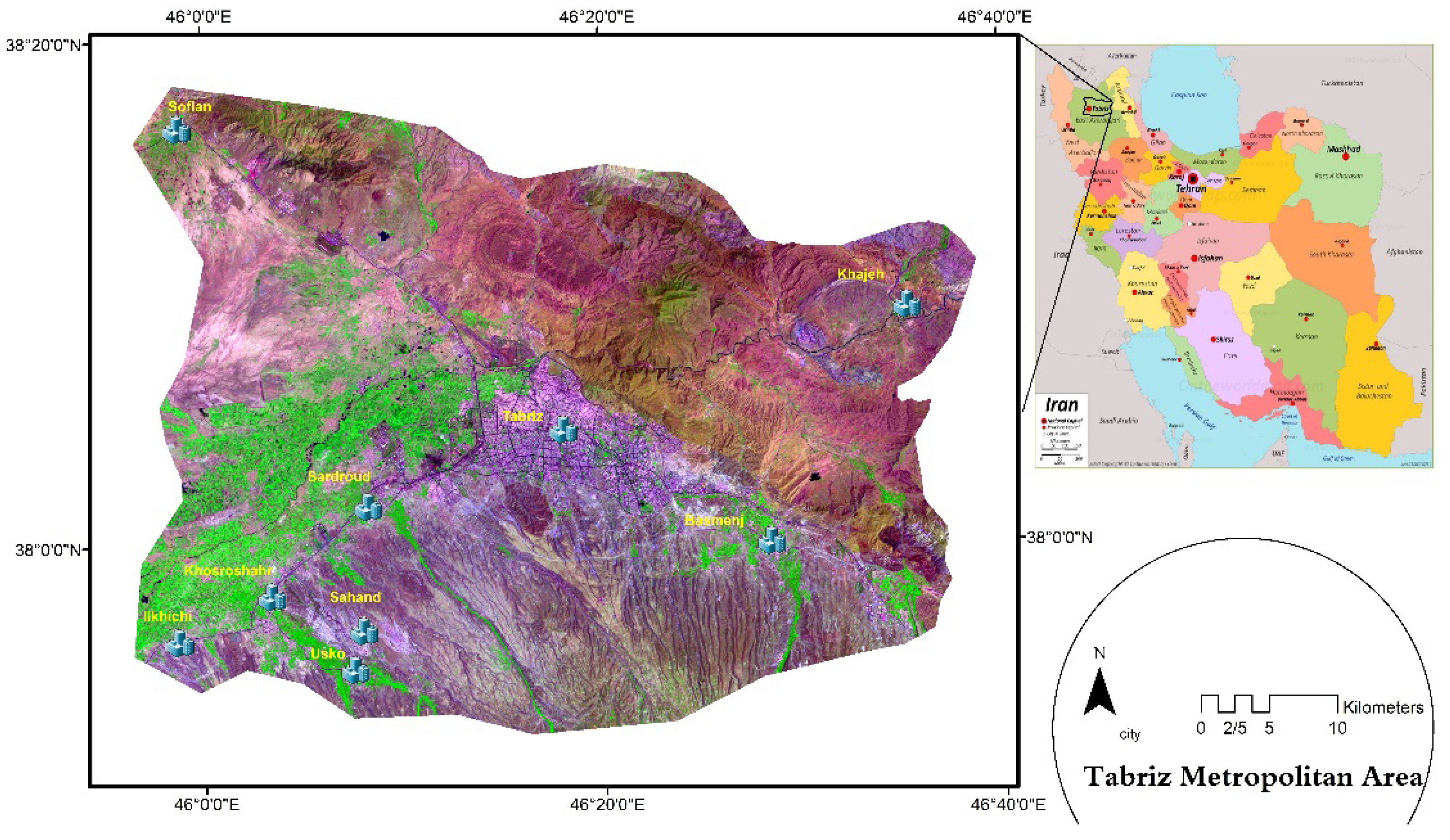
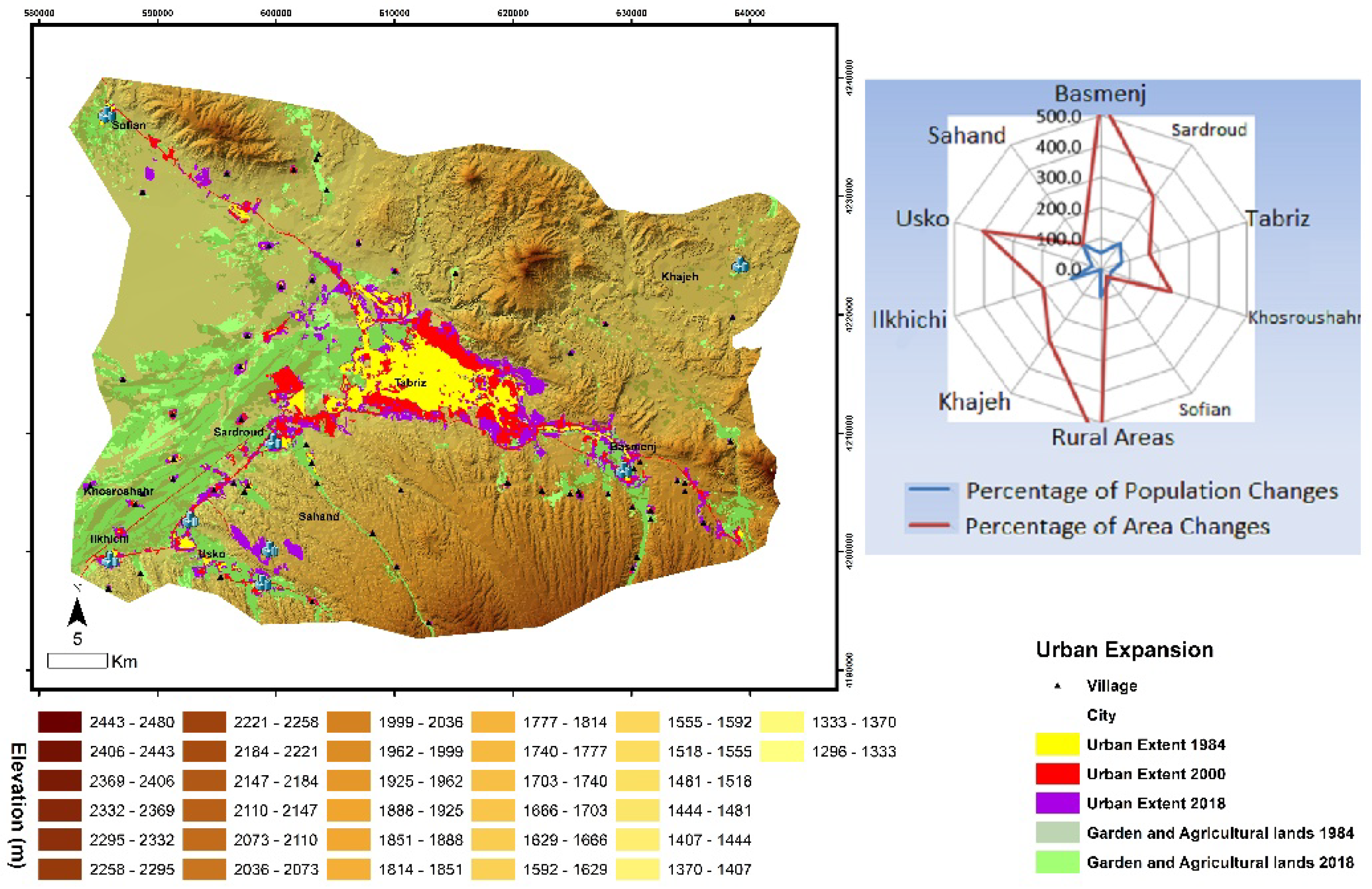
2.1. Study Area
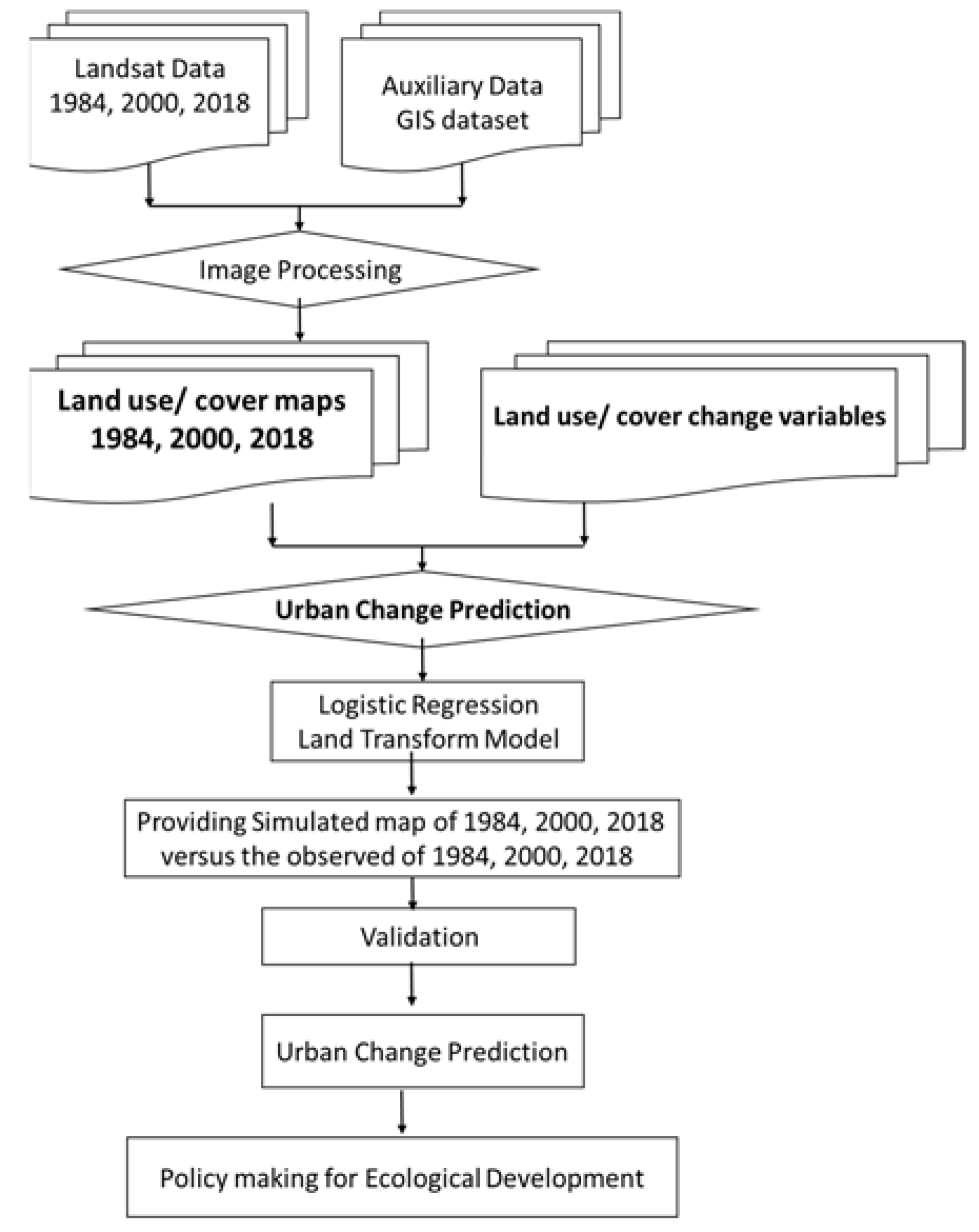
2.2. Methods
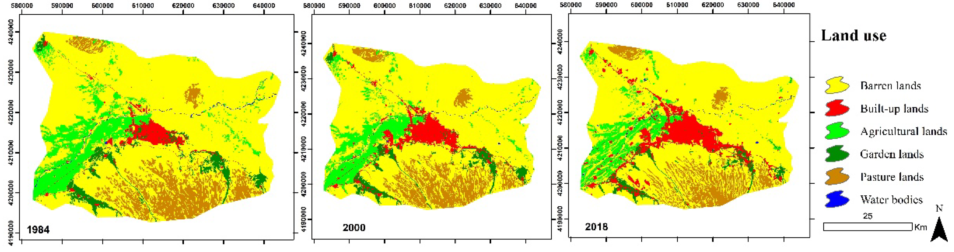
Land-Use/Land-Cover Change Detection
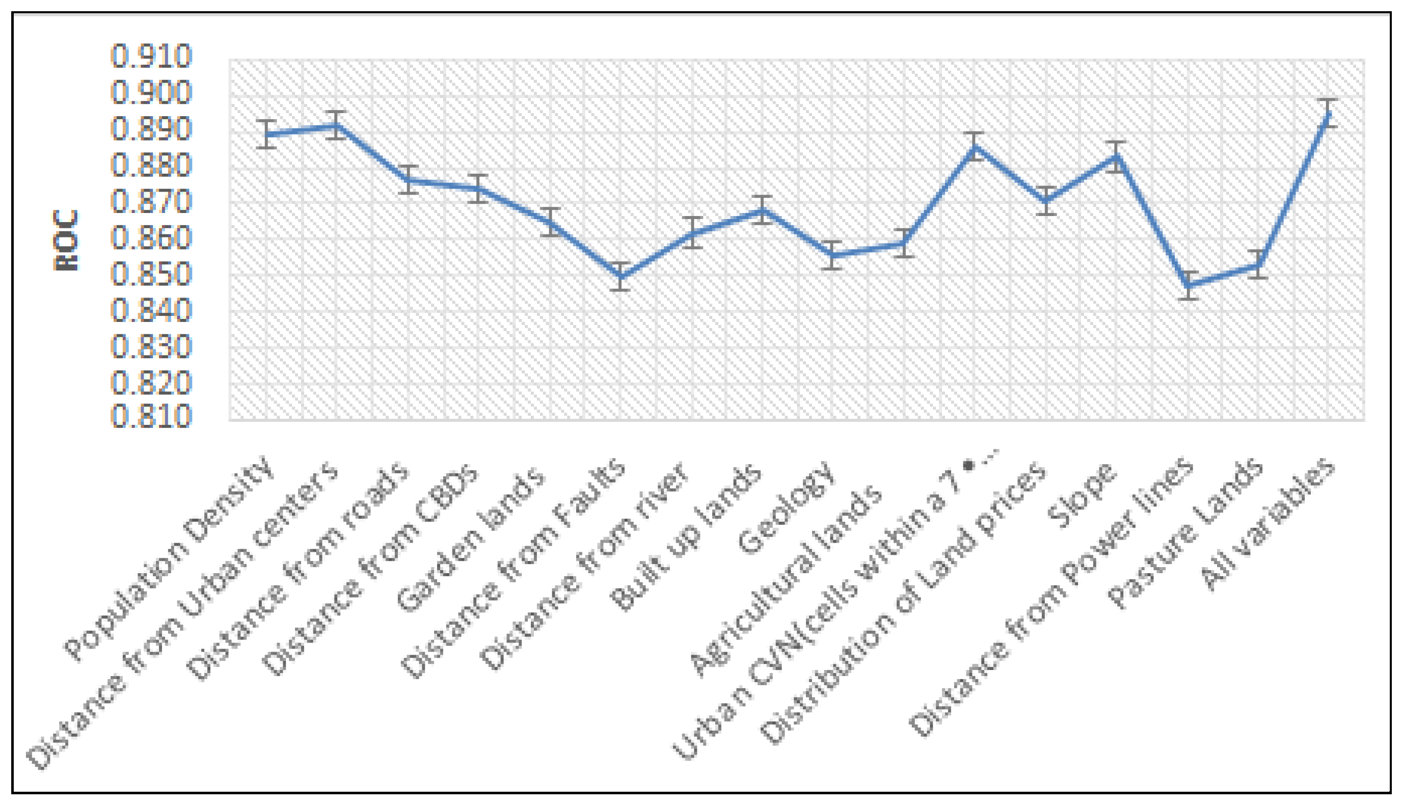
2.3. Logistic Regression Model
Results
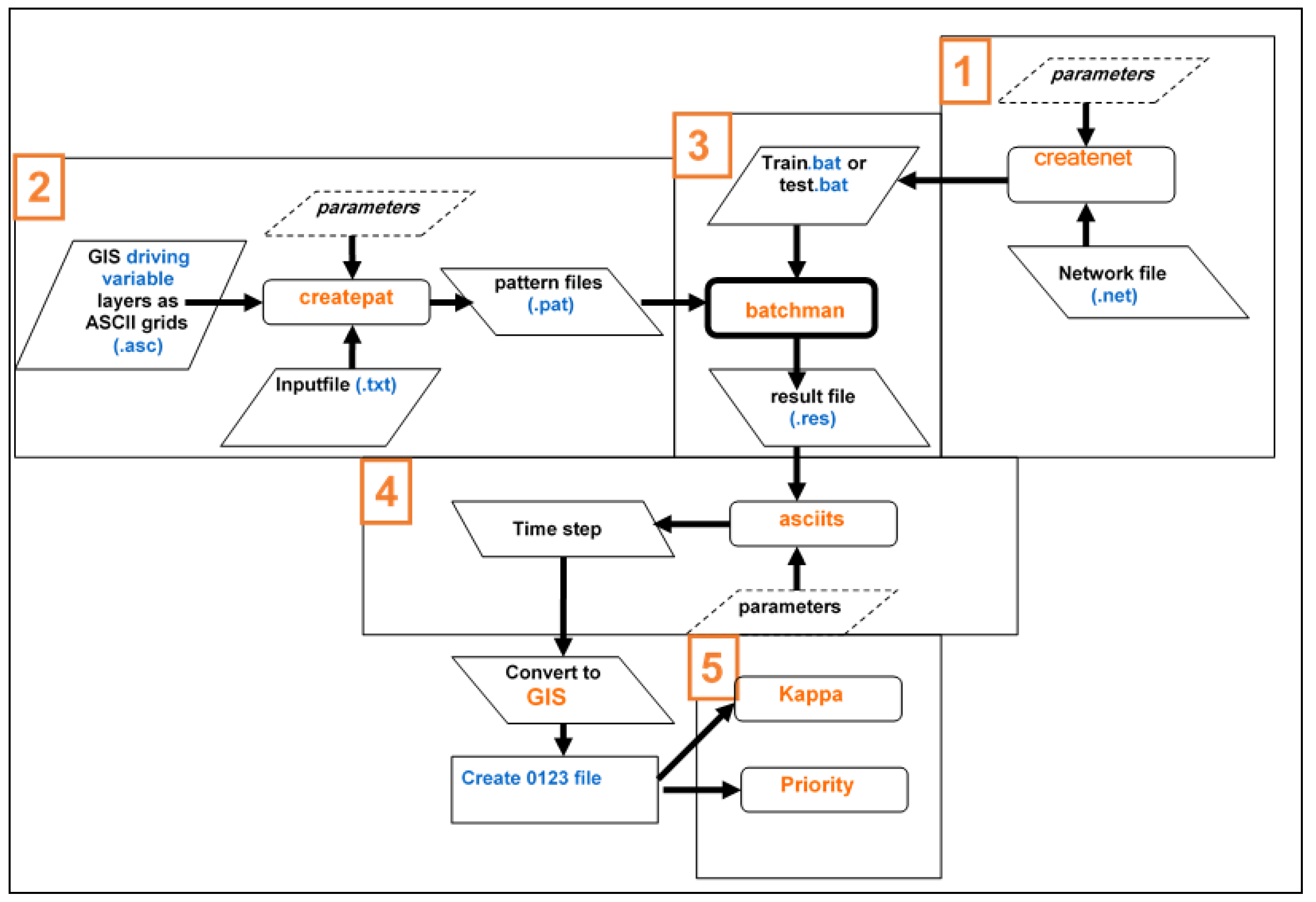
2.4. Land Transformation Model
2.5. TMA Ecological Development Planning
3. Discussion and Conclusions
Author Contributions
Funding
Institutional Review Board Statement
Informed Consent Statement
Data Availability Statement
Conflicts of Interest
References
- Gounaridis, D.; Chorianopoulos, I.; Symeonakis, E.; Koukoulas, S. A Random Forest-Cellular Automata modelling approach to explore future land use/cover change in Attica (Greece), under different socio-economic realities and scales. Sci. Total Environ. 2019, 646, 320–335. [Google Scholar] [CrossRef] [PubMed]
- Vitousek, P.M.; Mooney, H.A.; Lubchenco, J.; Melillo, J.M. Human domination of Earth’s ecosystems. Science 1997, 277, 494–499. [Google Scholar] [CrossRef] [Green Version]
- Jiang, B.; Yao, X. Geospatial Analysis and Modelling of Urban Structure and Dynamics; Springer Science & Business Media: Berlin/Heidelberg, Germany, 2010; Volume 99. [Google Scholar]
- Batisani, N.; Yarnal, B. Uncertainty awareness in urban sprawl simulations: Lessons from a small US metropolitan region. Land Use Policy 2009, 26, 178–185. [Google Scholar] [CrossRef]
- Aguilar, R.; Cristóbal-Pérez, E.J.; Balvino-Olvera, F.J.; de Jesús Aguilar-Aguilar, M.; Aguirre-Acosta, N.; Ashworth, L.; Sanchez-Montoya, G. Habitat fragmentation reduces plant progeny quality: A global synthesis. Ecol. Lett. 2019, 22, 1163–1173. [Google Scholar] [CrossRef] [Green Version]
- Andren, H. Effects of habitat fragmentation on birds and mammals in landscapes with different proportions of suitable habitat: A review. Oikos 1994, 71, 355–366. [Google Scholar] [CrossRef] [Green Version]
- Fahrig, L. Effects of habitat fragmentation on biodiversity. Annu. Rev. Ecol. Evol. Syst. 2003, 34, 487–515. [Google Scholar] [CrossRef] [Green Version]
- Haddad, N.M.; Brudvig, L.A.; Clobert, J.; Davies, K.F.; Gonzalez, A.; Holt, R.D.; Lovejoy, T.E.; Sexton, J.O.; Austin, M.P.; Collins, C.D.; et al. Habitat fragmentation and its lasting impact on Earth’s ecosystems. Sci. Adv. 2015, 1, e1500052. [Google Scholar] [CrossRef] [Green Version]
- Pauchard, A.; Aguayo, M.; Peña, E.; Urrutia, R. Multiple effects of urbanization on the biodiversity of developing countries: The case of a fast-growing metropolitan area (Concepción, Chile). Biol. Conserv. 2006, 127, 272–281. [Google Scholar] [CrossRef]
- Seto, K.C.; Güneralp, B.; Hutyra, L.R. Global forecasts of urban expansion to 2030 and direct impacts on biodiversity and carbon pools. Proc. Natl. Acad. Sci. USA 2012, 109, 16083–16088. [Google Scholar] [CrossRef] [Green Version]
- DeFries, R.S.; Rudel, T.; Uriarte, M.; Hansen, M. Deforestation driven by urban population growth and agricultural trade in the twenty-first century. Nat. Geosci. 2010, 3, 178. [Google Scholar] [CrossRef]
- Li, G.; Lu, D.; Moran, E.; Calvi, M.F.; Dutra, L.V.; Batistella, M. Examining deforestation and agropasture dynamics along the Brazilian TransAmazon Highway using multitemporal Landsat imagery. GIScience Remote Sens. 2019, 56, 161–183. [Google Scholar] [CrossRef]
- Musa, S.I.; Hashim, M.; Reba, M.N.M. Urban growth assessment and its impact on deforestation in Bauchi Metropolis, Nigeria using remote sensing and GIS techniques. ARPN J. Eng. Appl. Sci. 2017, 12, 1907–1914. [Google Scholar]
- Romero, H.; Ihl, M.; Rivera, A.; Zalazar, P.; Azocar, P. Rapid urban growth, land-use changes and air pollution in Santiago, Chile. Atmos. Environ. 1999, 33, 4039–4047. [Google Scholar] [CrossRef]
- Shao, M.; Tang, X.; Zhang, Y.; Li, W. City clusters in China: Air and surface water pollution. Front. Ecol. Environ. 2006, 4, 353–361. [Google Scholar] [CrossRef]
- Song, Y.; Kirkwood, N.; Maksimović, Č.; Zhen, X.; O’Connor, D.; Jin, Y.; Hou, D. Nature based solutions for contaminated land remediation and brownfield redevelopment in cities: A review. Sci. Total Environ. 2019, 663, 568–579. [Google Scholar] [CrossRef]
- Li, B.; Sivapalan, M.; Xu, X. An Urban socio-hydrologic model for exploration of Beijing’s water sustainability challenges and solution spaces. Water Resour. Res. 2019, 55, 5918–5940. [Google Scholar] [CrossRef]
- Walsh, C.J.; Fletcher, T.D.; Burns, M.J. Urban stormwater runoff: A new class of environmental flow problem. PLoS ONE 2012, 7, e45814. [Google Scholar] [CrossRef] [PubMed] [Green Version]
- Morimoto, J.; Negishi, J. Ecological resilience of ecosystems to human impacts: Resilience of plants and animals. Landsc. Ecol. Eng. 2019, 15, 131–132. [Google Scholar] [CrossRef] [Green Version]
- Parsons, A.W.; Rota, C.T.; Forrester, T.; Baker-Whatton, M.C.; McShea, W.J.; Schuttler, S.G.; Millspaugh, J.J.; Kays, R. Urbanization focuses carnivore activity in remaining natural habitats, increasing species interactions. J. Appl. Ecol. 2019, 56, 1894–1904. [Google Scholar] [CrossRef]
- Luo, M.; Lau, N.C. Urban expansion and drying climate in an urban agglomeration of east China. Geophys. Res. Lett. 2019, 46, 6868–6877. [Google Scholar] [CrossRef]
- Mahmood, R.; Pielke Sr, R.A.; Hubbard, K.G.; Niyogi, D.; Dirmeyer, P.A.; McAlpine, C.; Carleton, A.M.; Hale, R.; Gameda, S.; Beltrán-Przekurat, A.; et al. Land cover changes and their biogeophysical effects on climate. Int. J. Climatol. 2014, 34, 929–953. [Google Scholar] [CrossRef]
- Berberoğlu, S.; Akın, A.; Clarke, K.C. Cellular automata modeling approaches to forecast urban growth for Adana, Turkey: A comparative approach. Landsc. Urban Plan. 2016, 153, 11–27. [Google Scholar] [CrossRef]
- Feng, Y.; Liu, Y.; Tong, X.; Liu, M.; Deng, S. Modeling dynamic urban growth using cellular automata and particle swarm optimization rules. Landsc. Urban Plan. 2011, 102, 188–196. [Google Scholar] [CrossRef]
- Alghais, N.; Pullar, D. Modelling future impacts of urban development in Kuwait with the use of ABM and GIS. Trans. GIS 2018, 22, 20–42. [Google Scholar] [CrossRef]
- Shirzadi Babakan, A.; Alimohammadi, A.; Taleai, M. An agent-based evaluation of impacts of transport developments on the modal shift in Tehran, Iran. J. Dev. Eff. 2015, 7, 230–251. [Google Scholar] [CrossRef] [Green Version]
- Zhang, H.; Zeng, Y.; Bian, L.; Yu, X. Modelling urban expansion using a multi agent-based model in the city of Changsha. J. Geogr. Sci. 2010, 20, 540–556. [Google Scholar] [CrossRef]
- Almeida, C.D.; Gleriani, J.; Castejon, E.F.; Soares-Filho, B.S. Using neural networks and cellular automata for modelling intra-urban land-use dynamics. Int. J. Geogr. Inf. Sci. 2008, 22, 943–963. [Google Scholar] [CrossRef]
- Guan, Q.; Wang, L.; Clarke, K.C. An artificial-neural-network-based, constrained CA model for simulating urban growth. Cartogr. Geogr. Inf. Sci. 2005, 32, 369–380. [Google Scholar] [CrossRef] [Green Version]
- Pijanowski, B.C.; Brown, D.G.; Shellito, B.A.; Manik, G.A. Using neural networks and GIS to forecast land use changes: A land transformation model. Comput. Environ. Urban Syst. 2002, 26, 553–575. [Google Scholar] [CrossRef]
- Tayyebi, A.; Pijanowski, B.C.; Tayyebi, A.H. An urban growth boundary model using neural networks, GIS and radial parameterization: An application to Tehran, Iran. Landsc. Urban Plan. 2011, 100, 35–44. [Google Scholar] [CrossRef]
- Thapa, R.B.; Murayama, Y. Scenario based urban growth allocation in Kathmandu Valley, Nepal. Landsc. Urban Plan. 2012, 105, 140–148. [Google Scholar] [CrossRef]
- Hathout, S. The use of GIS for monitoring and predicting urban growth in East and West St Paul, Winnipeg, Manitoba, Canada. J. Environ. Manag. 2002, 66, 229–238. [Google Scholar] [CrossRef]
- Hegazy, I.R.; Kaloop, M.R. Monitoring urban growth and land use change detection with GIS and remote sensing techniques in Daqahlia governorate Egypt. Int. J. Sustain. Built Environ. 2015, 4, 117–124. [Google Scholar] [CrossRef] [Green Version]
- Moghadam, H.S.; Helbich, M. Spatiotemporal urbanization processes in the megacity of Mumbai, India: A Markov chains-cellular automata urban growth model. Appl. Geogr. 2013, 40, 140–149. [Google Scholar] [CrossRef]
- Ozturk, D. Urban growth simulation of Atakum (Samsun, Turkey) using cellular automata-Markov chain and multi-layer perceptron-Markov chain models. Remote Sens. 2015, 7, 5918–5950. [Google Scholar] [CrossRef] [Green Version]
- Tang, J.; Wang, L.; Yao, Z. Spatio-temporal urban landscape change analysis using the Markov chain model and a modified genetic algorithm. Int. J. Remote Sens. 2007, 28, 3255–3271. [Google Scholar] [CrossRef]
- Huang, B.; Xie, C.; Tay, R.; Wu, B. Land-use-change modeling using unbalanced support-vector machines. Environ. Plan. B Plan. Des. 2009, 36, 398–416. [Google Scholar] [CrossRef] [Green Version]
- Karimi, F.; Sultana, S.; Babakan, A.S.; Suthaharan, S. An enhanced support vector machine model for urban expansion prediction. Comput. Environ. Urban Syst. 2019, 75, 61–75. [Google Scholar] [CrossRef]
- Mirbagheri, B.; Alimohammadi, A. Integration of local and global support vector machines to improve urban growth modelling. ISPRS Int. J. Geo-Inf. 2018, 7, 347. [Google Scholar] [CrossRef] [Green Version]
- Rienow, A.; Goetzke, R. Supporting SLEUTH–Enhancing a cellular automaton with support vector machines for urban growth modeling. Comput. Environ. Urban Syst. 2015, 49, 66–81. [Google Scholar] [CrossRef]
- Addae, B.; Oppelt, N. Land-use/land-cover change analysis and urban growth modelling in the Greater Accra Metropolitan Area (GAMA), Ghana. Urban Sci. 2019, 3, 26. [Google Scholar] [CrossRef]
- Bekalo, M.T. Spatial Metrics and Landsat Data for Urban Landuse Change Detection: Case of Addis Ababa, Ethiopia. Doctoral Dissertation, Universitat Jaume I, Castellon, Spain, 2009. [Google Scholar]
- Aarthi, A.D.; Gnanappazham, L. Comparison of urban growth modeling using deep belief and neural network based cellular automata model—A case study of Chennai Metropolitan area, Tamil Nadu, India. J. Geogr. Inf. Syst. 2019, 11, 1–16. [Google Scholar] [CrossRef] [Green Version]
- Sejati, A.W.; Buchori, I.; Rudiarto, I. The spatio-temporal trends of urban growth and surface urban heat islands over two decades in the Semarang Metropolitan Region. Sustain. Cities Soc. 2019, 46, 101432. [Google Scholar] [CrossRef]
- Wang, J.; Maduako, I.N. Spatio-temporal urban growth dynamics of Lagos Metropolitan Region of Nigeria based on Hybrid methods for LULC modeling and prediction. Eur. J. Remote Sens. 2018, 51, 251–265. [Google Scholar] [CrossRef] [Green Version]
- Xia, C.; Zhang, A.; Wang, H.; Zhang, B. Modeling urban growth in a metropolitan area based on bidirectional flows, an improved gravitational field model, and partitioned cellular automata. Int. J. Geogr. Inf. Sci. 2019, 33, 877–899. [Google Scholar] [CrossRef]
- Gong, J.; Hu, Z.; Chen, W.; Liu, Y.; Wang, J. Urban expansion dynamics and modes in metropolitan Guangzhou, China. Land Use Policy 2018, 72, 100–109. [Google Scholar] [CrossRef]
- Siddiqui, A.; Siddiqui, A.; Maithani, S.; Jha, A.; Kumar, P.; Srivastav, S. Urban growth dynamics of an Indian metropolitan using CA Markov and Logistic Regression. Egypt. J. Remote Sens. Space Sci. 2018, 21, 229–236. [Google Scholar] [CrossRef]
- Alaei Moghadam, S.; Karimi, M.; Habibi, K. Modelling urban growth incorporating spatial interactions between the cities: The example of the Tehran metropolitan region. Environ. Plan. B Urban Anal. City Sci. 2018, 47, 1047–1064. [Google Scholar] [CrossRef]
- Sun, X.; Crittenden, J.C.; Li, F.; Lu, Z.; Dou, X. Urban expansion simulation and the spatio-temporal changes of ecosystem services, a case study in Atlanta Metropolitan area, USA. Sci. Total Environ. 2018, 622, 974–987. [Google Scholar] [CrossRef]
- Pandey, B.; Joshi, P.; Singh, T.; Joshi, A. Modelling spatial patterns of urban growth in Pune Metropolitan Region, India. In Applications and Challenges of Geospatial Technology; Springer: Berlin/Heidelberg, Germany, 2019; pp. 181–203. [Google Scholar]
- Thapa, R.B.; Murayama, Y. Urban growth modeling of Kathmandu metropolitan region, Nepal. Comput. Environ. Urban Syst. 2011, 35, 25–34. [Google Scholar] [CrossRef]
- Puertas, O.L.; Henríquez, C.; Meza, F.J. Assessing spatial dynamics of urban growth using an integrated land use model. Application in Santiago Metropolitan Area, 2010–2045. Land Use Policy 2014, 38, 415–425. [Google Scholar] [CrossRef]
- Hilbe, J.M. Practical Guide to Logistic Regression; Chapman and Hall/CRC: London, UK, 2016. [Google Scholar]
- Li, J.; Dong, S.; Li, Y.; Li, Z.; Wang, J. Driving force analysis and scenario simulation of urban land expansion in Ningxia-Inner Mongolia area along the Yellow River. J. Nat. Resour. 2015, 30, 1472–1485. [Google Scholar]
- Mahiny, A.S.; Turner, B.J. Modeling past vegetation change through remote sensing and GIS: A comparison of neural networks and logistic regression methods. In Proceedings of the 7th International Conference on Geocomputation, University of Southampton, Southampton, UK, 8–10 September 2003. [Google Scholar]
- Hill, T.; Lewicki, P. Statistics Methods and Applications; StatSoft: Washington, DC, USA, 2007. [Google Scholar]
- Hu, Z.; Lo, C. Modeling urban growth in Atlanta using logistic regression. Comput. Environ. Urban Syst. 2007, 31, 667–688. [Google Scholar] [CrossRef]
- Aldrich, J.H.; Nelson, F.D.; Adler, E.S. Linear Probability, Logit, and Probit Models; Sage: Thousand Oaks, CA, USA, 1984. [Google Scholar]
- Clark, W.; Hoskings, P. Statistical Methods for Geographers; John Wiley and Sons: New York, NY, USA, 1986. [Google Scholar]
- Menard, S. Applied Logistic Regression Analysis; Sage: Thousand Oaks, CA, USA, 2002; Volume 106. [Google Scholar]
- Xu, T.; Gao, J.; Coco, G. Simulation of urban expansion via integrating artificial neural network with Markov chain–cellular automata. Int. J. Geogr. Inf. Sci. 2019, 33, 1960–1983. [Google Scholar] [CrossRef]
- Pijanowski, B.C.; Tayyebi, A.; Doucette, J.; Pekin, B.K.; Braun, D.; Plourde, J. A big data urban growth simulation at a national scale: Configuring the GIS and neural network based land transformation model to run in a high performance computing (HPC) environment. Environ. Model. Softw. 2014, 51, 250–268. [Google Scholar] [CrossRef]
- Abedini, A.; Khalili, A. Determining the capacity infill development in growing metropolitans: A case study of Urmia city. J. Urban Manag. 2019, 8, 316–327. [Google Scholar] [CrossRef]
- Adhvaryu, B.; Rathod, V. Estimating housing infill potential: Developing a case for floorspace pooling in Ahmedabad, India. Plan. Pract. Res. 2019, 34, 305–317. [Google Scholar] [CrossRef]
- Heymans, A.; Breadsell, J.; Morrison, G.M.; Byrne, J.J.; Eon, C. Ecological urban planning and design: A systematic literature review. Sustainability 2019, 11, 3723. [Google Scholar] [CrossRef] [Green Version]
- Warren-Kretzschmar, B.; von Haaren, C. Design in landscape planning solutions. In Landscape Planning with Ecosystem Services; Springer: Berlin/Heidelberg, Germany, 2019; pp. 453–460. [Google Scholar]
- Gyan, E. Green belt as a tool for containing urban sprawl: Exploring best practices in Germany. Book of Abstracts. In Proceedings of the 6th Fábos Conference on Lanscape and Greenway Planning, Amherst, MA, USA, 29–30 March 2019. [Google Scholar]
- Home, R.; Lewis, O.; Bauer, N.; Fliessbach, A.; Frey, D.; Lichtsteiner, S.; Moretti, M.; Tresch, S.; Young, C.; Zanetta, A.; et al. Effects of garden management practices, by different types of gardeners, on human wellbeing and ecological and soil sustainability in Swiss cities. Urban Ecosyst. 2019, 22, 189–199. [Google Scholar] [CrossRef]
- Park, Y.S.; Lek, S. Artificial neural networks: Multilayer perceptron for ecological modeling. In Developments in Environmental Modelling; Elsevier: Amsterdam, The Netherlands, 2016; Volume 28, pp. 123–140. [Google Scholar]
- Chaudhuri, G.; Clarke, K. The SLEUTH land use change model: A review. Environ. Resour. Res. 2013, 1, 88–105. [Google Scholar]
- Eyelade, D.; Clarke, K.C.; Ijagbone, I. Impacts of spatiotemporal resolution and tiling on SLEUTH model calibration and forecasting for urban areas with unregulated growth patterns. Int. J. Geogr. Inf. Sci. 2022, 36, 1037–1058. [Google Scholar] [CrossRef]


| Data | Source | Resolution (m) | Date |
|---|---|---|---|
| Landsat 5 TM | US Geological Survey | 30 | 10 July 1984 |
| Landsat 7 ETM+ | US Geological Survey | 30,15 (PAN) | 31 August 2000 |
| Landsat 8 OLI | US Geological Survey | 30,15 (PAN) | 8 July 2018 |
| Land Use | 1984 | 2000 | 2018 | 1984–2000 | 2000–2018 | 1984–2018 | |||
|---|---|---|---|---|---|---|---|---|---|
| Area | Total% | Area | Total% | Area | Total% | Variation | Variation | Variation | |
| Barren lands | 151,962.57 | 68.85 | 149,223.51 | 67.60 | 147,051.99 | 66.62 | −1.80 | −1.46 | −3.23 |
| Built-up lands | 7220.34 | 3.27 | 14,027.58 | 6.35 | 22,346.82 | 10.12 | 94.27 | 59.30 | 209.50 |
| Agricultural lands | 25,369.83 | 11.49 | 23,259.42 | 10.53 | 22,489.02 | 10.18 | −8.32 | −3.31 | −11.36 |
| Garden lands | 10,242.63 | 4.65 | 9094.86 | 4.12 | 6653.43 | 3.01 | −11.21 | −26.84 | −35.04 |
| Pasture lands | 25,248.15 | 11.44 | 24,669.99 | 11.17 | 21,583.80 | 9.77 | −2.29 | −12.51 | −14.51 |
| Water bodies | 669.24 | 0.30 | 437.40 | 0.19 | 587.700 | 0.26 | −34.64 | 34.36 | 12.18 |
| 1984 | 2000 | 2018 | |
|---|---|---|---|
| Overall Accuracy | 93.6 | 95.3 | 96.4 |
| Kappa Coefficient | 0.89 | 0.91 | 0.94 |
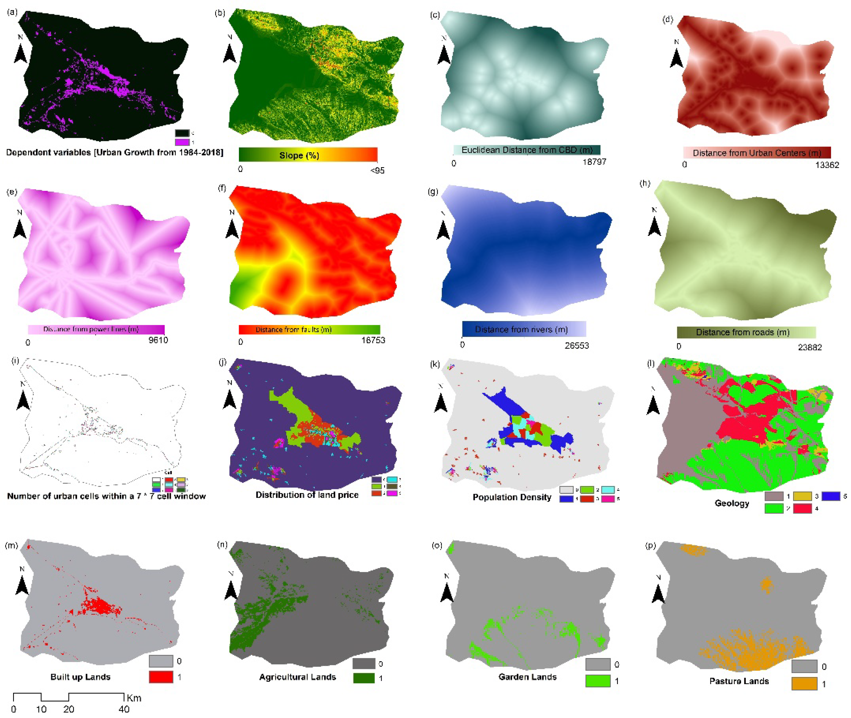
| Variable Description | Source and Description | Nature of Variable |
|---|---|---|
| Dependent variable Urban growth from 1984 to 2018 | Subtraction of the Boolean Urban areas for 1984 from 2018 (classified images); 0—no urban growth; 1—urban growth | Dichotomous |
| Slope | Slope in percent | Continuous |
| Population density | Population density (person/ha) | Continuous |
| Distance from commercial centers | Euclidean distance from CBD(m) | Continuous |
| Distance from roads | Distance to the nearest major road (m) | Continuous |
| Distance from urban centers | Euclidean distance to the urban region (m) | Continuous |
| Distance from power lines | Euclidean distance from power lines (m) | Continuous |
| Distance from rivers | Euclidean distance from rivers (m) | Continuous |
| Distance from faults | Euclidean distance from faults (m) | Continuous |
| Urban CVN (center versus neighbor) | Number of urban cells within a 7 · 7 cell window (ranging from 0 to 8) | Ranging from 0 to 8 |
| Geology | The degree of hardness for lithological structures | Continuous |
| Barren lands | 1—bare land; 0—not bare land | Design |
| Garden lands | 1—garden land; 0—not garden land | Design |
| Agriculture lands | 1—agriculture land; 0—not agriculture land | Design |
| Pasture lands | 1—pasture land; 0—not pasture land | Design |
| Built up lands | 1—built-up lands; 0—not built-up lands | Design |
| Distribution of land price | Spatial distribution of land price | Continuous |
| 1984–2000 | 2000–2018 | 1984–2018 | |||
|---|---|---|---|---|---|
| ROC | Pseudo-R2 | ROC | Pseudo-R2 | ROC | Pseudo-R2 |
| 0.86 | 0.78 | 0.82 | 0.74 | 0.89 | 0.79 |
| Step 14 | −2 Log Likelihood | Cox & Snell R2 | Nagelkerke R2 | Pseudo R2 |
|---|---|---|---|---|
| 26391.79 | 0.39 | 0.61 | 0.79 |
| B a | S.E. b | Wald c | Df d | Sig. e | Exp(B) f | 95% C.I. for EXP(B) g | ||
|---|---|---|---|---|---|---|---|---|
| Lower | Upper | |||||||
| Constant | −2.867 | 0.030 | 8861.936 | 1 | 0.000 | 0.507 | ||
| Built-up lands | −0.26 | 0.011 | 6.178 | 1 | 0.000 | 0.974 | 0.954 | 0.994 |
| Agriculture lands | −0.80 | 0.012 | 45.186 | 1 | 0.000 | 0.924 | 0.902 | 0.945 |
| Land prices | −0.155 | 0.021 | 53.915 | 1 | 0.000 | 0.856 | 0.822 | 0.893 |
| Pasture lands | −0.137 | 0.010 | 183.715 | 1 | 0.013 | 0.872 | 0.855 | 0.890 |
| Garden lands | −0.131 | 0.010 | 180.805 | 1 | 0.000 | 0.877 | 0.861 | 0.894 |
| Dist f roads | 0.328 | 0.010 | 1067.199 | 1 | 0.000 | 1.389 | 1.362 | 1.416 |
| Dist f urban | 1.519− | 0.050 | 922.745 | 1 | 0.000 | 0.219 | 0.199 | 0.242 |
| Dist f CBDs | −0.206 | 0.017 | 147.599 | 1 | 0.000 | 0.814 | 0.788 | 0.842 |
| Dist f power lines | −0.39 | 0.012 | 10.334 | 1 | 0.001 | 0.962 | 0.940 | 0.985 |
| Geology | −0.71 | 0.011 | 45.219 | 1 | 0.013 | 0.932 | 0.913 | 0.951 |
| Dist f faults | −0.53 | 0.011 | 21.772 | 1 | 0.000 | 1.054 | 1.031 | 1.077 |
| Urban CVN | 0.407 | 0.013 | 1028.951 | 1 | 0.000 | 0.665 | 0.649 | 0.682 |
| Dist f rivers | −0.057 | 0.014 | 17.289 | 1 | 0.013 | 0.944 | 0.919 | 0.970 |
| Slope | −0.380 | 0.029 | 171.274 | 1 | 0.000 | 0.684 | 0.646 | 0.724 |
| Population density | 1.105 | 0.009 | 13548.603 | 1 | 0.000 | 3.019 | 2.964 | 3.076 |
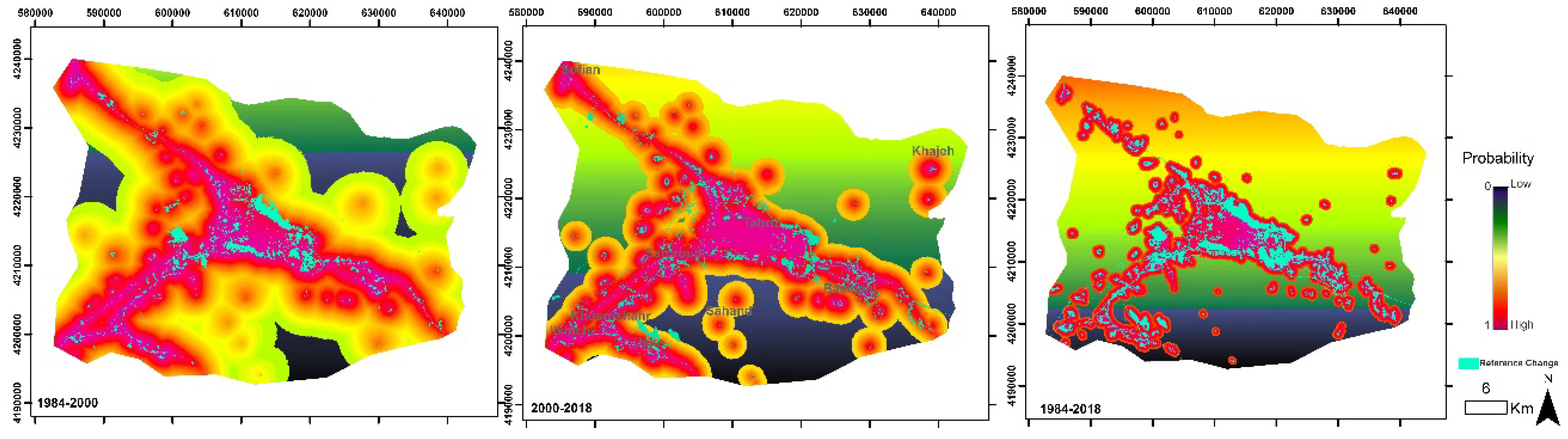
| 1984–2000 | 2000–2018 | 1984–2018 | ||||||
|---|---|---|---|---|---|---|---|---|
| RMS | Kappa | PCM | RMS | Kappa | PCM | RMS | Kappa | PCM |
| Cycle 9300 | Cycle 8600 | Cycle 8000 | ||||||
| 0.0197233 | 0.865437 | 85.871426 | 0.0186641 | 0.853461 | 86.842313 | 0.0189534 | 0.844434 | 87.831315 |
| Advantages | Disadvantages |
|---|---|
| Logistic regression is easy to implement and interpret and very efficient to train (Terrset). | If the number of observations is less than the number of features, logistic regression should not be used and may lead to overfitting. |
| It makes no assumptions about distributions of classes in feature the space (Table 4). | It constructs linear boundaries. |
| It can easily extend to multiple classes (multinomial regression) and a natural probabilistic view of class predictions (lack of necessity). | The major limitation of logistic regression is the assumption of linearity between the dependent variable and the independent variables. |
| It not only provides a measure of the appropriatenes of a predictor (coefficient size) but also its direction of association (positive or negative) (Table 6 and Table 7). | It can only be used to predict discrete functions. Hence, the dependent variable of logistic regression is bound to the discrete number set. |
| It can rapidly classify unknown records. | Non-linear problems cannot be solved with logistic regression because it has a linear decision surface. Linearly separable data are rarely found in real-world scenarios. |
| Accuracy on many simple datasets and performs well when the dataset is linearly separable. | Logistic regression requires average or absent multicollinearity between independent variables. |
| It can interpret model coefficients as indicators of feature importance (Table 7). | It is difficult to obtain complex relationships using logistic regression. More powerful and compact algorithms such as neural networks can easily outperform logistic regression. |
| Logistic regression is less inclined to overfit, but it can overfit in high dimensional datasets. Regularization (L1 and L2) techniques may be considered to avoid overfitting in such scenarios (Table 6). | In linear regression, independent and dependent variables are related linearly. However, logistic regression requires that independent variables be linearly related to the log odds (log(p/(1 − p)). |
| Advantages | Disadvantages |
|---|---|
| Can be applied to complex non-linear problems. | It is not known to what extent each independent variable is affected by the dependent variable. Computations are difficult and time-consuming. |
| Works well with large input data (TMA). | The proper functioning of the model depends on the quality of the training data. |
| Provides quick predictions after training (Figure 9). | If the model does not work properly, generalization problems arise. |
| Same accuracy ratio can be achieved, even with small datasets. |
| City | Land-Use Type | Area (Ha) | Function |
|---|---|---|---|
| Tabriz | Incompatible land uses | 702 | Reducing environmental pollution |
| Deteriorated textures | 420 | The revitalization of the city | |
| One-story housing units | 2462 | Infill development (compact city strategy) | |
| Vacant lands | 6043 | Limiting urban spatial polarization with the strengthening of new centers |
| City | Type | Direction | Length (Km) | Function |
|---|---|---|---|---|
| Tabriz | Artificial Green Belt | Northern | 12.4 | Stabilization of the urban development and limiting it toward the Tabriz fault |
| Artificial Green Belt | Southern | 21.3 | Stabilization of the urban area and reducing air pollutants from industrial land use sources | |
| Natural Green Belt | Western | 16.1 | To preserve agricultural land and stop the spread of villages in the west of Tabriz | |
| Basmenj | Natural Green Belt | Southern | 6.3 | Preservation of southern gardens of Basmenj |
| Sardroud | Natural Green Belt | Southern | 4.4 | Protection of southern gardens of Sardroud from rural development |
| Khosroshahr | Natural Green Belt | Eastern | 4 | Prevention of rural–urban integration in Khosrowshahr |
| Natural green bow | Northern–Eastern | 7.3 | Preservation of garden lands in Khosrowshahr | |
| Usko | Natural Green Belt | Eastern–Western–Southern | 13.4 | Prevention of rural–urban integration in Usko |
| Natural green bow | Eastern–Western | 6.4 | Preservation of garden lands in Usko |
Publisher’s Note: MDPI stays neutral with regard to jurisdictional claims in published maps and institutional affiliations. |
© 2022 by the authors. Licensee MDPI, Basel, Switzerland. This article is an open access article distributed under the terms and conditions of the Creative Commons Attribution (CC BY) license (https://creativecommons.org/licenses/by/4.0/).
Share and Cite
Mahmoudzadeh, H.; Abedini, A.; Aram, F. Urban Growth Modeling and Land-Use/Land-Cover Change Analysis in a Metropolitan Area (Case Study: Tabriz). Land 2022, 11, 2162. https://doi.org/10.3390/land11122162
Mahmoudzadeh H, Abedini A, Aram F. Urban Growth Modeling and Land-Use/Land-Cover Change Analysis in a Metropolitan Area (Case Study: Tabriz). Land. 2022; 11(12):2162. https://doi.org/10.3390/land11122162
Chicago/Turabian StyleMahmoudzadeh, Hassan, Asghar Abedini, and Farshid Aram. 2022. "Urban Growth Modeling and Land-Use/Land-Cover Change Analysis in a Metropolitan Area (Case Study: Tabriz)" Land 11, no. 12: 2162. https://doi.org/10.3390/land11122162
APA StyleMahmoudzadeh, H., Abedini, A., & Aram, F. (2022). Urban Growth Modeling and Land-Use/Land-Cover Change Analysis in a Metropolitan Area (Case Study: Tabriz). Land, 11(12), 2162. https://doi.org/10.3390/land11122162