Abstract
This study examines the long-term impact of energy production and economic growth on the environment using data on real GDP, energy production (and its subcomponents), carbon dioxide emissions, and real foreign trade. The datasets contain 99 countries that are classified into seven regions and analyzed by using MG, AMG, and CCEMG estimators. Estimates reflect that economic growth increases environmental pollution while foreign trade decreases it in all selected regions. In analyzing the conservation and neutrality hypotheses, we found that the conservation hypothesis was successfully verified for the global panel, Europe, and Africa, whereas the former was verified in North America, the Middle East, and the Asia Pacific regions. The study suggests focusing on renewable energy production policies to sustain the current growth pace.
1. Introduction
For more than two decades, the rising threat of climate change and global warming has been a primary global concern. Available literature argues that increasing carbon emissions significantly contributes to environmental pollution. Investigation of the energy-emissions relationship is vital as these emissions will rise even more due to the rise in global population, and energy usage will also rise as a consequence. Consumption and production of energy from non-renewable sources like coal, crude oil, and natural gas increase environmental pollution and degradation [1,2]. Energy is an essential tool for performing economic activities and plays a crucial role in the sustainable development of economies. Economic productivity is powered by energy production and consumption and used as the yardstick for measuring the development status of nations. Energy enterprises are concerned with almost all the sustainable development goals, ranging from water supply and food, economic growth (EG) and jobs, wellbeing, industrialization, eradication of poverty, responsible consumption and production, and climate change mitigation [3].
There is a close association between energy, EG, and the environment. This nexus has received significant attention over the years from researchers and policy analysts. Due to the adverse effects of fossil fuels like coal energy, crude oil, and natural gas on the environment, the demand for alternative energy sources like hydropower, wind and solar, and biofuels and waste is increasing. Along with increasing the ratio of renewable energy (RE) by installed capacity, it is also necessary for countries to emphasize the RE infrastructure [4]. Energy generation from non-exhaustible sources is the best substitute for non-RE as it is clean and produces less CO2 emissions [5,6]. RE has become an adequate substitute for fossil fuels and opens the way toward a sustainable environment and EG [7]. The demand for solar and wind, biofuels and waste, hydropower, and biomass is increasing globally [8]. To use and fast-track the accessibility of RE, United Nations Organization also emphasizes developing and promoting RE sources as a business [9]. Literature is divided into different strands in this regard and found positive [10], negative [11], or no impact [12] of the energy on the environment, respectively.
The above discussion highlights the worth of the relationship between the environment and renewable energy sources. Countries with higher growth rates may develop and promote more RE production and consumption [13]. Like economic growth, foreign trade is closely linked with energy and carbon emissions. Trade has a noteworthy influence on the environment and boosts EG [14]. In recent years, the total volume of RE trading products has been increasing globally. Foreign trade can play a crucial role in greening and promoting the energy sector through transmitting RE technologies. At the same time, exports may encourage production and stimulate RE consumption, leading to a sustainable environment and EG. In this way, foreign trade is fascinating in explaining the impact of energy production and EG on environmental degradation (ED).
Some critical gaps perceived in the available literature give the motivation for this study. A recent relevant study by Chen et al. [4] assessed the impact of renewable and non-RE production on EG, emissions, and foreign trade for a single country. However, such a relationship may be driven by panel data and more countries in the form of groups or regions, which is essential for policy analysts. Another study by Rahman et al. [15] focused on disaggregating the level of energy production and consumption with the relationship of EG. Afterward, Antonakakis et al. [16] studied the demand side of energy with its subcomponents to inspect the causal association of energy consumption, EG, and CO2 emissions while ignoring the supply side of energy. Most relevant existing studies used conventional econometric techniques, i.e., first-generation, to examine such relationships while ignoring cross-sectional dependence (CSD) in the panel data.
This paper analyzes the impact of disaggregated energy (production side) on ED. The empirical issue can emerge when the variables do not share the same level of aggregation. Partially-disaggregated analysis on one energy type related to the energy-environment association may yield misleading findings and not state the potential impacts of other energy types. Therefore, the authors included all energy input components from exhaustible and non-exhaustible sources as the independent variables. Most of the previous studies conglomerate the coal mining and coking sector into a single sector and the petroleum extraction sector and refined oil sector into another, which may bias the policy simulation results because the feedstock input of crude oil or coal will be measured as the energy input. Petroleum and extraction of natural gas extraction activities are heterogeneous, and hence disaggregating this sector is necessary for policy analysis. Many researchers disaggregate the petroleum and natural gas extraction sectors into a petroleum extraction and a natural gas extraction sector solely based on their physical shares in primary energy consumption. This disaggregation technique produces inaccurate results, as the two products output structures in the production process and distribution structures differ substantially. Unlike the existing literature, which failed to disaggregate non-RE and RE from electric power, this article includes coal, crude oil, and natural gas as the sources of non-RE, and hydropower, wind and solar, biofuels and waste as the sources of non-RE, separately.
Against this background, three main silent attributes differentiate this article from the preceding and contribute to the existing literature in the following aspects. First, despite the considerable research on the energy-environment nexus, there is not even a single study with such an exciting combination of variables. The study considers carbon emissions, energy production from non-RE and RE sources, real trade, and economic growth. There is no consensus regarding the impact of GHG emission, energy production from different sectors and sources, and economic growth as the energy production side disaggregated panel analysis based on different energy sectors is missing in the current literature. This article will push the frontiers of energy-environment knowledge by quantifying the said nexus by taking global-level data. Second, considering the differences in 7 regions with 99 countries, we identified the deriving issues of carbon emissions across the regions. Hence, we built a very inclusive dataset of 99 countries for energy production, EG, and the environment from 1990–2017. Energy production was disaggregated into seven subcomponents, i.e., total energy production, coal, crude oil, natural gas, wind and solar, hydropower, biofuels, and waste. Foreign trade was taken as a variable to control the omitted variable’s biasedness. We classified countries into eight regions set by International Energy Agency (IEA): the Global panel, North America, Central, and South America, Europe, Eurasia, Africa, Middle East, and Asia Pacific.
Existing studies have analyzed the role of renewable and non-RE consumption on ED while ignoring the production side that the study considers. This study’s results will help policymakers formulate policies regarding CO2 emissions mitigation. Third, we provide a robust analysis of causal links using second-generation methods instead of conventional econometric techniques, which do not considers the slope homogeneity and CSD across the panels. We investigated the impact of energy production and EG on CO2 emissions using second-generation Mean Group (MG), Augmented Mean Group (AMG), and Common correlated effects mean group (CCEMG) regression techniques. Also, we examine the causality among the variables using the D-H causality test.
This section briefly discussed the background of the study. Section 2 presents a brief literature review, Section 3 presents the empirical methodology, including the data and empirical model, as well as estimation techniques. Section 4 presents the empirical findings and discussion regarding the study results. The last section presents the summary, and concluding remarks are presented.
2. Literature Review
The findings among previous studies remain dissimilar and conflicting. Jebli et al. [17] analyzed 102 countries based on income groups. Their study took CO2 emissions, per capita real GDP, REC, service value-added, and industrial value-added. The results showed that RE consumption positively affects service value-added and industrial value-added. Antonakakis et al. [16] found that energy consumption with its subcomponents has heterogeneous effects on EG and carbon emission in various groups of nations. For China, Rahman et al. [15] used data from 1981 to 2016 and estimated that the consumption and production of coal, oil, and natural gas have a positive impact on GDP. Rahman and Velayutham [18] used FMOLS, DOLS, and D–H causality methods. Their study estimated the positive impacts of nonrenewable, RE consumption, and capital formation on EG. Another study for China by Chen et al. [4] used RE and non-RE production, per capita CO2, GDP, and foreign trade and found a long-term relationship among the selected variables. For instance, Maji et al. [19] concluded that RE consumption slows down EG with the use of inefficient and unclean resources. A study by Dong et al. [20] for six regions by IEA found that the EG and population positively affect carbon emissions at the global and regional levels. For Latin America and the Caribbean emerging markets and developing economies, Le and Bao [21] conducted a study, and the results of the MG, AMG, and CCEMG estimations claimed that nonrenewable and RE consumption positively affects EG.
Sarkodie and Strezov [22] used FMOLS, DOLS, and Canonical cointegration methods and claimed that more shares of RE penetration decrease while more shares of non-RE increase the level of emissions. Moreover, Sarkodie et al. [23] examined the inverse U-shaped relationship between carbon emission and EG. For a case study of Iran by Ahmad and Du’s [24] used FMOLS, DOLS, and ARDL and results showed that emission and energy production have positive impacts on EG. Further, domestic investment is more important for EG than foreign investment. Przychodzen and Przychodzen [25] found that higher EG, government debt, and higher employment rates stimulate RE production. For Italy, Bento and Moutinho [26] used datasets from 1960 to 2011 and validated the hypothesis of EKC. The results showed that renewable electricity production reduces emissions while emission is positively linked with international trade. Dabachi et al. [27] estimated bidirectional causality between EG and ED, energy consumption, and energy prices.
By employing GMM and FGLS methods, Le et al. [28] estimated that non-RE consumption raises the emission level. They also found that RE benefits economic development and helps developing and developed countries tackle emissions. Begum et al. [29] studied Malaysia and found Granger causality growth and energy consumption. Zafar et al. [30] found that energy consumption from both sources stimulates EG. For BRICS countries, Wang and Zhang [31] found bidirectional causality between human development and biomass energy. Another study by Sharif et al. [32] used data from 1990 to 2017 and found a negative relationship between environmental degradation and RE consumption.
Raza et al. [33] used energy consumption, emissions, and EG as study variables. The results of the study found a significant correlation between carbon emissions and energy consumption. Moreover, Mutascu and Sokic [34] claimed that carbon emissions impact trade during EG, economic shocks, and energy consumption. Jammazi and Aloui [35] applied wavelet window cross-correlation for the study and found two-way causality between EG and energy consumption. Another study by Menegaki and Tsagarakis [36] estimated U-shaped EKC for coal and fossil fuels. Contrary to several previous studies, Ajmi et al. [37] found no evidence of causality between energy consumption and EG. For 19 OECD countries, Kula [38] found unidirectional causality from EG toward RE. Apergis et al. [39] used the error correction model and panel cointegration and found bidirectional causality between RE and growth. Using the FMOLS method, Salahuddin et al. [40] found Granger causality between growth and electricity consumption. Long et al. [13] for China estimated bidirectional causality between growth and CO2, while, for the BRICS group, Cowan et al. [41] estimated mixed findings for each country.
It is not surprising that, apart from a few studies, almost all the studies were about energy consumption rather than energy production and focused on time series data. Here, some of the studies considered small groups of countries (such as GCC countries, BRICS, ASEAN, OECD, and OPEC countries); however, others reported the evidence with large datasets [16,17,20,21]. More importantly, a few studies provided us with findings relating to energy production by utilizing conventional econometrics techniques but with single-country analyses [4,15,24,26]. Additionally, Przychodzen & Przychodzen [25] studied energy production in 27 countries with conventional regression techniques. In this way, we notice that the impact of EG, as well as energy production with all its subcomponents on environmental pollution, has not received considerable attention in the world economies, in which the growth of the secondary sector emphasized the necessity to identify ways of sustainable growth and energy use.
3. Empirical Methodology
3.1. Data and Empirical Model
In the current study, we used annual data for real GDP (in current USD), real foreign trade, and CO2 emissions (metric tons) for 99 countries from 1990 to 2017. The data for these variables were collected from the World Development Indicators (WDI). In addition, the data for total energy production, along with its 6 subcomponents: (i) coal energy production, (ii) crude oil, (iii) natural gas, (iv) hydropower, (v) wind and solar, etc., and (vi) biofuels and waste (each measured in kilo tons of oil equivalent) were collected from International Energy Agency (IEA) from 1990 to 2017. The selection of countries and time for datasets are based on energy-related variable data availability. A list of countries is provided in Table A1 of Appendix A. A description of the variables is presented in Table 1.

Table 1.
Description of the variables.
Figure 1 depicts region-wise energy production, EG, and CO2 emissions. Overall, countries in the world produce energy using non-RE sources such as coal, natural gas, and crude oil. Only a small proportion of RE is produced in the world. If we consider the region-wise production of energy, along with its subcomponents, we will see that, apart from a little proportion of biofuels and waste, North America produces its energy with an equal share of nonrenewable sources such as coal, natural gas, and crude oil. In parallel, the Middle East produces energy with oil and natural gas, while Eurasia produces a small proportion of energy with coal and natural gas and crude oil. Additionally, in the Asia Pacific, a major source of energy production is coal, while oil usage is less than in other regions. In other words, if we notice RE, it is evident that biofuels and waste appear as RE sources in about all the regions aside from the Middle East and Eurasia, but comparatively, its share is more in the Asia Pacific, Europe, Africa, and Central and South America.
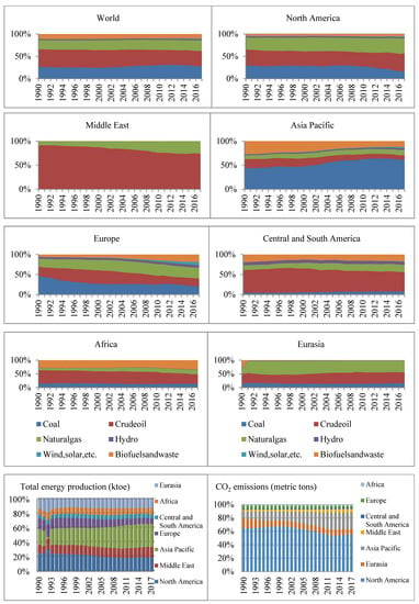
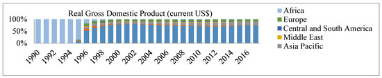
Figure 1.
Energy production, EG, and CO2 emissions.
Furthermore, Figure 1 also shows that North America and the Asia Pacific have the highest share of
energy production than other regions. At the same time, North America has the highest proportion of CO2 emissions, followed by the Asia Pacific. In this way, the figure presents the complete picture that those regions with a higher share of energy production face the highest proportion of CO2 emissions. Notably, North America follows the Asia Pacific in real GDP, which shows that these regions have a more significant proportion of CO2 emissions with more incomes. These developments raise various questions regarding energy production, environmental sustainability, and EG across
countries with different incomes.
Therefore, this study’s investigation is paramount; below, we explain it in more detail. To analyze the effect of EG and aggregate, as well as disaggregate energy production on CO2 emissions, we specified Equation (1), which is written as follows:
In Equation (1), the dependent variable is carbon emissions denoted by CO2, whereas the right-hand side of the equation shows independent variables. When all the variables are converted into natural logarithms, Equation (1) becomes:
where represents the intercept term, LN denotes the natural logarithm, and– indicate the elasticity of variables, whereas represents the error term.
3.2. Estimation Techniques
The procedure of estimation used in the study consisted of six main steps: (1) three tests as the Friedman CSD test, Pesaran CSD test, and the bias-adjusted LM test are used to test the cross-sectional dependency of the variables. (2) The slope homogeneity test is conducted. (3) Cross-sectional Im, Pesaran, and Shin (Pesaran CIPS) and the cross-sectional augmented Dickey–Fuller test (CADF) are conducted to test the stationary of all the variables. (4) The Westerlund panel cointegration test is applied to examine the cointegration relationship among all the variables of study in Section 3.2.4. (5) Three estimation techniques i.e., panel mean group (MG), augmented mean group (AMG), and common correlated effects mean group (CCEMG) are employed to estimate the long-term parameters. (6) The Dumitrescu–Hurlin (D–H) panel causality approach is used to investigate the causal relationship among the variables.
3.2.1. CSD Test
Since, in econometrics, CSD is an essential issue in panel data, we may estimate inconsistent and biased results by ignoring CSD [42,43,44]. Therefore, this study first tests the CSD using a semiparametric Friedman [45] CSD test, Pesaran [44] CSD test, and the bias-adjusted LM test before testing the stationarity properties of all the variables in all the regions.
Since we have fixed T and large N, use of the Pesaran CD test, Friedman test, and bias-adjusted LM test is appropriate. The Pesaran CD test is valid for large N and fixed T and may be expressed as:
In Equation (3), T shows the period, N indicates the sample size, and denotes the pairwise correlation coefficient gained from the OLS estimator for each cross-section i.
3.2.2. Slope Homogeneity Test
In the case of heterogeneous panel data, slope homogeneity may cause untrustworthy and misleading results [46]. To test the slope homogeneity phenomenon, Pesaran and Yamagata [47] established the method of Swamy [48]. In this study, we have a large N and fixed T, so we employ the slope homogeneity test presented by Pesaran and Yamagata [47], which is based on the homoscedasticity assumption framework for a fixed N relative to T.
3.2.3. Panel Unit Root Test
Since the issue of CSD is found across the countries in the panel data, first-generation panel unit root tests such as Levin, Lin and Chu (LLC); Im, Pesaran and Shin (IPS); Phillips–Perron; and Fisher ADF are not valid, because these tests do not allow CSD in the panel data. Therefore, Pesaran [49] developed second-generation unit root tests such as the cross-sectional augmented test (CIPS) and CADF, which allow CSD in the panel data to overcome the limitation of the first-generation unit root tests. The CADF can be calculated as follows:
In Equation (4), and represent the first difference of the individual series and cross-sectional averages of the lagged level, respectively.
We can compute CADF statistics by averaging the , and in the equation indicates the t-statistics.
3.2.4. Panel Cointegration Test
Westerlund [50] developed a test based on error–correction panel cointegration to examine the cointegration relationship among variables. Hence, conventional cointegration tests such as the Pedroni test developed by Pedroni [51] is not based on CSD, so it may create biased estimates. Since our data are cross-sectionally dependent, therefore, we employed Westerlund panel cointegration, which can be expressed as follows:
In Equation (8), represents the speed of adjustment of the system.
The Westerlund [50] cointegration test is based on the least squares results of that have the null hypothesis of no cointegration, and the group mean statistics of the Westerlund test are calculated as follows:
Furthermore, the panel statistics are obtained from the following formulas:
It may be concluded that cointegration exists in at least one cross-sectional unit of the panel when Gt and Ga reject the null hypothesis.
3.2.5. Panel Long-Term Estimates
After confirming the panel cointegration among the variables, we employed MG, AMG, and CCEMG for the long-term estimates of the study. Conventional panel regression methods could be inconsistent and biased in the presence of CSD [52,53,54,55]. The MG regression method was proposed by Pesaran and Smith [52], which allows error variances and their slope coefficients to change across the panels. This regression method obtains panel-specific slope coefficients through the OLS approach and then averages the specific coefficients of the panel. Further, the MG approach does not take into account information regarding common factors that can exist in the panel data. Eberhardt and Bond [56] and Eberhardt and Teal [57] introduced an AMG estimator that is highly robust regardless of slope heterogeneity and CSD. This approach uses the common dynamic effect parameter to capture the unobservable common factors. The first-difference OLS equation can specify the AMG estimator:
In Equation (13), denotes the specific coefficient of the panel, denotes the first difference operator, and indicates the parameters of the time dummies. The AMG is then derived from the averaged group-specific parameters across panels as described in the above Equation (13). In Equation (14), denotes the estimates of.
According to Bond and Eberhardt [58], the AMG approach provides consistent and unbiased estimates in a Monto Carlo simulation for different N and T. Therefore, we also employed the AMG approach to estimate the long-term parameters of our study. The CCEMG regression method which is also robust to slope homogeneity and CSD was developed by Pesaran [59].
In Equation (15), denotes the specific coefficient of the panel, represent the variables, indicates the unobserved common factor with heterogeneous factor, and and denote the error term and intercept, respectively.
3.2.6. Panel Causality Test
In examining the relationship among macroeconomic variables, testing causality among the variables is an important step that helps policymakers to make decisions regarding specific policies. Dumitrescu and Hurlin [60] introduced the D–H causality test for panel data. The D–H panel causality test is based on the Wald statistic of Granger [61], which allows CSD. Moreover, the null hypothesis and the alternative hypothesis of the D–H panel causality test can be written as follows in Equations (16) and (17):
4. Results and Discussion
4.1. The results of Slope Homogeneity and CSD Tests
We begin our analysis by testing the slope homogeneity and CSD across cross-sections in the panel. Particularly, we choose the classification of countries set by the IEA, which entails seven regions, and in each panel, we present seven diverse kinds of energy production.
Table 2 presents the results of the slope homogeneity and CSD test. The estimates of the Friedman cross-sectional test showed that the null hypothesis of no cross-sectional independence was rejected at 1% and 5% for all the panels, i.e., globally, as well as seven subpanels. Similarly, the bias-adjusted LM cross-sectional test estimates indicate that, for all the panels, the H0 of no cross-sectional independence was rejected at 1%, 5%, and 10%, except for subpanel Eurasia. For Eurasia, the H0 of no cross-sectional independence was not rejected. As long as the results of the Pesaran cross-sectional test showed that the H0 of no cross-sectional independence was not rejected for North America and Eurasia, the null hypothesis was rejected at 1% and 5% for other sub- and global panels. Furthermore, the estimates of both tests of slope homogeneity (Δadj, Δ) confirmed the absence of homogeneity, as these tests rejected the H0 of slope homogeneity.
Table 2.
Slope homogeneity analysis and CSD.
4.2. The results of Panel Unit Root Tests
After testing the slope homogeneity and CSD, we employed second-generation unit root tests (i.e., CIPS and CADF) to determine the integration and stationarity of variables. The unit root estimates are calculated by using the CIPS and CADF tests (Table 3). The estimated results of both tests showed that the H0 of the unit root is rejected at the first difference for most of the variables of the subpanels and the global panel. Further, the results also showed that only a few variables are stationary at the level. Accordingly, this order of integration allows us to employ error–correction-based panel cointegration tests to investigate whether there is a long-term equilibrium relation among the study’s variables.
Table 3.
Unit root results.
4.3. The results of the Panel Cointegration Test
Table 4 presents the estimates of the Westerlund panel cointegration test for all the subpanels and the global panel. The results of the Westerlund test showed that the null hypothesis of no long-term cointegration is rejected at 1% and 5% for all panels, indicating that a long-term relationship exists between CO2 and its determinants between 1990 and 2017. The existence of long-term cointegration among CO2 emissions, foreign trade, EG, total energy production, and its six subcomponents fulfills the primary aim of the study. Furthermore, it also enables us to examine the effect of these variables on CO2 emissions.
Table 4.
Westerlund panel cointegration results.
4.4. The Results of Panel Long-Term Estimators
After confirming the long-term panel cointegration among the variables, the next step is to explore the long-term estimates for the subpanels and global panels. In this section, we discuss the results of the MG, AMG, and CCEMG estimators. We notice that these three approaches provide us with similar, as well as dissimilar, estimates for all the subpanels, as well as the global panel. We begin with a discussion of estimates of MG, AMG, and CCEMG for the global panel and then investigate whether the results are similar for other subpanels. Here, the results of the global panel are given in the table and discussed afterward, but for other regions, only discussions have been made, and their relevant tables have not been fetched. These are available with the authors and can be sent to interested readers upon request. Table 5 presents the long-term estimates of the MG, AMG, and CCEMG specifications for checking the robustness of the global panel. According to the estimates of all three methods, some interesting facts are revealed. The results of all three estimators showed that the real trade is negative, as well as significant in most of the models. The results indicate that foreign trade is not fueling environmental pollution.
Table 5.
Long-term estimates of MG, AMG, and CCEMG for the global panel.
This study used real GDP as the proxy for economic growth. Findings indicate that it has a significantly positive impact on GHG emissions in the global panel analysis for all three econometric specifications. Over the past three decades, the rise in the EG level has caused climate change due to a surge in GHG. But an increase in real GDP cannot be the only variable to raise environmental degradation (ED) because ED is a complex issue. With this result, we find that it can significantly aggravate ED in the global panel. With carbon emissions raised by a rise in EG, there is an impact on other sectors such as health; hence, the need to access the impact of regulations and how emissions can be mitigated. Other factors affect the pollution level and act as moderating variables, such as trade and urbanization. Several relevant studies have already validated this paradox [16,17,18,19,20], thereby establishing mechanisms for attaining green growth and sustainable development.
Because relying on the conventional energy source for getting energy has a destructive impact on quality of the environment, focusing the RE sources are essential to attain sustainable EG, and this is in line with several previous studies [25,26,27]. The use of solar, wind, and hydropower energy has a significant adverse impact on carbon emissions. It means global economies are paying consideration to environmental sustainability and growing segments of their RE. All of RE source are not contributing at the same intensity. Results show that some of the variable magnitude is higher than the other, which shows their contribution in the total energy mix. Like hydropower is protent RE contributor in several nations of all regions, and they haven’t already reached gross theoretical capabilities. Concerning outcomes of biofuel and waste, hydro energy, and wind and solar energy, from AMG and CCEMG estimates, results do not report statistically significant effects on carbon emissions.
Non-RE source variables, i.e., CO, NG, and COAL, along with TOP are positive and highly significant, implying that more non-RE sources increases countries’ emission level. All three selected econometric specifications’ gave unique outcomes, except for lnCO in AMG specification, which showed an insignificant effect on dependent variables. Part of what we find in this outcome is that in global panel economies, non-RE sources have a significant negative association with environmental quality. Unlike the RE, an increase in TEP, CO, NG, and COAL will raise ED and adversely impact the efforts for sustainable development. In particular, aside from the MG estimates, advancing renewable energy production sources like biofuels and waste, wind and solar, and hydro energy are subcomponents of total energy production, significantly increasing environmental quality. These estimates strengthen our view that RE sources (i.e., BW, H, WS, etc.) lower the environmental pollution.
Estimates of MG, AMG, and CCEMG for North America: Results showed that real trade has significantly adverse effects on regional emissions. At the same time, economic growth showed a positive and statistically significant impact on emissions. An exceptional outcome was observed from the CCEMG estimator, which showed that growth is adversely impacting the environmental quality. Another study by Dong et al. [20] for North America found a similar association between EG and ED. Results reported that RE variables, i.e., hydro energy, WS, and BW have significant adverse effects on the dependent variable and strengthen the view about the negative impact of RE sources on environmental pollution (for MG and AMG econometric specifications).
Conversely, CCEMG estimates for WS and BW do not appear to affect emissions. Results conclude that it is not necessary that RE energy is contributing positively to the environment in any case for any region of the world. On a final note, the results of all estimators for no-RE such as coal, crude oil, and natural gas, have a significantly positive contribution to ED. Although RE is supporting North America to attain sustainable development, but till now, it has not got a level where it can substantially influence ED.
Estimates of MG, AMG, and CCEMG for the Middle East: Aside from AMG estimates, real foreign trade (RT) has a significant adverse effect on the environment. The same was observed for the global panel. Conversely, the estimates of AMG showed that the variable RT has no significant effect on emissions in most of the models. Importantly, real growth has a significantly positive impact on the dependent variable. It is not surprising that growth significantly negatively affects the environment considering the EKC hypothesis. Prominent among other estimates is that non-RE variables such as CO, TEP, and natural gas seem to exert a positive effect on the environment, except the coal energy.
Coal energy production does not significantly impact this region’s environmental pollution. All estimators provide dissimilar results, such as hydroenergy, biofuel, and waste energy. According to the estimates of MG, hydroenergy has a significantly positive impact on the environment, but BW and WS variables do not exert a significant effect on emissions. In parallel, the results of AMG showed that biofuel and waste energy (BW) are decreasing environmental degradation. In contrast, the variable wind and solar energy production appear to have a positive effect on emissions as long as the AMG estimator does not provide significant results for hydroenergy. Finally, aside from the biofuel and waste energy source, the CCEMG estimator provides us with significant estimates for the WS and hydroenergy variables. Turning to the magnitude, there is less effect of these variables on the dependent variable than other non-RE sources such as coal, crude oil, and natural gas. Regarding variables relating to RE sources, such as biofuels and waste, hydro and wind and solar, etc., these estimates indicate that the results are diversified in this region.
Estimates of MG, AMG, and CCEMG for the Asia Pacific: Unlike the cases of the global panel and other subpanels discussed above, real foreign trade is significantly reducing the environmental pollution in the Asia Pacific region (according to MG specification for most of the selected models). But these findings contradict the outcomes of the latest study on 17 Asia Pacific economies by Rahman and Alam (2022), which found an inverse association between environmental quality and RT variables. Contrarily the other two econometric specification (AMG and CCEMG) estimates showed that real growth positively contributes to pollution.
The results of biofuels and waste energy production (AMG estimates) and hydroenergy production (CCEMG estimates) proved that these significantly reduce ED in the region. These results validated the study by Bhattacharya et al. [7] conducted on thirty-eighty nations for 1991-2012 panel data, who reported that the use of non-exhaustible energy positively contributes to promoting EG and helps in controlling ED. However, the other results for other RE sources for three specifications indicated that the production of RE increases environmental pollution in this region. On the other hand non-RE variables (natural gas, crude oil, coal) showed positive association with GHG escalation as was found for other subpanels discussed above. All of RE and no-RE variables’ coefficients were statistically significant at one of five percent except for coal energy (COAL) and hydroenergy (H).
Estimates of MG, AMG, and CCEMG for Europe: The estimated results of MG, AMG and CCEMG were not similar for variable lnRT in case of European region. But for most cases, the estimated coefficient of trade was significantly decreasing ED. Turning to lnRGDP, findings claimed its positive and statistically significant impact on environmental deterioration. This result also strengthens our view that growth significantly increases environmental pollution in this region. Furthermore, concerning variables biofuels and waste energy (BW), hydroenergy (H), and Wind and Solar energy (WS), all analyses provide statistically significant negative coefficients. It shows that energy production from these sources help in controlling carbon emission and contribute to a sustainable environment. But in parallel, wind and solar energy variables behaved differently and showed a significantly positive correlation with ED.
Regarding non-RE source variables, all variables such as natural gas energy (NG), crude oil (CO), and coal showed similar findings as were quantified for most of the above panels. These results were according to the expectations. While for CCEMG specification, results did not provide significant coefficient values for CO and NG. Overall we can conclude that the production of energy from coal, natural gas, and crude oil sources is enhancing ED in Europe overtime. Similar findings were reported by Przychodzen and Przychodzen [25] for a 1990-2014 panel data study on renewable electricity for European nations.
Estimates of MG, AMG, and CCEMG for Central and South America: Similarly to previous regions, the estimated results of all approaches displayed that the variables of foreign trade and real growth (RGDP) have significant magnitudes. The value of real growth is closely linked to environmental pollution and positively impacts it. In parallel, the variable RT contributes to a healthy environment. We notice that these results imply that carbon emission is inversely affected by foreign trade while positively affected by growth in the region. Further, concerning energy variables, the MG estimator mostly provides insignificant coefficients, except for hydroenergy and natural gas.
Conversely, AMG and CCEMG estimators indicate that, except hydroenergy and WS, all other variables hurt the environment; these energy sources reduce environmental degradation. Most importantly, the CCEMG provides negative coefficient values that indicate these contribute to a sustainable environment. These findings validate the research study related to 128 economies by Dong et al. [20], who claimed that EG and population increase and RE declines CO2 emission in all selected regions, including South America. On the other hand, NG, CO and COAL variables have significantly positive coefficient values for both techniques.
Estimates of MG, AMG, and CCEMG for Africa: For the African region, all three econometrics methods showed that coefficient values related to real trade (lnRT) and RGDP as a proxy of EG have negative and positive signs, respectively. For both variables, all models own statistically significant worth for three specifications (except RT in CCEMG for two models). These estimates indicate that foreign trade positively impacts environmental quality while EG positively contributes to environmental pollution. All the estimators provide similar findings for TEP, BW, NG, and COAL, but different results for the remaining three energy source variables. The estimates of former variables showed that all the sources of energy production are positively linked with environmental deterioration in the form of carbon dioxide discharge. Surprisingly, the MG estimator does not provide significant results for RE variables i.e., hydroenergy, wind, and solar energy and the same was observed for another sub-panel regarding MG estimator. In parallel, AMG estimated that crude oil reduces carbon emissions. Similarly, the outcomes of CCEMG showed that wind and solar energy production has a negative coefficient value, which means it plays a positive role in a sustainable environment.
Estimates of MG, AMG, and CCEMG for Eurasia: Variables of RT and RGDP appear to have statistically significant results in all the regions. Apparently, for Eurasia, these variables have a significant impact on environmental degradation. All types of energy production have a significantly positive effect on pollution. Finally, the CCEMG estimator does not provide a significant magnitude of total energy production.
Summarizing these findings, we can draw some suitable conclusions. To begin with, it is quite essential to note that all three econometric specifications provide significant responses to all the variables of the study for all the regions. Each estimator provides different findings of variables (e.g., BW, WS, and H) for each region. In turn, real growth indeed increases environmental pollution in all regions. The results show that foreign trade lowers environmental pollution in a global panel and in other subpanels.
Furthermore, it is more surprising that the coal energy source is losing its importance in the Middle East and Asia Pacific. This response might be due to the recent trend in developing and developed countries to produce natural gas and oil instead of coal [62,63,64]. At the same time, all the estimators showed that crude oil and natural gas reflect positive responses toward carbon emissions in selected regions. In this way, these energy production sources are getting more importance as an energy source rather than coal for selected regions. In particular, it should be noted that the innovation in energy production sources which are subcomponents of total energy production such as BW, WS, and hydroenergy have a significant positive effect on environmental degradation in Global panel, Middle East, Central and South America, the Asia Pacific, Africa, and Eurasia, though their effect is much lower than non-RE such as coal, crude oil, and natural gas. These variables mostly contribute to carbon emissions reduction for North America and Europe. These estimates are consistent with the findings of Ocal and Aslan [65], who stressed that RE sources are expensive, especially for developing countries, and therefore, these countries cannot adopt such expensive methods for energy production.
Additionally, these estimates question the performance of government policies of different countries regarding the production of RE as a substitute for non-RE for the promotion of EG. These policies include establishing markets for RE certificates and tax credits for the production of RE, as well as various reimbursements for installing projects for the production of RE [66,67]. Arguably, producing energy from RE sources is important for environmental sustainability.
Likewise, in light of our estimates, those countries should focus on producing energy from renewable sources rather than nonrenewable sources to sustain the current growth pace. Dincer [68] examined the link between sustainable development and RE and argued that sustainable development should be anticipated upon the RE supply. Moreover, additional research and development might assess actual environmental benefits and EG more precisely. In many respects, our results navigate the discussion toward the newsworthy issue of whether economies should levy limits on EG. Some authors argued that overproduction might deploy fresh water resources, over-exploitation of productive land, and higher greenhouse gas emissions (see refs. [69,70,71] for detail). In this way, the current generations should carefully use natural resources for sustainable growth. Thus, the discussion is closely linked to the rebound effect argument, which indicates that even more energy-saving and efficient technologies are not necessary for environmental concerns [72,73,74,75]. This argument strengthens our findings for the RE variables such as hydroenergy, WS, and BW. In the next section, we report each panel’s estimates of D–H Granger causality to get a clear theme regarding the impact of EG, energy production, and its subcomponents in the environment.
4.5. The Outcomes of the Panel Causality Test
The tables of D–H Granger causality findings are available with the authors and can be fetched on request. The causality test findings revealed some interesting patterns. Firstly, there is two-way causality between EG and emissions in the global panel, Africa, Central, and South America, whereas, in all other panels apart from the Asia Pacific and Eurasia, and there is no evidence of causality between EG and CO2 emissions. Additionally, EG does Granger cause emissions in Eurasia at a 5% level of statistical significance. Thus, the findings showed that the EKC hypothesis is verified in all the panels aside from the Middle East, Europe, and North America. Secondly, two-way causality between foreign trade and CO2 emissions exists only for Europe’s region, while we found no evidence of causality in North America, Eurasia, and the Middle East. In addition, foreign trade is Granger-linked, caused by carbon emissions in the global panel, Africa, and Central and South America. Conversely, in the Asia Pacific, foreign trade does Granger cause to CO2 emissions.
Thirdly, we found no evidence of causality between foreign trade and EG in North America, Africa, and Eurasia, but in parallel, there is two-way causality between EG and foreign trade in the Asia Pacific and Central and South America. EG has a link with foreign trade only in the global panel and the Middle East, while in Europe, EG has link with foreign trade. Fourthly, bidirectional causality between total energy production and emissions is found only in Europe. We noticed that, apart from Africa and Central and South America, there is no causality from the total energy production to the environment. Fifthly, we found two-way causality between the total energy production and EG in Central and South America, and thus, we noticed that the feedback hypothesis is verified only in Central and South America. Conversely, we found no causal relationship between EG and total energy production in North America, Middle East, and Asia Pacific that verified the neutrality hypothesis in these panels.
Aside from Eurasia, there is a unidirectional relationship from EG to total energy production in the global panel, Europe, and Africa, and a further conservation hypothesis was also verified in these panels. In the same way, the growth hypothesis is also verified in a global panel and Africa, as EG does Granger cause total energy production in both panels. Additionally, there is no evidence of a causal relationship between foreign trade and total energy production in North America, Europe, Africa, and Eurasia. In the Middle East, we found bidirectional causality between total energy production and foreign trade, but total energy production does Granger cause foreign trade in the global panel and Central and South America. On the other hand, unidirectional causality running from foreign trade to total energy production exists only in the Asia Pacific.
Furthermore, we explain above that total energy production does Granger cause to EG, but this is not for all panels, so the estimates fail to consider specific differences regarding energy production among various classifications of countries. To this end, we continue our findings with subcomponents of energy to check the effects. In turn, we found bidirectional causality between coal energy production and CO2 emissions, crude oil and CO2 emissions, biofuel wastes, and CO2 emissions in the Middle East, global panel, Europe, and Africa, respectively. On the other hand, we notice that coal energy production appears to cause EG and foreign trade in North America and the Asia Pacific and in all the panels apart from North America, Europe, and Africa, respectively. Natural gas does Granger cause to CO2 emissions in all regions apart from the global panel, Middle East, and Africa, as well as the Granger link to EG in the global panel, Middle East, Europe, and the Asia Pacific. Natural gas showed link with foreign trade in Asia and Africa. It is not surprising that crude oil causes CO2 emissions in the global panel, Middle East, Africa, and Eurasia. However, it cause EG in about all the panels except from North America, the Asia Pacific, and Central and South America.
Additionally, we found evidence of unidirectional causality running from crude oil and foreign trade in the Middle East, Eurasia, Europe, and Central and South America. We found a bidirectional causal relationship between biofuels and waste and CO2 emissions in Europe and Africa but a unidirectional relationship between CO2 emissions toward biofuels and waste in North America only. Similarly, foreign trade is also caused by biofuels and waste in the global panel, Europe, Africa, and Eurasia. Surprisingly, we found no evidence of causality running from wind and solar energy production toward CO2 emissions in none of the panels. Nonetheless, if we concentrate on hydropower energy production, it appears to cause CO2 emissions in the global panel, Middle East, Europe, and Africa, but at the same time, CO2 emissions Granger cause hydropower energy production only in the Asia Pacific panel. Turning to hydropower and EG, we notice that hydropower energy production causes EG only in the Asia Pacific, Europe, and Central and South America. However, in parallel, no single evidence of causality runs from EG to hydropower energy production in any of the panels. Unidirectional causality runs from hydropower and foreign trade only in the Asia Pacific and Central and South America. Moreover, we notice that all types of energy production do not Granger cause CO2 emissions in the global panel. Similarly, in North America, only natural gas, biofuels, and waste Granger cause CO2 emissions. Finally, we see that all types of energy production do not Granger cause CO2 emissions in none of the panels.
5. Summary and Concluding Remarks
This article examined the intricate linkages among carbon emissions, EG, and energy production for 99 countries that are classified into seven distinct regions by IEA. To do this, the study started its empirical analysis by determining if the data have any CSD. We conducted the CIPS and CADF second-generation unit root tests after identifying CSD in the series, and all variables were found to be first-order stationary. Then, to ascertain the long-term cointegration among the study’s variables, we employed the Westerlund cointegration technique. Following the confirmation of cointegration, the MG, AMG, CCEMG regression techniques, and D–H panel causality tests were used to examine the relationship between the variables.
The results of all the approaches showed that biofuels and waste energy production, hydroenergy production, and wind and solar and other energy production sources are decreasing CO2 emissions. Similarly, foreign trade alleviates CO2 emissions. However, GDP growth, total energy production, crude oil energy production, coal energy production, and natural gas energy production exacerbate increased environmental degradation and, thus, contribute to environmental deterioration. Meanwhile, coal energy production has an insignificant impact on CO2 emissions in the Middle East and Asia Pacific regions. Further, each estimator provides dissimilar estimates in each region for hydroenergy production, biofuels, and waste, as well as wind and solar energy production.
The following recommendation and related policy consequences are suggested. First, as, we found that GDP growth increases GHG emissions in all the regions of the world, the EG strategies of all areas should be in line with their environmental development agendas to raise EG rates without increasing emissions connected to energy production. Furthermore, our findings showed that energy production from non-RE sources, including coal, crude oil, and natural gas, increase environmental degradation. In contrast, RE sources such as biofuels and waste, hydro and wind, and solar energy production decrease environmental degradation in most regions. However, we cannot report any strong argument that the production of energy from RE sources is more efficient, environmentally sustainable, and able to promote the growth of some regions. The reason may be the cost of producing RE and the significant lack of interest in RE. The underutilization of their RE potential might be another factor. Therefore, these regions should focus on increasing or enhancing their energy production mix, including RE production. By increasing their production of RE in the upcoming years, all regions would strengthen their economies and environmental conditions.
To further a low-carbon economy with sustainable EG, all the regions should develop policies to prevent the production of fossil fuels such as coal, crude oil, and natural gas and encourage energy conservation and new energy sources, particularly wind, solar, hydro, biofuels, and waste energy projects. Additionally, by facilitating the transition to RE across all the regions, investment in the development of RE technology can assist further in lowering the region’s energy-related emission levels. The current research mainly focuses on a few control variables, so future studies may utilize additional control factors to analyze this connection and to promote studies of this topic among similar income groups.
Author Contributions
Conceptualization, S.A.A.N.; Formal analysis, S.A.A.N., B.H. and M.A.U.R.T.; Methodology, B.H.; Writing—original draft, A.A.S.; Writing—review & editing, M.U. All authors have read and agreed to the published version of the manuscript.
Funding
This research received no external funding.
Data Availability Statement
Data can be provided on serious request.
Acknowledgments
The authors are very grateful to all those who provided help during this research.
Conflicts of Interest
The authors declared no potential conflict of interest.
Appendix A
Table A1.
List of countries.
Table A1.
List of countries.
| Sub Panel | Countries |
| Middle East (9 countries) | Islamic Republic of Iran, Saudi Arabia, United Arab Emirates, Iraq, Qatar, Kuwait, Oman, Jordan, Syria. |
| Africa (18 countries) | Nigeria, South Africa, Egypt, Algeria, Congo, Morocco, Tanzania, Angola, Libya, Zambia, Tunisia, Zimbabwe, Cote d’Ivoire, Cameroon, Ghana, Gabon, Senegal, Botswana. |
| North America (3 countries) | United States, Canada, Mexico. |
| Central and South America (15 countries) | Brazil, Venezuela, Colombia, Chile, Peru, Trinidad and Tobago, Ecuador, Guatemala, Bolivia, Dominican Republic, Uruguay, Costa Rica, El Salvador, Nicaragua, Jamaica. |
| Asia Pacific (16 countries) | People’s Republic of China, India, Japan, Indonesia, Thailand, Australia, Pakistan, Malaysia, Viet Nam, Philippines, Bangladesh, Myanmar, New Zealand, Nepal, Sri Lanka, Mongolia. |
| Eurasia (6 countries) | Russian Federation, Kazakhstan, Georgia, Kyrgyzstan, Azerbaijan, Tajikistan. |
| Europe (32 countries) | Germany, France, United Kingdom, Italy, Turkey, Spain, Poland, Ukraine, Netherlands, Belgium, Sweden, Czech Republic, Austria, Romania, Finland, Norway, Hungary, Switzerland, Greece, Israel, Portugal, Bulgaria, Slovak Republic, Denmark, Serbia, Ireland, Croatia, Lithuania, Slovenia, Bosnia and Herzegovina, Albania, North Macedonia, Latvia. |
| Global Panel (99 countries) | Germany, France, United Kingdom, Italy, Turkey, Spain, Poland, Ukraine, Netherlands, Belgium, Sweden, Czech Republic, Austria, Romania, Finland, Norway, Hungary, Switzerland, Greece, Israel, Portugal, Bulgaria, Slovak Republic, Denmark, Serbia, Ireland, Croatia, Lithuania, Slovenia, Bosnia and Herzegovina, Albania, North Macedonia, Latvia, People’s Republic of China, India, Japan, Indonesia, Thailand, Australia, Pakistan, Malaysia, Viet Nam, Philippines, Bangladesh, Myanmar, New Zealand, Nepal, Sri Lanka, Mongolia, Russian Federation, Kazakhstan, Georgia, Kyrgyzstan, Azerbaijan, Tajikistan, Brazil, Venezuela, Colombia, Chile, Peru, Trinidad and Tobago, Ecuador, Guatemala, Bolivia, Dominican Republic, Uruguay, Costa Rica, El Salvador, Nicaragua, Jamaica, United States, Canada, Mexico, United States, Canada, Mexico, Nigeria, South Africa, Egypt, Algeria, Congo, Morocco, Tanzania, Angola, Libya, Zambia, Tunisia, Zimbabwe, Cote d’Ivoire, Cameroon, Ghana, Gabon, Senegal, Botswana. |
References
- Jardón, A.; Kuik, O.; Tol, R.S. Economic growth and carbon dioxide emissions: An analysis of Latin America and the Caribbean. Atmósfera 2017, 30, 87–100. [Google Scholar] [CrossRef]
- Tol, R.S. The economic effects of climate change. J. Econ. Perspect. 2009, 23, 29–51. [Google Scholar] [CrossRef]
- Owusu, P.A.; Asumadu-Sarkodie, S. A review of renewable energy sources, sustainability issues and climate change mitigation. Cogent. Eng. 2016, 3, 1167990. [Google Scholar] [CrossRef]
- Chen, Y.; Wang, Z.; Zhong, Z. CO2 emissions, economic growth, renewable and non-renewable energy production and foreign trade in China. Renew. Energy 2019, 131, 208–216. [Google Scholar] [CrossRef]
- Bilgili, F.; Koçak, E.; Bulut, Ü. The dynamic impact of renewable energy consumption on CO2 emissions: A revisited Environmental Kuznets Curve approach. Renew. Sustain. Energy Rev. 2016, 54, 838–845. [Google Scholar] [CrossRef]
- Goh, T.; Ang, B.W. Quantifying CO2 emission reductions from renewables and nuclear energy–some paradoxes. Energy Policy 2018, 113, 651–662. [Google Scholar] [CrossRef]
- Bhattacharya, M.; Churchill, S.A.; Paramati, S.R. The dynamic impact of renewable energy and institutions on economic output and CO2 emissions across regions. Renew. Energy 2017, 111, 157–167. [Google Scholar] [CrossRef]
- Dong, K.; Sun, R.; Hochman, G. Do natural gas and renewable energy consumption lead to less CO2 emission? Empirical evidence from a panel of BRICS countries. Energy 2017, 141, 1466–1478. [Google Scholar] [CrossRef]
- United Nations Industrial Development Organization. Clean Energy Access for Production Use. 2019. Available online: https://www.unido.org/our-focus/safeguarding-environment/clean-energy-access-productive-use/renewable-energy (accessed on 1 June 2022).
- Wang, L.; Tao, Z. Dynamic relationship among consumption of renewable energy, economic growth and carbon emission in China. Technol. Econ. 2013, 32, 99–104. [Google Scholar]
- Wang, Z.; Feng, C. Sources of production inefficiency and productivity growth in China: A global data envelopment analysis. Energy Econ. 2015, 49, 380–389. [Google Scholar] [CrossRef]
- Lin, B.; Moubarak, M. Renewable energy consumption–economic growth nexus for China. Renew. Sustain. Energy Rev. 2014, 40, 111–117. [Google Scholar] [CrossRef]
- Long, X.; Naminse, E.Y.; Du, J.; Zhuang, J. Nonrenewable energy, renewable energy, carbon dioxide emissions and economic growth in China from 1952 to 2012. Renew. Sustain. Energy Rev. 2015, 52, 680–688. [Google Scholar] [CrossRef]
- Jalil, A.; Mahmud, S.F. Environment Kuznets curve for CO2 emissions: A cointegration analysis for China. Energy Policy 2009, 37, 5167–5172. [Google Scholar] [CrossRef]
- Rahman, Z.U.; Khattak, S.I.; Ahmad, M.; Khan, A. A disaggregated-level analysis of the relationship among energy production, energy consumption and economic growth: Evidence from China. Energy 2020, 194, 116836. [Google Scholar] [CrossRef]
- Antonakakis, N.; Chatziantoniou, I.; Filis, G. Energy consumption, CO2 emissions, and economic growth: An ethical dilemma. Renew. Sustain. Energy Rev. 2017, 68, 808–824. [Google Scholar] [CrossRef]
- Jebli, M.B.; Farhani, S.; Guesmi, K. Renewable energy, CO2 emissions and value added: Empirical evidence from countries with different income levels. Struct. Change Econ. Dyn. 2020, 53, 402–410. [Google Scholar] [CrossRef]
- Rahman 2020, M.M.; Velayutham, E. Renewable and non-renewable energy consumption-economic growth nexus: New evidence from South Asia. Renew. Energy 2020, 147, 399–408. [Google Scholar] [CrossRef]
- Maji, I.K.; Sulaiman, C.; Abdul-Rahim, A.S. Renewable energy consumption and economic growth nexus: A fresh evidence from West Africa. Energy Rep. 2019, 5, 384–392. [Google Scholar] [CrossRef]
- Dong, K.; Hochman, G.; Zhang, Y.; Sun, R.; Li, H.; Liao, H. CO2 emissions, economic and population growth, and renewable energy: Empirical evidence across regions. Energy Econ. 2018, 75, 180–192. [Google Scholar] [CrossRef]
- Le, H.P.; Bao, H.H.G. Renewable and nonrenewable energy consumption, government expenditure, institution quality, financial development, trade openness, and sustainable development in Latin America and Caribbean emerging Market and developing economies. Int. J. Energy Econ. Policy 2020, 10, 242. [Google Scholar] [CrossRef]
- Sarkodie, S.A.; Strezov, V. Assessment of contribution of Australia’s energy production to CO2 emissions and environmental degradation using statistical dynamic approach. Sci. Total Environ. 2018, 639, 888–899. [Google Scholar] [CrossRef] [PubMed]
- Sarkodie, S.A.; Strezov, V.; Weldekidan, H.; Asamoah, E.F.; Owusu, P.A.; Doyi, I.N.Y. Environmental sustainability assessment using dynamic autoregressive-distributed lag simulations—nexus between greenhouse gas emissions, biomass energy, food and economic growth. Sci. Total Environ. 2019, 668, 318–332. [Google Scholar] [CrossRef] [PubMed]
- Ahmad, N.; Du, L. Effects of energy production and CO2 emissions on economic growth in Iran: ARDL approach. Energy 2017, 123, 521–537. [Google Scholar] [CrossRef]
- Przychodzen, W.; Przychodzen, J. Determinants of renewable energy production in transition economies: A panel data approach. Energy 2020, 191, 116583. [Google Scholar] [CrossRef]
- Bento, J.P.C.; Moutinho, V. CO2 emissions, non-renewable and renewable electricity production, economic growth, and international trade in Italy. Renew. Sustain. Energy Rev. 2016, 55, 142–155. [Google Scholar] [CrossRef]
- Dabachi, U.M.; Mahmood, S.; Ahmad, A.U.; Ismail, S.; Farouq, I.S.; Jakada, A.H.; Kabiru, K. Energy Consumption, Energy Price, Energy Intensity Environmental Degradation, and Economic Growth Nexus in African OPEC Countries: Evidence from Simultaneous Equations Models. J. Environ. Treat. Tech. 2020, 8, 403–409. [Google Scholar]
- Le, T.H.; Chang, Y.; Park, D. Renewable and nonrenewable energy consumption, economic growth, and emissions: International evidence. Energy J. 2020, 41, 73–92. [Google Scholar] [CrossRef]
- Begum, R.A.; Sohag, K.; Abdullah, S.M.S.; Jaafar, M. CO2 emissions, energy consumption, economic and population growth in Malaysia. Renew. Sustain. Energy Rev. 2015, 41, 594–601. [Google Scholar] [CrossRef]
- Zafar, M.W.; Shahbaz, M.; Hou, F.; Sinha, A. From nonrenewable to renewable energy and its impact on economic growth: The role of research & development expenditures in Asia-Pacific Economic Cooperation countries. J. Clean. Prod. 2019, 212, 1166–1178. [Google Scholar]
- Wang, Z.; Bui, Q.; Zhang, B. The relationship between biomass energy consumption and human development: Empirical evidence from BRICS countries. Energy 2020, 194, 116906. [Google Scholar] [CrossRef]
- Sharif, A.; Mishra, S.; Sinha, A.; Jiao, Z.; Shahbaz, M.; Afshan, S. The renewable energy consumption-environmental degradation nexus in Top-10 polluted countries: Fresh insights from quantile-on-quantile regression approach. Renew. Energy 2020, 150, 670–690. [Google Scholar] [CrossRef]
- Raza, S.A.; Shah, N.; Sharif, A. Time frequency relationship between energy consumption, economic growth and environmental degradation in the United States: Evidence from transportation sector. Energy 2019, 173, 706–720. [Google Scholar] [CrossRef]
- Mutascu, M.; Sokic, A. Trade Openness-CO2 Emissions Nexus: A Wavelet Evidence from EU. Environ. Modeling Assess. 2020, 25, 411–428. [Google Scholar] [CrossRef]
- Jammazi, R.; Aloui, C. RETRACTED: On the interplay between energy consumption, economic growth and CO2 emission nexus in the GCC countries: A comparative analysis through wavelet approaches. Renew. Sustain. Energy Rev. 2015, 51, 1737–1751. [Google Scholar] [CrossRef]
- Menegaki, A.N.; Tsagarakis, K.P. Rich enough to go renewable 2015, but too early to leave fossil energy? Renew. Sustain. Energy Rev. 2015, 41, 1465–1477. [Google Scholar] [CrossRef]
- Ajmi, A.N.; El Montasser, G.; Nguyen, D.K. Testing the relationships between energy consumption and income in G7 countries with nonlinear causality tests. Econ. Model. 2013, 35, 126–133. [Google Scholar] [CrossRef]
- Kula, F.E.R.İ.T. The long-run relationship between renewable electricity consumption and GDP: Evidence from panel data. Energy Sources Part B Econ. Plan. Policy 2014, 9, 156–160. [Google Scholar] [CrossRef]
- Apergis, N.; Payne, J.E.; Menyah, K.; Wolde-Rufael, Y. On the causal dynamics between emissions, nuclear energy, renewable energy, and economic growth. Ecol. Econ. 2010, 69, 2255–2260. [Google Scholar] [CrossRef]
- Salahuddin, M.; Gow, J.; Ozturk, I. Is the long-run relationship between economic growth, electricity consumption, carbon dioxide emissions and financial development in Gulf Cooperation Council Countries robust? Renew. Sustain. Energy Rev. 2015, 51, 317–326. [Google Scholar] [CrossRef]
- Cowan, W.N.; Chang, T.; Inglesi-Lotz, R.; Gupta, R. The nexus of electricity consumption, economic growth and CO2 emissions in the BRICS countries. Energy Policy 2014, 66, 359–368. [Google Scholar] [CrossRef]
- Bilgili, F.; Ulucak, R. Is there deterministic, stochastic, and/or club convergence in ecological footprint indicator among G20 countries? Environ. Sci. Pollut. Res. 2018, 25, 35404–35419. [Google Scholar] [CrossRef] [PubMed]
- Grossman, G.M.; Krueger, A.B. Economic growth and the environment. Q. J. Econ. 1995, 110, 353–377. [Google Scholar] [CrossRef]
- Pesaran, H.M. General Diagnostic Tests for Cross-Sectional Dependence in Panels; Cambridge Working Papers in Economics; University of Cambridge: Cambridge, UK, 2004; p. 435. [Google Scholar]
- Friedman, M. The use of ranks to avoid the assumption of normality implicit in the analysis of variance. J. Am. Stat. Assoc. 1937, 32, 675–701. [Google Scholar] [CrossRef]
- Breitung, J. A parametric approach to the estimation of cointegration vectors in panel data. Econom. Rev. 2005, 24, 151–173. [Google Scholar] [CrossRef]
- Pesaran, M.H.; Yamagata, T. Testing slope homogeneity in large panels. J. Econom. 2008, 142, 50–93. [Google Scholar] [CrossRef]
- Swamy, P.A. Efficient inference in a random coefficient regression model. Econom. J. Econom. Soc. 1970, 38, 311–323. [Google Scholar] [CrossRef]
- Pesaran, M.H. A simple panel unit root test in the presence of cross-section dependence. J. Appl. Econom. 2007, 22, 265–312. [Google Scholar] [CrossRef]
- Westerlund, J. Testing for error correction in panel data. Oxf. Bull. Econ. Stat. 2007, 69, 709–748. [Google Scholar] [CrossRef]
- Pedroni, P. Purchasing power parity tests in cointegrated panels. Rev. Econ. Stat. 2001, 83, 727–731. [Google Scholar] [CrossRef]
- Pesaran, M.H.; Smith, R. Estimating long-run relationships from dynamic heterogeneous panels. J. Econom. 1995, 68, 79–113. [Google Scholar] [CrossRef]
- Phillips, P.C.; Sul, D. Dynamic panel estimation and homogeneity testing under cross section dependence. Econom. J. 2003, 6, 217–259. [Google Scholar] [CrossRef]
- Sarafidis, V.; Robertson, D. On the impact of error cross-sectional dependence in short dynamic panel estimation. Econom. J. 2009, 12, 62–81. [Google Scholar] [CrossRef]
- Paramati, S.R.; Mo, D.; Gupta, R. The effects of stock market growth and renewable energy use on CO2 emissions: Evidence from G20 countries. Energy Econ. 2017, 66, 360–371. [Google Scholar] [CrossRef]
- Eberhardt, M.; Bond, S. Cross-Section Dependence in Nonstationary Panel Models: A Novel Estimator; University Library of Munich: Munich, Germany, 2009. [Google Scholar]
- Eberhardt, M.; Teal, F. Productivity Analysis in Global Manufacturing Production (Discussion Paper 515); Department of Economics, University of Oxford: Oxford, UK, 2010. [Google Scholar]
- Bond, S.; Eberhardt, M. Accounting for Unobserved Heterogeneity in Panel Time Series Models; University of Oxford: Oxford, UK, 2013. [Google Scholar]
- Pesaran 2013, M.H. Estimation and inference in large heterogeneous panels with a multifactor error structure. Econometrica 2006, 74, 967–1012. [Google Scholar] [CrossRef]
- Dumitrescu, E.I.; Hurlin, C. Testing for Granger non-causality in heterogeneous panels. Econ. Model. 2012, 29, 1450–1460. [Google Scholar] [CrossRef]
- Granger, C.W. Investigating causal relations by econometric models and cross-spectral methods. Econom. J. Econom. Soc. 1969, 37, 424–438. [Google Scholar] [CrossRef]
- Yang, C.J.; Xuan, X.; Jackson, R.B. China’s coal price disturbances: Observations, explanations, and implications for global energy economies. Energy Policy 2012, 51, 720–727. [Google Scholar] [CrossRef]
- Howarth, R.W.; Ingraffea, A.; Engelder, T. Natural gas: Should fracking stop? Nature 2011, 477, 271–275. [Google Scholar] [CrossRef]
- Chen, S.; Golley, J. 2014. ‘Green’productivity growth in China’s industrial economy. Energy Econ. 2011, 44, 89–98. [Google Scholar] [CrossRef]
- Ocal, O.; Aslan, A. Renewable energy consumption–economic growth nexus in Turkey. Renew. Sustain. Energy Rev. 2013, 28, 494–499. [Google Scholar] [CrossRef]
- Apergis, N.; Payne, J.E. Renewable and non-renewable energy consumption-growth nexus: Evidence from a panel error correction model. Energy Econ. 2012, 34, 733–738. [Google Scholar] [CrossRef]
- Apergis, N.; Payne, J.E. Renewable energy, output, CO2 emissions, and fossil fuel prices in Central America: Evidence from a nonlinear panel smooth transition vector error correction model. Energy Econ. 2014, 42, 226–232. [Google Scholar] [CrossRef]
- Dincer, I. Renewable energy and sustainable development: A crucial review. Renew. Sustain. Energy Rev. 2000, 4, 157–175. [Google Scholar] [CrossRef]
- Galli, A.; Wiedmann, T.; Ercin, E.; Knoblauch, D.; Ewing, B.; Giljum, S. Integrating ecological, carbon and water footprint into a “footprint family” of indicators: Definition and role in tracking human pressure on the planet. Ecol. Indic. 2012, 16, 100–112. [Google Scholar]
- Weinzettel, J.; Steen-Olsen, K.; Hertwich, E.G.; Borucke, M.; Galli, A. Ecological footprint of nations: Comparison of process analysis, and standard and hybrid multiregional input–output analysis. Ecol. Econ. 2014, 101, 115–126. [Google Scholar] [CrossRef]
- Hoekstra, A.Y.; Wiedmann, T.O. Humanity’s unsustainable environmental footprint. Science 2014, 344, 1114–1117. [Google Scholar] [CrossRef]
- Sorrell, S.; Dimitropoulos, J. The rebound effect: Microeconomic definitions, limitations and extensions. Ecol. Econ. 2008, 65, 636–649. [Google Scholar] [CrossRef]
- Wang, Z.; Feng, C.; Zhang, B. An empirical analysis of China’s energy efficiency from both static and dynamic perspectives. Energy 2014, 74, 322–330. [Google Scholar] [CrossRef]
- Wang, Z.; Lu, M.; Wang, J.C. Direct rebound effect on urban residential electricity use: An empirical study in China. Renew. Sustain. Energy Rev. 2014, 30, 124–132. [Google Scholar] [CrossRef]
- Jin, S.H. The effectiveness of energy efficiency improvement in a developing country: Rebound effect of residential electricity use in South Korea. Energy Policy 2007, 35, 5622–5629. [Google Scholar] [CrossRef]


Publisher’s Note: MDPI stays neutral with regard to jurisdictional claims in published maps and institutional affiliations. |
© 2022 by the authors. Licensee MDPI, Basel, Switzerland. This article is an open access article distributed under the terms and conditions of the Creative Commons Attribution (CC BY) license (https://creativecommons.org/licenses/by/4.0/).