
Comparison of SWAT and GSSHA for High Time Resolution Prediction of Stream Flow and Sediment Concentration in a Small Agricultural Watershed

1
Department of Mechanical and Environmental Informatics, Graduate School of Information Science and Engineering, Tokyo Institute of Technology, O-okayama 2-12-1 W8-13, Meguro-ku, Tokyo 152-8550, Japan
2
Department of Transdisciplinary Science and Engineering, School of Environment and Society, Tokyo Institute of Technology, 2-12-1 W8-13, O-okayama, Meguro-ku, Tokyo 152-8552, Japan
*
Author to whom correspondence should be addressed.
Hydrology 2017, 4(2), 27; https://doi.org/10.3390/hydrology4020027
Submission received: 18 March 2017
/
Revised: 1 May 2017
/
Accepted: 2 May 2017
/
Published: 4 May 2017
Abstract
:In this study, two hydrologic models, the Gridded Surface Subsurface Hydrologic Analysis (GSSHA) and the Soil and Water Assessment Tool (SWAT), were applied to predict stream flow and suspended sediment concentration (SSC) in a small agricultural watershed in Ishigaki Island, Japan, in which the typical time scale of flood event was several hours. The performances of these two models were compared in order to select the right model for the study watershed. Both models were calibrated and validated against hourly stream flow and SSC for half-month periods of 15 to 31 May 2011 and 17 March to 7 April 2013, respectively. The results showed that both models successfully estimated hourly stream flow and SSC in a satisfactory way. For the short-term simulations, the GSSHA model performed slightly better in simulating stream flow as compared to SWAT during both calibration and validation periods. GSSHA only gave better accuracy when predicting SSC during calibration, while SWAT performed slightly better during validation. For long-term simulations, both models yielded comparable results for long-term stream flow and SSC with acceptable agreement. However, SWAT predicted the overall variation of long-term SSC better than GSSHA.
1. Introduction
In recent years, a number of physically-based and distributed watershed models have been developed and applied [1]. The watershed models commonly use three approaches (lumped, semi or quasi-distributed, and fully distributed approaches) to simulate hydrological responses. To select an appropriate model for a specific watershed, a comparison study is obviously needed. Various researchers have reviewed and compared the performances between modeling approaches in investigating hydrological processes [2,3,4,5,6].
This study was carried out to compare a fully distributed (Gridded Surface Subsurface Hydrologic Analysis, GSSHA) [7] and a semi-distributed continuous model (Soil and Water Assessment Tool, SWAT) [8] for estimating hourly stream flow and sediment concentration. There is no previous comparison study between these two models, especially with the sub-daily configuration. However, GSSHA was compared with a lumped model, namely, Hydrologic Engineering Center-Hydrologic Modeling System (HEC-HMS) [9] in assessing the hydrological response affected by land use change [5]. The fully distributed GSSHA model is intuitively more realistic compared to a lumped HEC-HMS model in terms of land use change. In addition, GSSHA has been successfully applied to small to medium size watersheds with event-based and continuous configuration for predicting both stream flow and sediment discharge [10,11,12].
On the other hand, the SWAT, a physically-based, semi-distributed, continuous simulation model, is a promising model and has been widely used to understand water quantity and quality issues over a wide range of watershed scales and environmental conditions [13,14,15]. Comparisons between SWAT and other hydrologic models have been evaluated. Borah and Bera [3] indicated that the SWAT model provided better performance when compared with other semi-distributed hydrological models such as Annualized Agricultural Non-Point Source (AnnAGNPS), Dynamic Watershed Simulation Model (DWSM), and Hydrological Simulation Program-Fortran (HSPF). Conversely, Im et al. [16] demonstrated that HSPF produced better accuracy of simulated watershed hydrology and water quality components compared to SWAT. In addition to comparison using same approach, SWAT gave very similar results when compared to a fully distributed model (European Hydrological System Model (MIKE-SHE)) in a medium size watershed [17]. Based on various comparison studies, it is difficult to determine which specific watershed model is the best or better than another in all conditions. However the models’ performances strongly depended on different hydrologic conditions and watershed scales. Therefore, further study is needed to evaluate the models’ performances throughout a wide range of watershed scales and conditions.
Although SWAT has been widely and successfully applied for simulating hydrology and water quality, most of those applications are on annual, monthly and daily temporal resolutions. However, in small scale watersheds, most of the sediment and pollutant loads are exported during a short duration which could be less than a day. Therefore, the time resolution of the simulation should be as high as possible to properly capture the hydrological and transport processes during the short duration of floods. In this sense, a model with a sub-daily configuration is needed to accurately assess the hydrology and water quality in the study watershed. Only few studies have reported the development and application of SWAT on high temporal resolution (sub-daily, and sub-hourly) in small watersheds [18,19,20,21]. The objectives of this study are to compare and evaluate the performance of a semi-distributed watershed model (SWAT) with an hourly configuration to a fully distributed watershed model (GSSHA) for both short-term and long-term simulations of stream flow and sediment concentration in a small, predominantly agricultural watershed.
2. Materials and Methods
2.1. Study Area
Todoroki is a small (approximately 1240 ha) watershed located in the southeastern part of Ishigaki Island (24°23′ N latitude, 124°14′ E longitude), 430 km southwest of the main Okinawa Island, Japan (Figure 1). Located in a subtropical region, the annual mean temperature, humidity and precipitation in study area are 24.3 °C, 78%, and 2000 mm, respectively. The weather conditions are characterized by two different seasons: the northeast monsoon season (October–March) and a period of high magnitude rainfall (May–June) followed by typhoon occurrences (August–October). The topography of the watershed is characterized by a range of slopes and elevations varying from 0% to 17% and from 0 m to 149 m, respectively. Ryukyu limestone (southern area) and gravel conglomerate (northern area) are the dominant geological formations in the watershed, followed by metamorphic (northern mountainous area), alluvial formation (in the middle area), and a small portion of dune sand (near the coastline). The land cover of the watershed is dominated by intensive agriculture, such as sugarcane, pasture, pineapple, and paddy fields which are grown on clay-loam, so-called “red soil”. The dominant agricultural farmland is sugarcane, which is predominantly planted in the summer season (August–September) along with some tillage activities prior to planting. Pasture is also prominent in the watershed and is always harvested four to five times every year. When agricultural activities are intensive, the terrestrial discharge from Todoroki watershed can be potential agents in deteriorating the reef ecosystem located downstream.
2.2. Monitoring and Sources of Data
A monitoring system consisting of continuously recording rain gauges, water level loggers, and turbidity sensors to record rainfall, stream flow, and turbidity, respectively, were deployed at the locations indicated in Figure 1. Four HOBO rain gauge data loggers (Onset Computer Corp., Bourne, MA, USA) were used to record the continuous rainfall data. River water pressure data was acquired in every 15 min using a HOBO water pressure logger (Onset Computer Corp., Bourne, MA, USA) at the watershed outlet, which is not influenced by tidal fluctuations. The water pressure data was corrected by subtracting the atmospheric pressure and further converted into water level. The final water level data was then transformed into river discharge Q (m3·s−1) using a calibrated rating curve, which is expressed by the equation Q = 0.0007L2 + 0.1065L − 0.3957, where L is the water level (in cm). This equation was derived via periodic flow and water level measurements conducted by the Okinawa Prefectural Government (1994). The continuous turbidity data (Formazin Turbidity Units, FTU) was recorded using the Compact-CLW (Range: 0–1618 FTU) and Infinity-CLW (Range: 0–1242 FTU) sensors (JFE Advantech Co., Ltd., Hyogo, Japan). During the long-term monitoring, water samples were collected via manual and automatic sampling methods using a Teledyne ISCO 6712 (Teledyne Isco, Inc., Lincoln, NE, USA) with 24 one-liter bottles installed at the watershed outlet. The water samples were analyzed to determine the suspended sediment concentration (SSC). The samples were filtered through a Whatman filter (GF/F 0.7 µm) and dried at 105 °C for 2 h. The measured SSC and turbidity data were used to produce a calibrated rating curve. An SSC-turbidity equation SSC (mg·L−1) = 1.216 × turbidity (FTU), with a coefficient of determination of R2 = 0.976, was derived and used to transform the turbidity into SSC over the entire study period. Land cover data were derived from a Rapid Eye satellite image acquired in 2015. The image was corrected for atmospheric effects using FLAASH module of the ENVI 5.3 software (Harris Geospatial Solution, Broomfield, CO, USA). The maximum likelihood method, a supervised classification algorithm, was then used to classify the land use in the study watershed based on a set of training data (sugarcane, pasture, pineapple, paddy field, built-up, grass/shrub, bare land, farmland, and water body) (Figure 2a). The soil type and subsurface geological information was obtained from National Land Agency, Okinawa Prefecture (Figure 2b,c). The soil type in the study watershed contains a high content of silt and clay. For long-term simulations, hydrometeorological data are required and were downloaded from the website of the Japan Meteorological Agency (JMA). These included hourly values of pressure, relative humidity, cloud cover, wind speed, temperature, direct radiation and global radiation.
2.3. Model Descriptions
Gridded Surface Subsurface Hydrologic Analysis (GSSHA) is a physically-based, fully distributed hydrologic model that is able to simulate hydrological response, sediment, and nutrients on either event–based or continuous configuration [7]. Various studies have successfully applied GSSHA model to a wide range of watershed scales for predicting hydrological response particularly during extreme storm events [10,11,12,22,23]. The fully distributed GSSHA model is based on a structured grid and uses physically-based partial diffusive wave equations for two-dimensional overland flow (Explicit and Alterative Direction Explicit (ADE)) and one-dimensional channel flow (up-gradient explicit). A variety of methods such as Green and Ampt with soil moisture redistribution, Green and Ampt multi-layer, and Richard’s infiltration are incorporated to calculate the infiltration rate. Evapotranspiration (ET) is calculated by using either the Penman–Montheith or Deardorff method. Lateral groundwater flow is simulated by using a 2D finite difference scheme (vertically averaged) and stream/groundwater interaction and exfiltration are generated following Darcy’s law [24]. GSSHA is also capable of simulating soil erosion/deposition and sediment transport by considering various processes such as sediment detachment (detachment by raindrops, and detachment by surface runoff), sediment transport capacity by surface runoff (Kilinc Richardson Equation, Engelund–Hansen (EH) Equation, Median Size Diameter (D50) Sediment Transport Relations, Slope and Unit Discharge (SUD) Method, Shear Velocity (SV) method, Unit Stream Power (USP) method, and Effective Stream Power (ESP) method), and sediment transport in channels [25]. Theory and details of hydrological and transport processes of the GSSHA model are available online in GSSHAwiki (http://www.gsshawiki.com/).
Soil and Water Assessment Tool (SWAT) is a physically-based, semi-distributed hydrologic model that has been widely used to understand water quantity and quality issues (sediment, nutrients, chemical, and bacterial transport) over a wide range of watershed scales resulting from the interaction among weather conditions, soil properties, stream channel characteristics, vegetation and crop cover, and land-management practices [8,15]. The SWAT model divides a watershed into sub-watersheds, which are further and then subdivided into hydrological response units (HRUs) consisting of homogeneous land-use, soil, and slope characteristics. The SWAT system is linked to geographical information system (GIS) to integrate various spatial environmental data such as land use, soil type, and digital elevation model (DEM). SWAT model provides two methods for computing surface runoff volume for each HRU: the Soil Conservation Service curve number (United States Department of Agriculture (USDA) Soil Conservation Service, 1972), and the Green and Ampt infiltration method for sub-daily runoff. Peak flow rate is calculated by using a modified rational method [26]. Flow is routed in the channel using Muskingum routing method [27] or a variable storage coefficient method [28]. Groundwater flow contributing to stream networks is calculated by creating shallow aquifer storage [29] and percolation from the bottom of the root zone is considered as recharge to shallow aquifer. There are three methods used to estimate the potential evapotranspiration in SWAT: Priestley and Taylor, Penman–Monteith [30] and Hargreaves and Samani. The sediment yield eroded from each HRU is conventionally estimated using the Modified Universal Soil Loss Equation (MUSLE) [31]. However, SWAT has recently been developed to simulate sub-daily erosion by incorporating the splash erosion model (based on the European Soil Erosion Model (EUROSEM)), overland flow erosion model (adapted from the Areal Non-point Source Watershed Environment Response Simulation (ANSWERS) model) and channel flow erosion model (based on Bagnold, Yang and Brownlie model) [32]. Theory and details of hydrological and transport processes of the SWAT model are available online in SWAT documentation (http://swatmodel.tamu.edu/).
2.4. Model Setup and Evaluation
The latest version of Watershed Model System 10.2 (WMS 10.2) software (Aquaveo, Provo, UT, USA) was used to prepare the input data files such as DEM, land use and soil type, etc. Square grid cell size was chosen to be 30 m with a computation time step of 30 s. The 2D diffusive wave equation based on the ADE method was used to route the overland flow, and Green and Ampt with soil moisture redistribution was selected for calculating infiltration. For channel routing, 1D diffusive wave was applied, while the Penman-Monteith method was used to compute the evapotranspiration. Rainfall was spatially and temporally distributed across the watershed by using inverse distance weighted (IDW) interpolation method. The GSSHA model was calibrated against hourly stream flow and SSC using automated calibration (Secant Levenberg–Marquardt (SLM) method) in a continuous simulation mode during a period of 15 to 31 May, 2011 when four significant flood events were observed. The model was further validated during a period of 17 March to 7 April 2013 when an extreme flood event occurred together with two other moderate events. The initial values of calibrated parameters were specified based on published literature and GSSHAwiki. For the groundwater component in GSSHA, groundwater boundaries were characterized by no flow boundaries around the border of the watershed and river flux boundaries for stream networks. The initial water table elevation values were roughly estimated from topography by considering water level monitoring data measured in wells within the watershed. The aquifer bottom was estimated based on the subsurface geological map. Initial values of hydraulic conductivity and porosity of each aquifer (limestone, conglomerate, metamorphic, etc.) were assigned based on published ranges. Since the groundwater and soil moisture parameters are just rough initial values, the model was run iteratively over a month prior to the calibration period to initialize the model. In this process, the groundwater table and soil moisture at the end of the simulation served as realistic input to the next simulation during calibration.
The version of ArcSWAT2012 interface embedded within ArcGIS 10.2.2 (Environmental Systems Research Institute, Redlands, CA, USA) was used to compile the input files. DEM (10 m × 10 m) was used to delineate the sub-watershed and river networks. To get accurate river network locations, the river burn-in option was used to generate arcs based on river network data (National Land Agency, City, Japan). A total of 11 sub-watersheds were delineated using a threshold area of 20 ha, and 436 hydrological response units (HRUs) were generated based on the threshold level (0%/0%/0%) of land use, soil and slope classifications. The Green–Ampt infiltration method was used for rainfall–runoff estimation, while the Penman–Monteith method was applied to estimate evapotranspiration. Channel routing was computed by using a variable storage coefficient method. In this study, auto and manual calibration were performed interactively. The Sequential Uncertainty Fitting (SUFI-2) algorithm built into the Soil and Water Assessment Tool Calibration and Uncertainty Procedure (SWAT-CUP) [33] was used for the calibration of the SWAT model. A five-year warming-up period was run to establish proper initial parameter values.
The performance of the model for simulating stream flow and water quality is generally evaluated graphically by using coefficient of determination (R2) and Nash–Sutcliffe Efficiency (NSE) as quantitative statistical tools [34]. The coefficient of determination gives the proportion of the variation explained by a linear regression model, which represents the linear relationship between observed and simulated values. R2 ranges from 0 to 1, with higher value indicating less error variance. The values of R2 normally greater than 0.5 are considered to be acceptable [35,36]. The NSE is a normalized statistic that determines the relative magnitude of the residual variance compared to the observed data variance [37]. NSE ranges from negative infinity to 1 and the model is considered to be perfect when NSE is greater than 0.75, satisfactory when NSE is between 0.36 and 0.75, and unsatisfactory when NSE is lower than 0.36 [37,38]. The R2 and NSE are computed with the following Equations (1) and (2):
where and are the observed and simulated values, respectively, n is the total number of paired values, and are mean observed and simulated values, respectively.
3. Results and Discussion
3.1. Simulation of Baseflow and Stream Flow
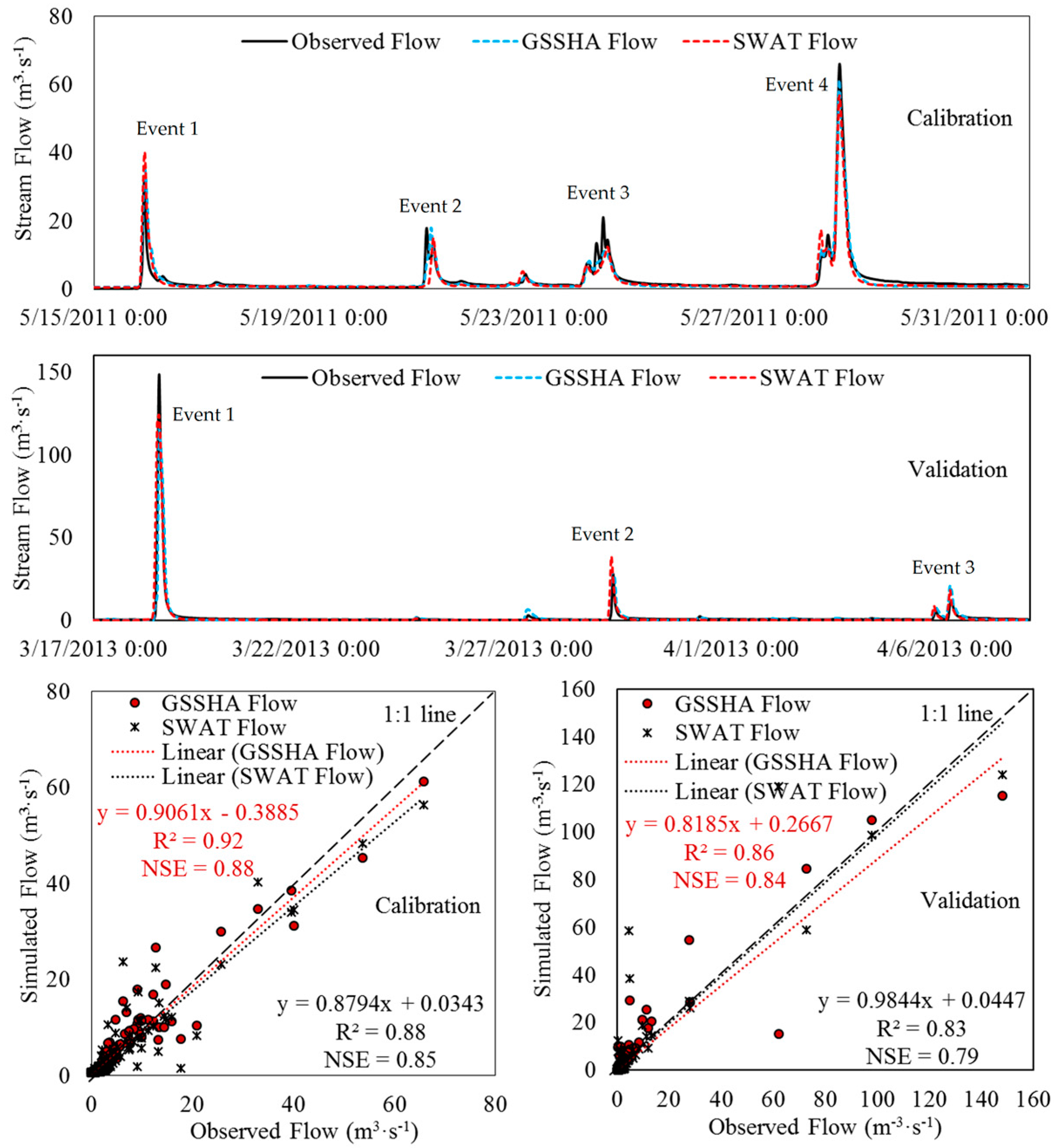
Both GSSHA and SWAT models were calibrated against observed stream flow and suspended sediment concentration on hourly temporal resolution from 15 to 31 May 2011 during which four significant flood events were observed. The models were further validated during the period of 17 March to 7 April 2013. The calibrated parameters for GSSHA stream flow simulation are shown in Table 1 and Table 2, while those for SWAT stream flow are shown in Table 3. The Web-based Hydrograph Analysis Tool (WHAT) was applied on an hourly time step for separating baseflow from surface flow using recursive digital filtering [39]. Figure 3 illustrates the comparison of baseflow values estimated by GSSHA and SWAT models along with 1:1 line during calibration and validation periods. Both models performed well in estimating baseflow in the study watershed with very good statistical agreement (R2 = 0.93, NSE = 0.90 for GSSHA and R2 = 0.90, NSE = 0.88 for SWAT) during calibration and (R2 = 0.89, NSE = 0.88 for GSSHA and R2 = 0.92, NSE = 0.88 for SWAT) during validation. Nonetheless, GSSHA gave slightly better baseflow prediction during calibration due to a fully coupled 2D groundwater flow component. The hourly simulated stream flow of GSSHA and SWAT models were also graphically compared with the observed stream flow along with 1:1 line (Figure 4). The trends of simulated stream flow in both models consistently match with the trend of observed stream flow with overall statistical performance of (R2 = 0.92, NSE = 0.88 for GSSHA and R2 = 0.88, NSE = 0.85 for SWAT) during calibration and (R2 = 0.86, NSE = 0.84 for GSSHA and R2 = 0.83, NSE = 0.79 for SWAT) during validation. The high coefficient of determination (R2) and NSE values during calibration and validation indicates satisfactory performance of both models in the study watershed. However, the GSSHA model provided slightly better predicted stream flow compared with SWAT for overall performance.
Though overall performance was satisfactory, the performances for individual flood events were also analyzed for the comparative study of both models (Table 4 and Table 5). During calibration, the errors between simulated and observed peak of four flood events estimated by GSSHA ranged from −1.30% to 4.03%, while the error estimated by SWAT varied from −16.67% to 21.86%. This indicates that GSSHA provided much better results for peak flow values compared to SWAT. In terms of volume error, both models gave similar results, yet GSSHA showed slightly better estimation of water volume due to better estimation of baseflow. In addition, the coefficient of determination (R2) and NSE for individual flood events were also analyzed to further evaluate the comparison between the two models. Reasonably high R2 > 0.60 and NSE > 0.50 could be observed for most flood events simulated by GSSHA and SWAT except for flood event 2. For flood event 2, SWAT could not accurately simulate the stream flow with relatively low R2 = 0.45 and NSE = 0.42 compared to GSSHA. This might have been caused by the different occurrence times of rising limbs between simulated and observed hydrograph. The hydrograph of flood event 2 comprised of two peaks that were generated from two instantaneous rainfall occurrences. However, the rising limb of the hydrograph generated by SWAT likely occurred at the second rainfall occurrence instead of the first one for which the SWAT model could not generate a hydrograph. In contrast, GSSHA could produce the rising limb of the hydrograph at the same time as observed. For flood event 3, although multiple peaks were also found, both models still gave much better results compared with those for flood event 2. This can be explained by the rising limb of simulated and observed hydrographs occurring at the same time, inducing small deviation at each comparison points during the flood event. From the results, along with statistical analysis between simulated and observed stream flows, it can be concluded that the fully distributed hydrologic model (GSSHA) performed slightly better than the semi-distributed model (SWAT) with new sub-daily configuration for predicting hourly stream flow in the study watershed. Golmohammadi et al. [6] also found that a fully distributed physically-based MIKE-SHE model also performed better than the semi-distributed SWAT and Agricultural Policy/Environmental Extender (APEX) model in predicting stream flow on daily basis.
During validation, all calibrated parameter values remained the same. As can be seen in Table 5, the errors between observed and simulated peaks ranged from −22.42% to 32.72 and from −16.27% to 36.86%, while the volume errors varied from −8.96% to 25.79% and from −16.30% to 10.54% for GSSHA and SWAT, respectively. Both models underestimated the extreme flood event and overestimated the small to moderate flood events. However, both models still produced good accuracies for each individual flood event with acceptable statistical criteria (R2 > 0.67, and NSE > 0.46).
3.2. Sediment Concentration
The simulated hourly sediment concentration values were graphically compared with the observed sediment concentration along with 1:1 line for both GSSHA and SWAT models during the calibration period (Figure 5). The calibrated parameters of GSSHA and SWAT for estimating sediment concentration are listed in Table 6 and Table 7, respectively. The trend of simulated values of sediment concentration followed that of the observed values for entire calibration period with R2 = 0.86, NSE = 0.83 and R2 = 0.72, NSE = 0.69 for GSSHA and SWAT, respectively. These statistical criteria indicate that GSSHA provided much better accuracy in predicting sediment concentration overall as compared with SWAT in the study watershed. Furthermore, relatively high R2 and NSE for GSSHA indicate better performance when compared with the SWAT model for individual flood events (Table 8). However, the performance of SWAT was still within the acceptable limits. The analysis of R2 and NSE for both continuous and individual flood events is likely opposite with the finding of Jeong et al.[32], which reported that SWAT with sub-daily erosion accurately predicted sediment yield in individual flood events compared to overall long-term performance in one-year simulation. However, in this study, only a half month of data was used for entire calibration. In addition to the analyses of R2 and NSE for overall and individual event performance, the deviation of sediment peak and volume were also analyzed. GSSHA was able to accurately simulate the extreme flood event (event 4) with a small peak error of −8.11%, while during the same flood event, SWAT produced a much higher peak error of −28.14%. Moreover, the higher values of peak error were found when smaller peak values occurred in both models. Conversely, small values of peak error were seen during high peak flood events. This result is consistent with the studies reported by various researchers [4,40]. Even though the SWAT model was developed to simulate sub-daily erosion by incorporating some realistic processes such as splash erosion and overland flow erosion, the model performance was still slightly low as compared with GSSHA, which also incorporates the similar erosion processes. This can be explained by how GSSHA is formulated from structured grid cells, which allow eroded sediment to be transported from cell to cell toward the stream networks and watershed outlet. Furthermore, with insufficient transport capacity, GSSHA allows sediment to be deposited within grid cells, which can be transported in succeeding flood events. On the other hand, SWAT does not incorporate the over land flow transport capacity and sediment deposition from previous flood events. Bonuma et al. [41] demonstrated that the integration of a transport capacity and sediment deposition routine in SWAT could increase the accuracy in predicting sediment yield in watersheds with steep slopes.
The period used for stream flow validation was also used for validation of the sediment concentration (Figure 5). Both models performed satisfactorily with R2 = 0.71, NSE = 0.68 and R2 = 0.82, NSE = 0.75 for GSSHA and SWAT, respectively. As can be seen in Table 9, the models significantly underestimated the SSC peak of the extreme flood event with peak errors of 33.84% and 22.50% for GSSHA and SWAT, respectively. The observed SSC during the extreme flood event was relatively low as compared to the magnitude of stream flow. This can be explained by the dominance of surface runoff on the SSC, which possibly induced the dilution effect. However, in terms of SSC peak error, both models were successfully validated for the other flood events. In addition, the volume errors were found to vary from −11.22% to 47.13% and from 32.07% to 74.66% for GSSHA and SWAT, respectively. This confirms that GSSHA provided a slightly better simulation of sediment volume for each individual flood event compared with SWAT. Even though both models had large and small errors in SSC peak and sediment volume, the statistical criteria were found to be within the acceptable limits (R2 > 0.60 and NSE > 0.48).
3.3. Evaluation of Model Performance for Long-Term Simulation
The long-term simulation was carried out during the period 2011–2013 and the parameter values for stream flow and SSC from the calibration and validation remained the same during the simulation. Figure 6 shows the comparison of hourly observed and simulated stream flow in the study watershed during the period 2011–2013. Both models successfully predicted the hourly stream flow with a good statistical agreement R2 = 0.71 and NSE = 0.63 for GSSHA and R2 = 0.67 and NSE = 0.49 for SWAT, respectively. However, over the entire simulation, the models either underestimated or overestimated the peak stream flow. In the study watershed, the hydrological response is always characterized by numerous episodic rainfall events [42], resulting in difficulties for long-term simulation. Based on the R2 values, both models yielded comparable results. However, the NSE of SWAT was better than that of GSSHA. This shows that, although the prediction from both models followed the trends of the observed stream flow data, the relative magnitude of residual variance in GSSHA was relatively higher as compared with that in SWAT. Moreover, an interesting observation was that GSSHA frequently produced a large number of very small flood events, which also possibly caused the high relative magnitude of residual variance.
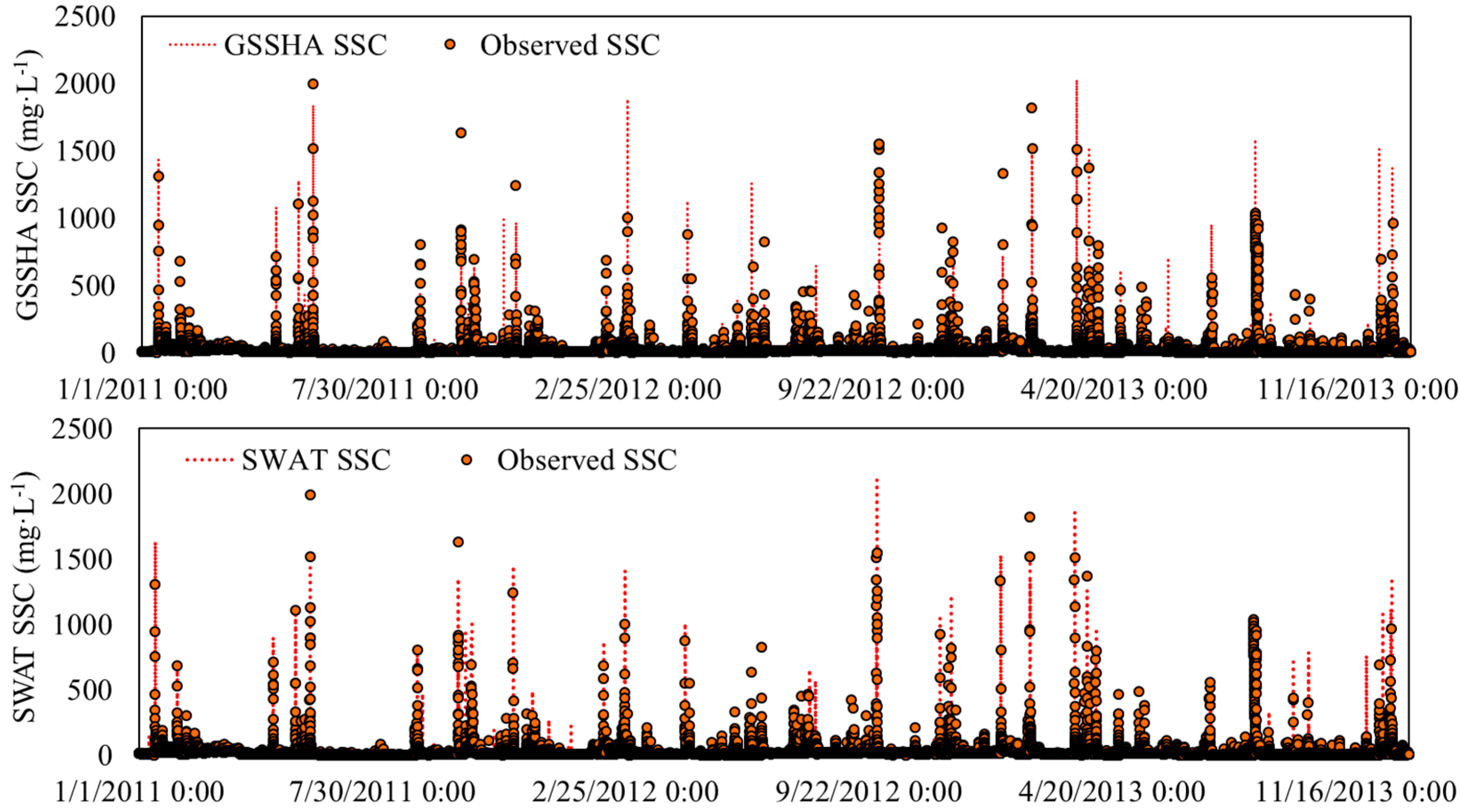
Observed and simulated hourly SSC using GSSHA and SWAT models are presented in Figure 7. In general, the simulation of sediment concentration was found to be more difficult compared with that of sediment load. However, both models successfully predicted the SSC during a long-term period (2011–2013) with acceptable statistical criteria of R2 = 0.44, NSE = 0.41 and R2 = 0.58, NSE = 0.47 for GSSHA and SWAT, respectively. Based on the statistical criteria, SWAT performed better in predicting SSC. This can be partly explained by the fact that GSSHA was designed for event-based simulation and does not incorporate crop cultivation management schemes (planting, harvesting schedule, tillage activities, etc.), which is a significant factor controlling sediment transport in the intensively agricultural watershed. Although a new sub-daily algorithm is likely able to realistically predict sub-daily erosion in a small watershed [32], SWAT is still not able to consider the overland deposited sediment generated from previous flood events and allows all soil eroded by overland flow to reach the stream networks and watershed outlet directly. However, in the study watershed, Sith et al. [42] indicated that, during flood events, the suspended sediment was significantly transported from deposited sources generated from previous flood events. This shows the lack of incapability in SWAT for simulating the sediment transport as compared to GSSHA.
4. Conclusions
This study evaluates the performances of two hydrologic models, namely, GSSHA and SWAT, in predicting hourly stream flow and suspended sediment concentration in a small predominantly agricultural watershed. The two models require almost the same data input and model parameters. Both models were calibrated against hourly stream flow and sediment concentration for the period of 15 to 31 May 2011 and validated for a period of 17 March to 7 April 2013. From the results of this study, the GSSHA model performed slightly better than the SWAT model in simulating hourly stream flow. Furthermore, GSSHA provided more accurate results of hourly sediment concentration, particularly during extreme flood events. However, the performance of SWAT with sub-daily erosion in predicting sediment concentration was still satisfactory. In addition, this study reveals that GSSHA, as a fully distributed model with structured grid cells, provided better results in predicting sediment concentration compared with SWAT, as a semi-distributed model, even though SWAT has been recently developed by incorporating more realistic sediment transport processes such as splash and overland erosion. Differences in the calibration method for each model may also be partly causing the differences in the model output. Aside from short-term simulations, the performances of both models were also evaluated through long-term simulations by comparing the observed and simulated hourly stream flow and sediment concentration. Both models yielded the comparable results for both stream flow and SSC with acceptable agreement in the study watershed. However, SWAT performed better in predicting long-term SSC as compared with GSSHA. This indicates the lack of incapability in GSSHA for simulating crop cultivation management practices, which are the key determinants of sediment transport in an intensively agricultural watershed. Overall, both models were able to simulate hydrological and sediment transport processes in the small watershed scale in a satisfactory way, although the performance of the SWAT model was found to be slightly less accurate than that of GSSHA for short-term simulations. However, for the long-term simulation, SWAT performed slightly better in predicting sediment concentration.
Acknowledgments
This research was financially supported by the Environment Research and Technology Development Fund (4-1304) of the Ministry of the Environment, Japan Society for the Promotion of Science (JSPS) Grant-in-Aids for Scientific Research (No. 15H02268, and 25257305), the JSPS Japan–Philippines Research Cooperative Program, and the doctoral research scholarship from Southeast Asia Engineering Education Development Network Project (AUN/SEED-Net JICA) program.
Author Contributions
Ratino Sith was responsible in analyzing the data and writing the manuscript; Kazuo Nadaoka helped in reviewing and editing the manuscript.
Conflicts of Interest
The authors declare no conflict of interest.
References
- Bobba, A.G.; Singh, V.P.; Bengtsson, L. Application of environmental models to different hydrological systems. Ecol. Model. 2000, 125, 15–49. [Google Scholar] [CrossRef]
- Borah, D.K.; Bera, M. Watershed-scale hydrologic and nonpoint-source pollution models: Review of mathematical bases. Trans. ASAE 2003, 46, 1553–1566. [Google Scholar] [CrossRef]
- Borah, D.K.; Arnold, J.G.; Bera, M.; Krug, E.C.; Liang, X.Z. Storm event and continuous hydrologic modeling for comprehensive and efficient watershed simulations. J. Hydrol. Eng. 2007, 12, 605–616. [Google Scholar] [CrossRef]
- Shen, Z.Y.; Gong, Y.W.; Li, Y.H.; Hong, Q.; Xu, L.; Liu, R.M. A comparison of WEPP and SWAT for modeling soil erosion of the Zhangjiachong watershed in the Three Gorges reservoir area. Agric. Water Manag. 2009, 96, 1435–1442. [Google Scholar] [CrossRef]
- Paudel, M.; Nelson, E.J.; Downer, C.W.; Hotchkiss, R. Comparing the capability of distributed and lumped hydrologic models for analyzing the effects of land use change. J. Hydroinform. 2011, 13, 461–473. [Google Scholar] [CrossRef]
- Golmohammadi, G.; Prasher, S.; Madani, A.; Rudra, R. Evaluating three hydrological distributed watershed models: MIKE–SHE, APEX, SWAT. Hydrology 2014, 1, 20–39. [Google Scholar] [CrossRef]
- Downer, C.W.; Ogden, F.L.; Martin, W.D.; Harmon, R.S. Theory, development and applicability of the surface water hydrologic model CASC2D. Hydrol. Process. 2002, 16, 255–275. [Google Scholar] [CrossRef]
- Arnold, J.G.; Williams, J.R.; Srinivasan, R.; King, K.W.; Griggs, R.H. SWAT: Soil and Water Assessment Tool; USDA Agricultural Research Service: College Station, TX, USA, 1994. [Google Scholar]
- HEC 2001 HEC-HMS, User’s Mannual, Version 2.1; US Army Corps of Engineerings Hydrologic Engineering Center: Davis, CA, USA, 2001.
- Sharif, H.O.; Sparks, L.; Hassan, A.A.; Zeitler, J.; Xie, H. Application of a distributed hydrologic model to the November 17, 2004, fllod of Bull Creek watershed, Austin, Texas. J. Hydrol. Eng. 2010, 15, 651–657. [Google Scholar] [CrossRef]
- Sharif, H.O.; Hassan, A.A.; Shafique, S.B.; Xie, H.; Zeitler, J. Hydrologic modeling of an extreme flood in the Guadalupe river in Texas. J. Am. Water Resour. Assoc. 2010, 46, 881–891. [Google Scholar] [CrossRef]
- Pradhan, N.R.; Downer, C.W.; Johnson, B.E. A physics based hydrologic modeling approach to simulate non–point source pollution for the purposes of calculating TMDLs and designing abatement measures. In Practical Aspects of Computational Chemistry III; Leszczynski, J., Shukla, M.K., Eds.; Springer US: New York, NY, USA, 2014; pp. 249–282. [Google Scholar]
- Arnold, J.G.; Allen, P.M. Methods for estimating baseflow and groundwater recharge from stream flow. J. Am. Water Resour. Assoc. 1999, 35, 411–424. [Google Scholar] [CrossRef]
- Gassman, P.W.; Reyes, M.R.; Green, C.H.; Arnold, J.G. The soil and water assessment tool: Historical development, application, and future research directions. Trans. ASABE 2007, 50, 1211–1250. [Google Scholar] [CrossRef]
- Neitsch, S.L.; Arnold, J.G.; Kiniry, J.R.; Williams, J.R. Soil and Water Assessment Tool: Theoretical Documentation—Version 2009; Grassland, Soil and Water Research Laboratory, Agricultural Research Service: College Station, TX, USA, 2009; p. 618. [Google Scholar]
- Im, S.; Brannan, K.; Mostaghimi, S.; Cho, J. A comparison of SWAT and HSPF models for simulating hydrologic and water quality responses from an urbanizing watershed. In Proceedings of the 2003 ASAE Annual Meeting, Las Vegas, NV, USA, 27–30 July 2003. [Google Scholar]
- Abu El-Nasr, A.; Arnold, J.G.; Feyen, J.; Berlamont, J. Modeling the hydrology of a catchment using a distributed and a semi distributed model. Hydrol. Process. 2005, 19, 573–587. [Google Scholar] [CrossRef]
- Diluzio, M.; Arnold, J.G. Formulation of a hybrid calibration approach for a physically based distributed model with NEXRAD data input. J. Hydrol. 2004, 298, 136–154. [Google Scholar] [CrossRef]
- Jeong, J.; Kannan, N.; Arnold, J.; Glick, R.; Gosselink, L.; Srinivasa, R. Development and integration of sub-hourly rainfall-runoff modeling capability within a watershed model. Water Resour. Manag. 2010, 24, 4505–4527. [Google Scholar] [CrossRef]
- Maharjan, G.R.; Park, Y.S.; Kim, N.W.; Shin, D.S.; Choi, J.W.; Hyun, G.W.; Jeon, J.H.; Ok, Y.S.; Lim, K.J. Evaluation of SWAT sub-daily runoff estimation at small agricultural watershed in Korea. Front. Environ. Sci. Eng. 2013, 7, 109–119. [Google Scholar] [CrossRef]
- Yang, X.; Liu, Q.; He, Y.; Luo, X.; Zhang, X. Comparison of daily and sub-daily SWAT models for daily stream flow simulation in the Upper Huai River Basin of China. Stoch. Environ. Res. Risk Assess. 2016, 30, 959–972. [Google Scholar] [CrossRef]
- Chintalapudi, S.; Sharif, H.O.; Xie, H. Sensitivity of distributed hydrlogic simulations to ground and satellite based rainfall products. Water 2014, 6, 1221–1245. [Google Scholar] [CrossRef]
- Saha, G.C. Climate change induced precipitation effects on water resources in the Peace region of British Columbia, Canada. Climate 2015, 3, 264–282. [Google Scholar] [CrossRef]
- Downer, C.W.; Ogden, F.L. GSSHA: Model to simulate diverse stream flow producing processes. J. Hydrol. Eng. 2004, 9, 161–174. [Google Scholar] [CrossRef]
- Downer, C.W.; Pradhan, N.R.; Ogden, F.L.; Byrd, A.R. Testing the effects of detachment limits and transport capacity formulation on sediment runoff predictions using the U.S. Army Corps of Engineering GSSHA model. J. Hydrol. Eng. 2015, 20, 1–11. [Google Scholar] [CrossRef]
- Chow, V.T.; Maidment, D.R.; Mays, L.W. Applied Hydrology; McGrawHill: New York, NY, USA, 1998. [Google Scholar]
- Cunge, J.A. On the subject of a flood propagation method (Muskingum method). J. Hydraul. Res. 1969, 7, 205–230. [Google Scholar] [CrossRef]
- Williams, J.R. Flood routing with variable travel time or variable storage coefficients. Trans. ASABE 1969, 12, 100–103. [Google Scholar] [CrossRef]
- Arnold, J.G.; Allen, P.M.; Bernhardt, G. A comprehensive surface-groundwater flow model. J. Hydrol. 1993, 142, 47–69. [Google Scholar] [CrossRef]
- Monteith, J.L. Evaporation and the environment: In the state and movement of water in living organisms. Symp. Soc. Exp. Biol. 1965, 19, 205–234. [Google Scholar] [PubMed]
- Williams, J.R. Sediment-yield prediction with universal equation using runoff energy factor. In Present and Prospective Technology for Predicting Sediment Yield and Sources, Proceedings of the Sediment Yield Workshop, 28–30 November 1972; Agriculture Research Service, US Department of Agriculture: College Station, TX, USA, 1975; pp. 244–252. [Google Scholar]
- Jeong, J.; Kannan, N.; Arnold, J.G.; Glick, R.; Gosselink, L.; Srinivasan, R.; Harmel, R.D. Development of sub-daily erosion and sediment transport algorithms for SWAT. Trans. ASABE 2010, 54, 1685–1691. [Google Scholar] [CrossRef]
- Abbaspour, K.C. SWAT-CUP: SWAT Calibration and Uncertainty Programs—A User Manual; Swiss Federal Institute of Aquatic Science and Technology, Eawag: Dübendorf, Switzerland, 2011. [Google Scholar]
- Tolson, B.A.; Shoemaker, C.A. Dynamically dimensioned search algorithm for computationally efficient watershed model calibration. Water Resour. Res. 2007, 43, 1–16. [Google Scholar] [CrossRef]
- Santhi, C.; Arnold, J.G.; Williams, J.R.; Dugas, W.A.; Srinivasan, R.; Hauck, L.M. Validation of the SWAT model on a large river basin with point and nonpoint sources. J. Am. Water Res. Assoc. 2001, 37, 1169–1188. [Google Scholar] [CrossRef]
- Van Liew, M.W.; Garbrecht, J. Hydrological simulation of the little Washita river experimental watershed using SWAT. J. Am. Water Res. Assoc. 2003, 39, 413–426. [Google Scholar] [CrossRef]
- Nash, J.E.; Sutchliffe, J.V. River flow forecasting through conceptual models. Part 1-A discussion of principles. J. Hydrol. 1970, 10, 282–290. [Google Scholar] [CrossRef]
- Krause, P.; Boyle, D.P.; Base, F. Comparision of different efficiency criteria for hydrological model assessment. Adv. Geosci. 2005, 5, 83–87. [Google Scholar] [CrossRef]
- Lim, K.J.; Engel, B.A. WHAT: Web-based Hydrograph Analysis Tool. Available online: https://engineering.purdue.edu/mapserve/WHAT/ (accessed on 10 December 2016).
- Nearing, M.A.; Govers, G.; Norton, L.D. Variability in soil erosion data from replicated plots. Soil Sci. Soc. Am. J. 1999, 63, 1829–1835. [Google Scholar] [CrossRef]
- Bonuma, N.B.; Rossi, C.G.; Arnold, J.G.; Reichert, J.M.; Minella, J.P.; Allen, P.A.; Volk, M. Simulating landscape sediment transport capacity by using modified SWAT model. J. Environ. Qual. 2014, 43, 55–66. [Google Scholar] [CrossRef] [PubMed]
- Sith, R.; Yamamoto, T.; Watanabe, A.; Nakamura, T.; Nadaoka, K. Analysis of red soil sediment yield in a small agricultural watershed in Ishigaki Island, Japan, using long-term and high resolution monitoring data. Environ. Process. 2017, 4, 1–22. [Google Scholar] [CrossRef]
Figure 1.
Todoroki watershed study site, Ishigaki Island, Okinawa, Japan.
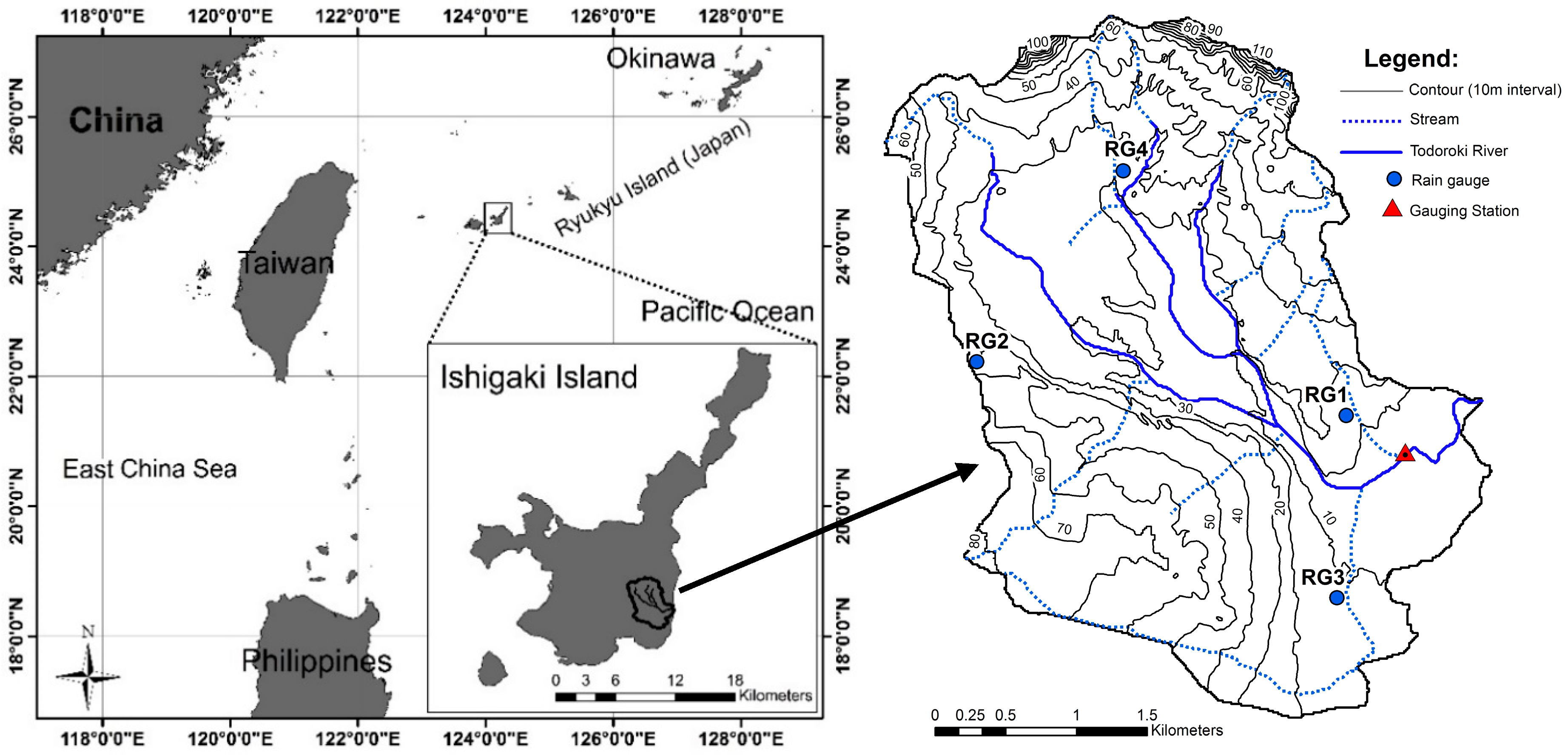
Figure 2.
(a) Todoroki watershed land cover; (b) soil type; (c) subsurface geological information.

Figure 3.
Comparison between calculated and simulated baseflow for Todoroki watershed.
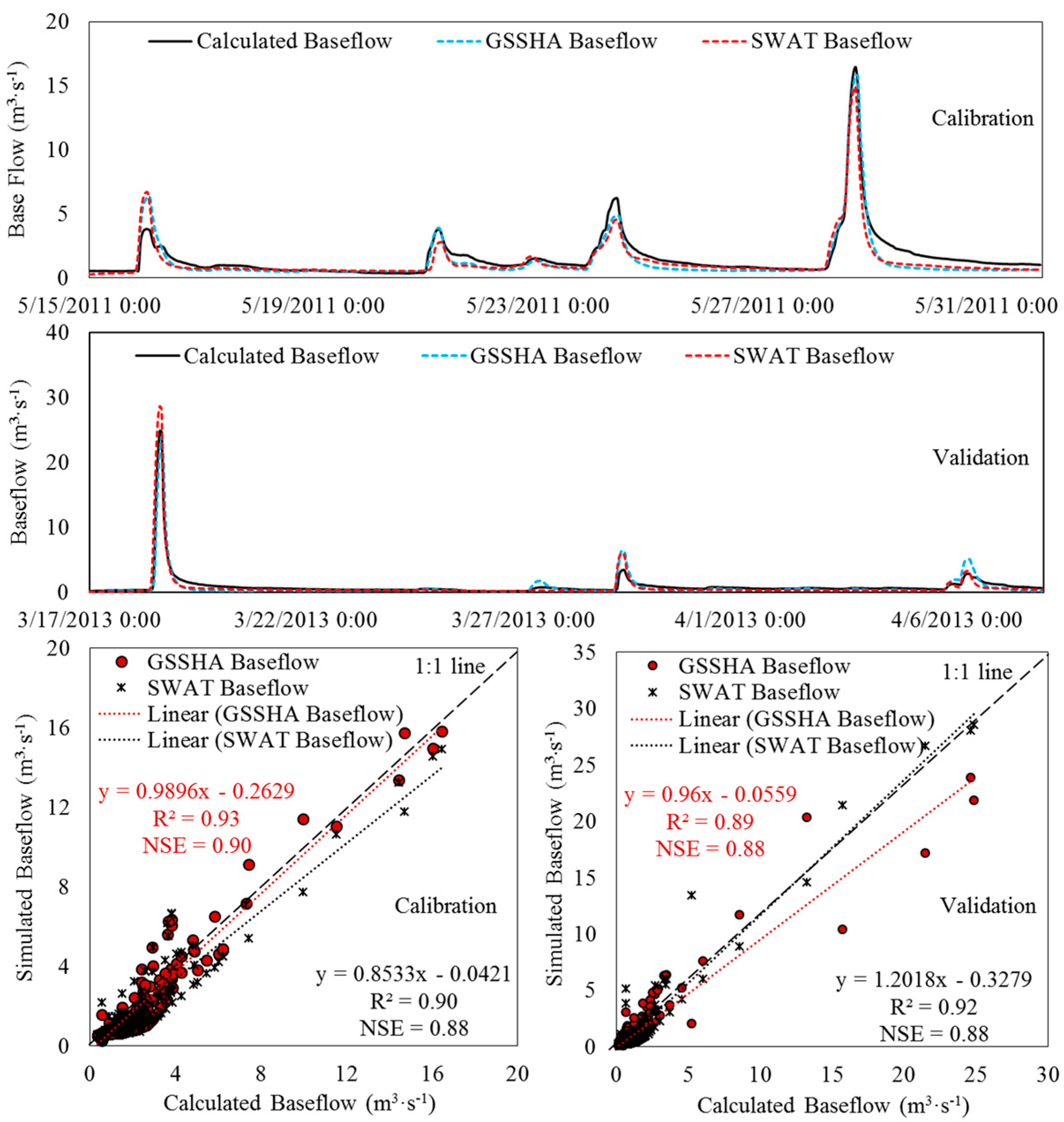
Figure 4.
Comparison between observed and simulated stream flow for Todoroki watershed.

Figure 5.
Comparison between observed and simulated suspended sediment concentration in Todoroki watershed.
Figure 5.
Comparison between observed and simulated suspended sediment concentration in Todoroki watershed.
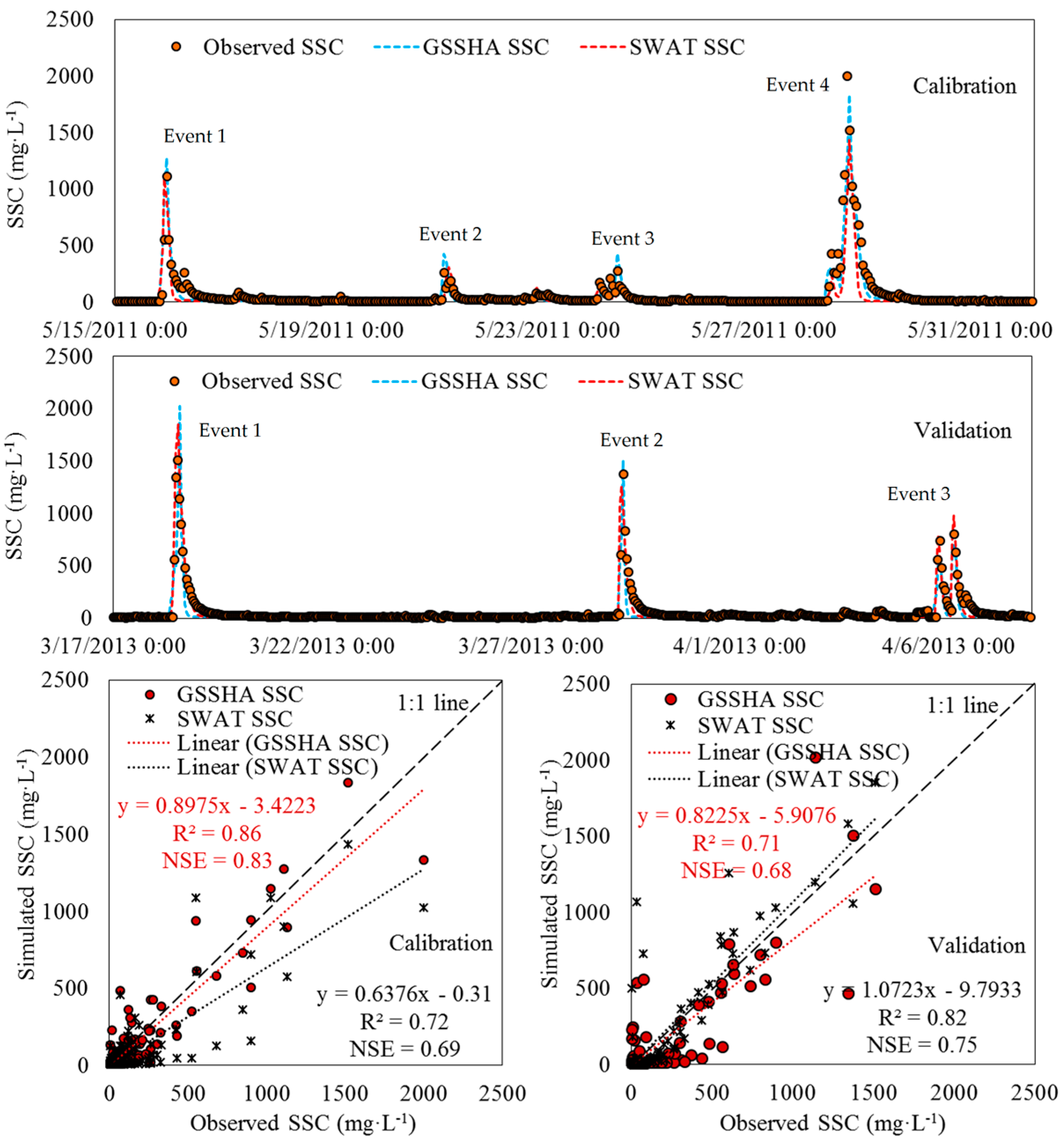
Figure 6.
Comparison between observed and simulated long-term stream flow predicted by GSSHA and SWAT models during (2011–2013) in Todoroki watershed.
Figure 6.
Comparison between observed and simulated long-term stream flow predicted by GSSHA and SWAT models during (2011–2013) in Todoroki watershed.
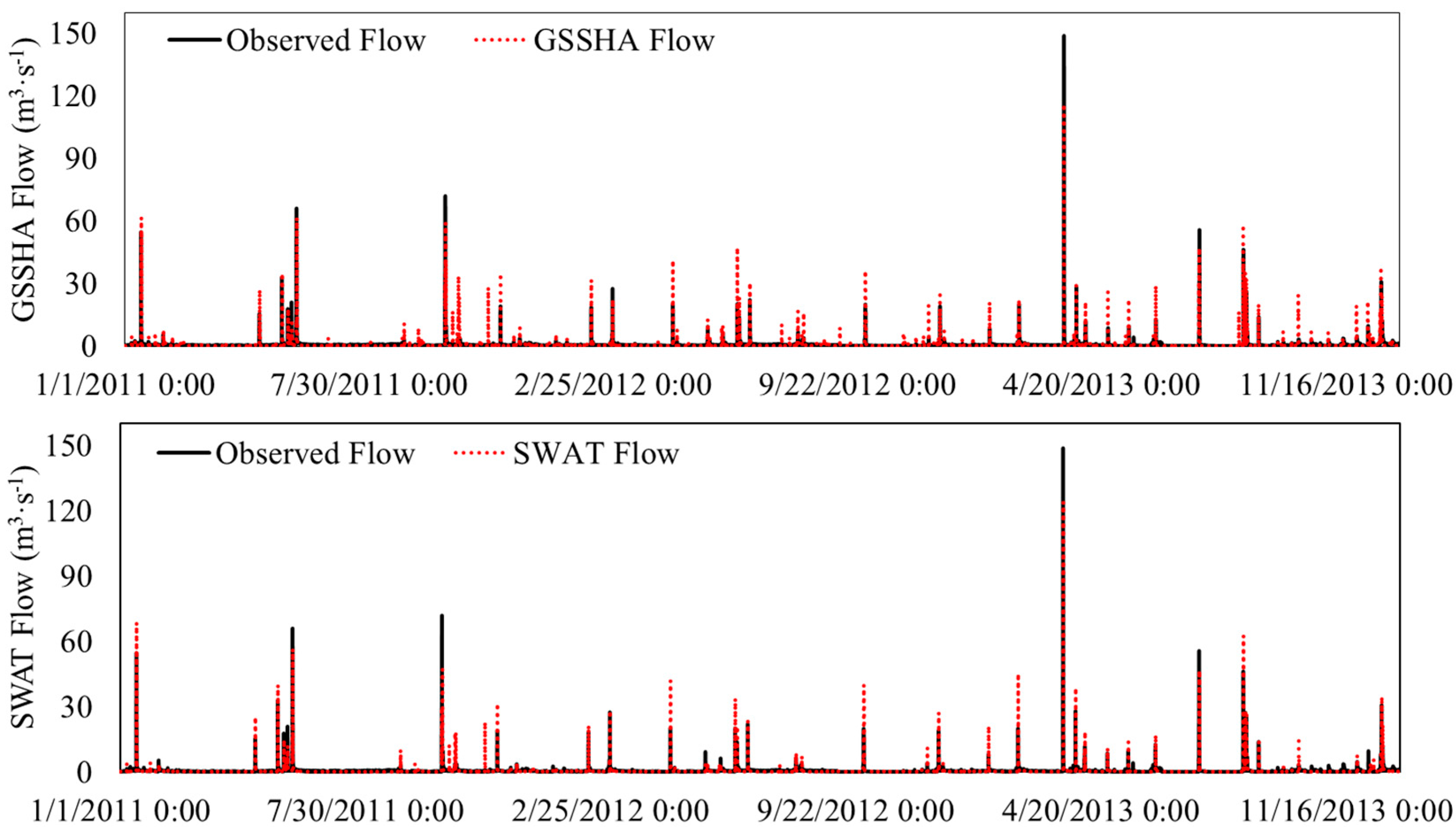
Figure 7.
Comparison between observed and simulated long-term SSC predicted by GSSHA and SWAT models during (2011–2013) in Todoroki watershed.
Figure 7.
Comparison between observed and simulated long-term SSC predicted by GSSHA and SWAT models during (2011–2013) in Todoroki watershed.

Table 1.
Soil hydrologic properties used in the GSSHA model calibration of stream flow.
| Parameters | Alluvial | Kunigami | Shimajiri |
|---|---|---|---|
| Hydraulic conductivity (cm·h−1) | 0.12 | 0.40 | 0.36 |
| Capillary head (cm) | 28.25 | 35.3 | 32.20 |
| Porosity (m3·m−3) | 0.35 | 0.295 | 0.295 |
| Pore distribution index (cm·cm−1) | 0.256 | 0.378 | 0.378 |
| Residual saturation (m3·m−3) | 0.056 | 0.056 | 0.056 |
| Field capacity (m3·m−3) | 0.131 | 0.127 | 0.128 |
| Wilting point (m3·m−3) | 0.10 | 0.10 | 0.10 |
| Initial moisture (m3·m−3) | 0.22 | 0.20 | 0.20 |
Table 2.
Manning’s surface roughness values used in the GSSHA model calibration of stream flow.
| Parameters | Manning’s Roughness |
|---|---|
| Open water | 0.090 |
| Built-up | 0.015 |
| Bare land | 0.105 |
| Forest | 0.204 |
| Grassland | 0.175 |
| Pasture | 0.180 |
| Paddy field | 0.150 |
| Pineapple | 0.120 |
| Sugarcane | 0.210 |
| Other agricultural farmland | 0.160 |
Table 3.
Parameters used in the SWAT model calibration of stream flow.
| Parameters | Definition | Range | Fitted Values |
|---|---|---|---|
| v_SURLAG.bsn | Surface runoff lag coefficient | 1–24 | 10.32 |
| v_EPCO.bsn | Plant uptake compensation factor | 0.01–1 | 0.607 |
| v_ALPHA_BF.gw | Base flow alpha factor | 0–1 | 0.385 |
| v_RCHRG_DP.gw | Deep aquifer percolation fraction | 0–1 | 0.767 |
| v_GW_DELAY.gw | Groundwater delay | 0–350 | 162 |
| v_GWQMN.gw | Threshold depth of water in the shallow aquifer for return flow to occur | 10–1000 | 576 |
| v_REVAPMN.gw | Threshold depth of water in the shallow aquifer for “revap” to occur | 0–100 | 98 |
| v_GW_REVAP.gw | Groundwater “revap” coefficient | 0.02–0.2 | 0.125 |
| v_OV_N.hru | Manning’s “n” value for overland flow | 0.01–0.8 | 0.738 |
| r_SOL_AWC.sol | Available water capacity of the soil layer | −0.3–0.3 | 0.118 |
| r_SOL_K.sol | Saturated hydraulic conductivity (mm/h) | −0.8–0.8 | −0.689 |
| r_SOL_BD.sol | Moisture bulk density | −0.3–0.3 | −0.185 |
| v_ESCO.bsn | Soil evaporation compensation factor | 0.01–1 | 0.237 |
| v_CH_N2.rte | Manning’s “n” value for the main channel | 0.01–0.5 | 0.319 |
| v_CH_K2.rte | Effective hydraulic conductivity in main channel | 0–150 | 129 |
v_: means the default parameter is replaced by a given value, and r_ means the existing parameter value is multiplied by (1 + a given value).
Table 4.
Statistical analysis of observed and simulated stream flow for single flood events during calibration.
Table 4.
Statistical analysis of observed and simulated stream flow for single flood events during calibration.
| Models | Events | Observed Peak (m3·s−1) | Simulated Peak (m3·s−1) | Peak Error (%) | Observed Volume (m3) | Simulated Volume (m3) | Volume Error (%) | R2 | NSE |
|---|---|---|---|---|---|---|---|---|---|
| GSSHA | Event 1 | 32.99 | 34.32 | 4.03 | 585,225 | 733,707 | 25.37 | 0.87 | 0.69 |
| Event 2 | 17.76 | 17.53 | −1.30 | 606,637 | 549,346 | −9.44 | 0.68 | 0.65 | |
| Event 3 | 7.46 | 7.76 | 4.02 | 831,538 | 637,851 | −23.29 | 0.88 | 0.81 | |
| Event 4 | 65.74 | 60.87 | −7.41 | 1,755,397 | 1,538,002 | −12.38 | 0.97 | 0.96 | |
| SWAT | Event 1 | 32.99 | 40.2 | 21.86 | 585,225 | 758,887 | 29.67 | 0.87 | 0.58 |
| Event 2 | 17.76 | 14.8 | −16.67 | 606,637 | 492,080 | −18.88 | 0.45 | 0.42 | |
| Event 3 | 7.46 | 6.84 | −8.31 | 831,538 | 659,369 | −20.70 | 0.83 | 0.75 | |
| Event 4 | 65.74 | 56.1 | −14.66 | 1,755,397 | 1,462,968 | −16.66 | 0.95 | 0.92 |
Table 5.
Statistical analysis of observed and simulated stream flow for single flood events during validation.
Table 5.
Statistical analysis of observed and simulated stream flow for single flood events during validation.
| Models | Events | Observed Peak (m3·s−1) | Simulated Peak (m3·s−1) | Peak Error (%) | Observed Volume (m3) | Simulated Volume (m3) | Volume Error (%) | R2 | NSE |
|---|---|---|---|---|---|---|---|---|---|
| GSSHA | Event 1 | 148.24 | 115.01 | −22.42 | 1,885,258 | 1,716,390 | −8.96 | 0.89 | 0.88 |
| Event 2 | 28.13 | 29.17 | 3.70 | 555,687 | 698,999 | 25.79 | 0.74 | 0.71 | |
| Event 3 | 15.86 | 21.05 | 32.72 | 559,162 | 657,299 | 17.55 | 0.86 | 0.68 | |
| SWAT | Event 1 | 148.24 | 124.12 | −16.27 | 1,885,258 | 2,083,882 | 10.54 | 0.84 | 0.82 |
| Event 2 | 28.13 | 38.5 | 36.86 | 555,687 | 599,490 | 7.88 | 0.82 | 0.46 | |
| Event 3 | 15.86 | 18.6 | 17.28 | 559,162 | 468,029 | −16.30 | 0.67 | 0.58 |
Table 6.
Parameters used in the GSSHA model calibration of sediment concentration.
| Land Cover | Soil Type | Erodibility Coefficient (K) | Detachment Coefficient (1·J−1) | Rill Erodibility Coefficient (s·m−1) |
|---|---|---|---|---|
| Sugarcane | Alluvial | 0.00362 | 7.95 | 0.1529 |
| Sugarcane | Kunigami | 0.00826 | 14.16 | 0.0924 |
| Sugarcane | Shimajiri | 0.00684 | 15.32 | 0.0638 |
| Pasture | Alluvial | 0.00236 | 8.27 | 0.0527 |
| Pasture | Kunigami | 0.000328 | 10.16 | 0.0426 |
| Pasture | Shimajiri | 0.000267 | 9.56 | 0.0582 |
| Pineapple | Kunigami | 0.03572 | 21.86 | 0.2548 |
| Others | Alluvial | 0.000154 | 5.27 | 0.0527 |
| Others | Kunigami | 0.000217 | 9.57 | 0.0532 |
| Others | Shimajiri | 0.000359 | 10.38 | 0.0624 |
Table 7.
Parameters used in the SWAT model calibration of sediment concentration.
| Parameters | Definition | Range | Fitted Values |
|---|---|---|---|
| v_CH_COV1.rte | Channel erodibility factor | 0–0.6 | 0.5 |
| v_CH_COV2.rte | Channel cover factor | 0.001–1 | 1 |
| v_SPCON.bsn | Linear factor for channel sediment routing | 0.0001–0.01 | 0.005 |
| v_SPEXP.bsn | Sediment re-entrained in channel sediment routing | 1–1.5 | 1.2 |
| v_EROS_EXPO.bsn | Exponent in the overland flow erosion equation | 1–3 | 1.2 |
| v_EROS_SPL.bsn | Splash erosion coefficient | 0.9–3.1 | 1.5 |
| v_C_FACTOR.bsn | Parameter for cover and management factor P | 0.001–0.45 | 0.40 |
| v_PRF_BSN.bsn | Peak rate adjustment factor for main channel | 0–2 | 0.25 |
| v_RILLMLT.bsn | Multiplier to USLE_K for soil susceptible to rill erosion | 0.5–2 | 1.10 |
| v_CH_D50.bsn | Median particle diameter of channel bed | 0.001–10 | 5.2 |
v_: means the default parameter is replaced by a given value, and r_ means the existing parameter value is multiplied by (1 + a given value).
Table 8.
Statistical analysis of observed and simulated SSC for single flood events during calibration.
Table 8.
Statistical analysis of observed and simulated SSC for single flood events during calibration.
| Models | Events | Observed Peak (mg·L−1) | Simulated Peak (mg·L−1) | Peak Error (%) | Observed Load (ton) | Simulated Load (ton) | Load Error (%) | R2 | NSE |
|---|---|---|---|---|---|---|---|---|---|
| GSSHA | Event 1 | 1108.99 | 1272.39 | 14.73 | 159.79 | 209.65 | 31.20 | 0.85 | 0.73 |
| Event 2 | 262.25 | 425.12 | 62.10 | 40.18 | 55.30 | 37.63 | 0.58 | 0.38 | |
| Event 3 | 276.43 | 428.11 | 54.87 | 65.09 | 62.73 | −3.63 | 0.79 | 0.62 | |
| Event 4 | 1996.8 | 1834.93 | −8.11 | 1382.94 | 1142.01 | −17.42 | 0.90 | 0.89 | |
| SWAT | Event 1 | 1108.99 | 1090.24 | −1.69 | 159.79 | 189.83 | 18.80 | 0.69 | 0.60 |
| Event 2 | 262.25 | 311.23 | 18.68 | 40.18 | 46.42 | 15.53 | 0.49 | 0.28 | |
| Event 3 | 276.43 | 154.87 | −43.97 | 65.09 | 32.97 | −49.35 | 0.49 | 0.47 | |
| Event 4 | 1996.8 | 1434.93 | −28.14 | 1382.94 | 880.15 | 31.20 | 0.79 | 0.70 |
Table 9.
Statistical analysis of observed and simulated SSC for single flood events during validation.
Table 9.
Statistical analysis of observed and simulated SSC for single flood events during validation.
| Models | Events | Observed Peak (mg·L−1) | Simulated Peak (mg·L−1) | Peak Error (%) | Observed Load (ton) | Simulated Load (ton) | Load Error (%) | R2 | NSE |
|---|---|---|---|---|---|---|---|---|---|
| GSSHA | Event 1 | 1510.27 | 2021.32 | 33.84 | 1874.29 | 1663.93 | −11.22 | 0.70 | 0.66 |
| Event 2 | 1372.86 | 1505.26 | 9.64 | 220.30 | 316.54 | 43.69 | 0.73 | 0.59 | |
| Event 3 | 797.6 | 720.27 | −9.70 | 124.81 | 183.64 | 47.13 | 0.71 | 0.54 | |
| SWAT | Event 1 | 1510.27 | 1850.12 | 22.50 | 1874.29 | 2475.35 | 32.07 | 0.98 | 0.94 |
| Event 2 | 1372.86 | 1260.25 | −8.20 | 220.30 | 384.77 | 74.66 | 0.60 | 0.48 | |
| Event 3 | 797.7 | 974.38 | 22.15 | 124.81 | 182.28 | 46.04 | 0.70 | 0.55 |
© 2017 by the authors. Licensee MDPI, Basel, Switzerland. This article is an open access article distributed under the terms and conditions of the Creative Commons Attribution (CC BY) license (http://creativecommons.org/licenses/by/4.0/).
Share and Cite
MDPI and ACS Style
Sith, R.; Nadaoka, K. Comparison of SWAT and GSSHA for High Time Resolution Prediction of Stream Flow and Sediment Concentration in a Small Agricultural Watershed. Hydrology 2017, 4, 27. https://doi.org/10.3390/hydrology4020027
AMA Style
Sith R, Nadaoka K. Comparison of SWAT and GSSHA for High Time Resolution Prediction of Stream Flow and Sediment Concentration in a Small Agricultural Watershed. Hydrology. 2017; 4(2):27. https://doi.org/10.3390/hydrology4020027
Chicago/Turabian StyleSith, Ratino, and Kazuo Nadaoka. 2017. "Comparison of SWAT and GSSHA for High Time Resolution Prediction of Stream Flow and Sediment Concentration in a Small Agricultural Watershed" Hydrology 4, no. 2: 27. https://doi.org/10.3390/hydrology4020027
Note that from the first issue of 2016, this journal uses article numbers instead of page numbers. See further details here.