Corporate Cash Holdings and Exposure to Macroeconomic Conditions

Abstract

Determinants of a firm’s cash holdings have been a popular topic of research in finance, especially after the rapid surge in cash holdings for U.S. firms since the 1980s. The wide array of research has focused primarily on firm-specific factors to explain the cross-sectional variations but has found insufficient explanatory power for the variations in cash holdings. We incorporate variables for macroeconomic conditions and uncertainty with firm-specific variables. Using 19,223 firms with 213,663 firm-year observations from 1971 to 2019 and introducing five variables for macroeconomic conditions of the Aruoba–Diebold–Scotti index and three variables for macroeconomic and financial uncertainty, we find that a firm’s sensitivity to macroeconomic conditions and uncertainty plays important role in determining the level of cash holdings. We find supportive evidence from the robustness test with the firm’s age that variables for macroeconomic variables have an impact on the level of cash holdings irrespective of the firm’s age.

1. Introduction

Over recent decades, firms have accumulated unusually high levels of cash, which has amassed much attention in both academia and practitioners. Foley et al. (2007), Bates et al. (2009), Sánchez and Yurdagul (2013), Graham and Leary (2018), and Chung et al. (2020) documented this growing tendency to hold more cash holdings. For example, Bates et al. (2009) found that the average cash ratio has drastically increased from 10.5% in 1980 to 23.2% in 2006. Sánchez and Yurdagul (2013) confirmed the growing tendency in aggregate cash holdings from 1995 to 2010. Figure 1 illustrates the average cash ratio over time in the U.S. economy since 1971 and confirms that firms have been gradually accumulating their cash levels. Chung et al. (2020) stated that, especially after the 2008 financial crisis, corporate top management tends to hoard excessive cash to entrench themselves at the expense of investors and shareholders. From a more holistic point of view, there has been substantial variation in aggregate cash holdings over the century. After the highest level in the 1920s, the aggregate cash holdings fell drastically, sometimes gradually, and increased (Graham and Leary 2018). Therefore, the subsequential research agenda is to explore factors that explain these variations in the level of corporate cash holdings. Researchers have considered theoretical frameworks and identified determinants such as firm-specific characteristics to address the increasing growth in corporate cash holdings.

However, there has not been enough consensus on whether firm-specific variables have sufficient power to explain the time-series pattern in the level of cash holdings. (Opler et al. 1999; Harford et al. 2008; Denis and Sibilkov 2010; Subramaniam et al. 2011; Brisker et al. 2013; Qiu and Wan 2015; Chen et al. 2015; Tahir et al. 2016; Bates et al. 2018; Liu et al. 2021). Graham and Leary (2018) explored whether cross-sectional firm-specific variables can explain time-series changes in cash holdings and found that firm-specific variables do not explain much of the time-series changes in cash holdings. Although the theoretical framework has been empirically constructed well, what can influence cash holdings if firm characteristics do not attribute to the changes in cash holdings? What can determine the time-series changes in cash holdings? One potential candidate is variables for macroeconomic conditions. The macroeconomic condition will be an important factor in the level of cash holdings because the macroeconomic condition will have a widespread impact on the corporations (Chen 2021). After the 2008 financial crisis, corporate cash holdings gained much attention in the corporate finance field because corporates can perform the necessary financial adjustments to meet their obligations with the cash holdings without increasing their liabilities or liquidating their assets when corporates face the negative effects of the changes in macroeconomic conditions (Abushammala and Sulaiman 2014). Macroeconomic uncertainty is another candidate for cash holdings. A high degree of uncertainty makes a firm’s need for cash less predictable in the future, which is a strong incentive to hold a higher level of cash holdings under the precautionary motive. In the face of a high level of macroeconomic uncertainty, firms tend to reserve a higher level of cash holdings because cash holdings can work as a buffer to absorb unexpected shocks such as a hike in the cost of external capital.

Following the discussion, we report our examination of the impact of each firm-specific variable on cash holdings in a pooled regression setting and a fixed-effect regression setting and can confirm that each firm-specific variable has a significant impact on cash holdings, which is consistent with findings in prior studies. More importantly, we applied the growth rate of real GDP, inflation, corporate profit, corporate bond yield, and Aruoba–Diebold–Scotti index (ADS Index) as variables for macroeconomic conditions and examined the impact of those variables in both regression settings and found that those variables are statistically significant in explaining the changes in the level of cash holdings as the hypotheses present their impact. We also applied macroeconomic uncertainties to examine the impact of the change in cash holdings. Utilizing a univariate GARCH model, we estimated the time-varying exposure to the conditional volatility of the real GDP growth rate. The forecast of the financial uncertainty and the market premium in the financial market were introduced to capture the impact on the cash holdings.

Conclusively, we found that macroeconomic uncertainty factors have a significant impact in explaining the change in cash holdings. However, in the fixed-effect models, the conditional volatility of the real GDP growth rate becomes positively significant, suggesting that firms need to increase the level of cash holdings based on the precautionary and preventive motivation to be better in investment and operation with the constant liquidity condition and not to get involved in a situation where the external financing becomes expensive when they perceive the uncertainty in macroeconomic conditions. Furthermore, under the fixed effect, firms seem to have difficulty preparing capital sources for projects and, therefore, need to consume cash holdings when financial uncertainty is predicted.

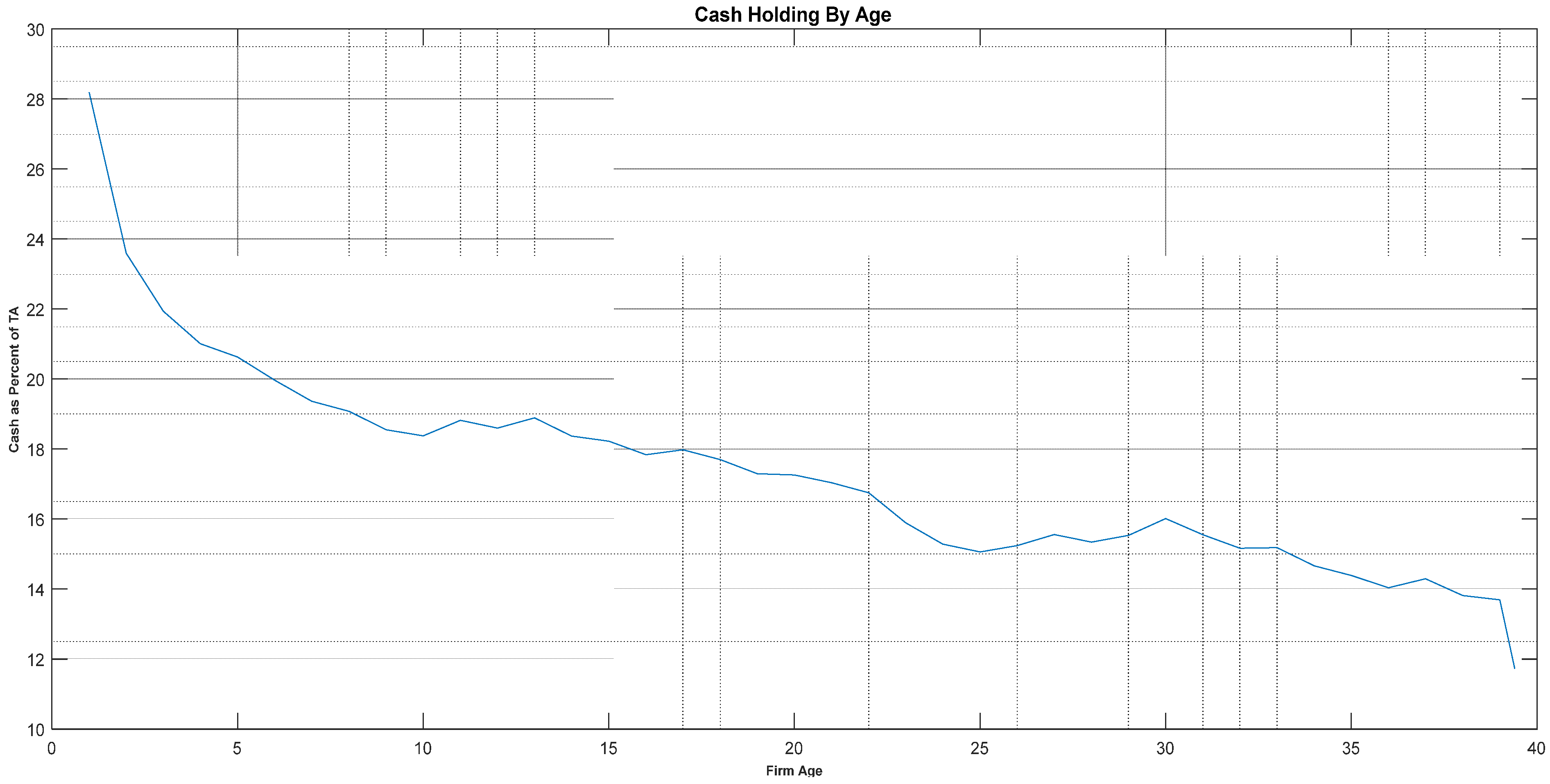
As depicted in Figure 2, we observed a negative relationship between the firm’s age and the level of cash holdings. Therefore, we also examined whether our macroeconomic variables have a similar impact on cash holding across firms of different sizes as measured by total assets. We divided our sample into four groups based on age and found that variables for macroeconomic conditions and uncertainties have an impact on the level of cash holdings irrespective of the firm’s age. Further, to examine the cross-sectional impact of macroeconomic variables on firms’ cash holdings, we also divided our samples into growth firms and value firms based on their market to book ratios. The real GDP growth rate and financial uncertainty have no impact on the firm’s cash holdings, but the other macroeconomic variables affect cash holdings the same in both groups. However, the ADS index and market factor show the impact differently on the cash holdings. The robustness test with growth vs. value firms can also conclude that macroeconomic variables have an impact on the level of cash holdings irrespective of the firm’s growth feature.

2. Related Literature

A theoretical framework that lays the groundwork for cash holdings consists of but is not limited to trade-off theory, the pecking order theory, and agency problems. According to the trade-off theory, firms decide to hold or change the level of cash holdings based on the marginal benefit and cost of holding cash. Based on the transaction cost motive in the trade-off theory, firms can decrease or minimize the transaction costs by raising external funds or liquidating their assets by holding a certain level of cash holdings (Dittmar et al. 2003). Opler et al. (1999) and Han and Qiu (2007) found supportive evidence for the trade-off theory, claiming that firms tend to hold cash to protect against costly adverse economic conditions. Opler et al. (1999), and Saunders and Steffen (2011) found debt is preferred over cash holdings for financing investment opportunities. Despite the marginal benefit of holding cash, Jensen (1986) claimed that cash holdings can cause agency costs. When firms hold a higher level of cash holdings, they will not ask for external capital and, therefore, can be away from the market monitoring, which could lead to a situation where the top management will pursue their interest rather than the shareholders’ interest. Chen et al. (2012) and Nikolov and Whited (2014) concluded that the agency perspective is responsible for the changes in cash holdings. According to Opler et al. (1999), the level of cash holdings depends on the firm’s decision on the investment and financing options. If a firm’s operating cash flows and cash holdings cannot cover payments and expenses for financing investments and debts, they require additional financing, which requires a higher rate of return. Therefore, the level of cash holdings is determined by the operating cash flows and expenses on the investment and financing options, which is called the pecking order theory. There has been substantial research to identify the relevant firm-specific variables to explain the change in cash holdings. Reflecting on the trade-off theory and the agency problem, Ferreira and Vilela (2004), Wasiuzzaman (2014), and Uyar and Kuzey (2014) applied the dividend payout, leverage, liquidity, and firm size to examine the cash holdings outlook. To study the pecking order theory for cash holdings, Ferreira and Vilela (2004) and Dittmar et al. (2003) employed R&D for investment activities, leverage, and operating cash flows. Following those previous studies, this paper introduces variables for the firm size, investment opportunities, leverage, profitability, liquidity, capital expenditure, dividend, and cash flow as firm-specific variables to explain the level of cash holdings. Under the precautionary motive, firms tend to accumulate cash holdings to finance their projects and investments if other financing options are not available. Bates et al. (2009) claimed that firms enhance their cash level to avoid the probability of higher costs of external financing.

Graham and Leary (2018) suggested that macroeconomic variables may be good candidates to explain the changes in cash holdings when firm characteristics do not have sufficient explanatory power. The macroeconomic environment is relevant to a firm’s cash-holding decision based on both transaction and precautionary motives. The transaction motive implies that firms would prefer holding cash as the internal source of capital to external sources, especially when the external sources become expensive due to poor economic conditions (Opler et al. 1999; Almeida et al. 2004; Han and Qiu 2007). The precautionary motive states that companies with more investment and growth opportunities hold more cash to hedge against very costly adverse shocks in cash flows (Faulkender and Wang 2006; Pinkowitz et al. 2006; Denis and Sibilkov 2010). Lins et al. (2010) distinguished corporate liquidity into the two parts of cash and lines of credit and found that lines of credit are related to a corporate’s need for external financing to fund investment opportunities, while cash is related to buffering against future cash shortage. Risk-averse management would behave more cautiously and prefer more cash holdings when it is less confident in future macroeconomic conditions and when it expects greater volatility in future cash flows and greater difficulty in accessing capital markets1.

The precautionary motive is also directly related to the dynamics of cash holdings over time via firms’ exposure to economic uncertainty. Recognition of this connection has elicited more recent research that incorporates economic uncertainties as to the other primary determinant of the firm’s cash holdings. Baum et al. (2006) concluded that when macroeconomic conditions are more volatile, managers will display more conservative behavior by increasing the liquidity level of the firm because they cannot predict future cash flow. Hackbarth et al. (2006) argued that the operating cash flows of the leveraged firm depend on the firm-specific shocks and the aggregate shocks that reflect the state of the economy. Gao et al. (2017) asserted that firm-level heterogeneous risks due to economic factors should be disaggregated into systematic risk and idiosyncratic risk and argued that uncertainties in macroeconomic factors should be considered in examining the change in cash holdings. Foley et al. (2007) and Acharya et al. (2013) found that aggregate-level uncertainties, such as changes in tax policy and frictions in a financial system, cause a change in firms’ cash holdings.

Our premise is that a major component of cash holdings is the firm’s exposure to macroeconomic conditions. This paper’s major contribution is to advance the analyses of cash holdings in the following manners. First, based on the premise that both time-series and cross-sectional variations in macroeconomic conditions would induce the change in cash holdings, this paper advances the growing literature on the level of cash holdings by incorporating the impact of various time-varying macroeconomic factors, following Graham and Leary (2018). To understand the upward trend in the level of cash holdings over multiple decades, prior literature has exploited unique firm-specific characteristics such as profitability, liquidity, and leverage (Opler et al. 1999; Dittmar et al. 2003; Harford et al. 2008; Denis and Sibilkov 2010; Subramaniam et al. 2011; Brisker et al. 2013; Qiu and Wan 2015; Chen et al. 2015; Tahir et al. 2016; Bates et al. 2018; Liu et al. 2021). However, prior literature has not explicitly documented the other potential determinants to the level of cash holdings. This research fills this gap by identifying and emphasizing that variables for macroeconomic conditions and uncertainty may be ingenious determinants of the level of cash holdings by applying variables for macroeconomic conditions and uncertainty in the theoretical frameworks of trade-off theory, precautionary motive, and transaction motive and by empirically proving their significance.

Second, this research sheds new light on how and how much variables for macroeconomic conditions and uncertainty influence the level of cash holdings. Tahir et al. (2016) concluded that previous research with the firm-specific variables provides mixed results in explaining the impact on the level of cash holdings. Graham and Leary (2018) found that firms’ characteristics have insufficient explanatory power to explain the changes in cash holdings. Introducing two sets of variables for macroeconomic conditions and uncertainty will improve the explanatory power to understand the change in the level of cash holdings. Through the presented models with three sets of variables presented in this paper, firms will be able to achieve the appropriate or optimal level of cash holdings.

Following Section 1 and Section 2, Section 3 will discuss the development of the hypotheses to test, and later in Section 4, data are described with all statistical and econometric methodology. Section 5 presents the results of each empirical test of a pooled model and a fixed model along with the robustness test with the different firm’s ages, the value vs. growth feature, and the endogeneity issue. In Section 6, this paper concludes. Appendix A is provided for detailed information on the variables.

3. Hypotheses

As Opler et al. (1999) and Han and Qiu (2007) asserted, the trade-off model of cash holdings entails that a firm’s optimal cash holdings are determined by the trade-off between the marginal costs and benefits of the cash holdings. The marginal costs of cash holdings are the combination of the opportunity cost of the capital invested in liquid assets and the agency cost stemming from holding excess cash by managers. Dittmar et al. (2003) stated that firms consider the marginal benefits and costs of the cash holdings to maximize the shareholders’ wealth. The marginal benefits rise from a decrease in transaction costs related to external funding (transaction motive) and take advantage of unanticipated investment opportunities (precautionary motive). In other words, cash holdings allow firms to save transaction costs for raising funds and to outfight the higher opportunity cost due to the lower level of cash, according to the transaction motive (Dittmar et al. 2003; Almeida et al. 2004; Han and Qiu 2007; Graham and Leary 2018). Under the precautionary motive, firms accumulate cash holdings to absorb economic shocks and to finance investment projects if other financing options are not available due to the economic shock or if firms are under financial distress (Ozkan and Ozkan 2004; Faulkender and Wang 2006; Pinkowitz et al. 2006; Bates et al. 2009). Both the costs and benefits of cash holdings are affected by firm-specific variables. According to the trade-off model, the cash holdings appear to have an impact on firm-specific variables such as leverage and firm size. Opler et al. (1999), Ferreira and Vilela (2004), Uyar and Kuzey (2014), and Wasiuzzaman (2014) incorporated dividend payout, leverage, firm size, liquidity, and risk to empirically test the trade-off theory for the firm’s cash holdings perspective and confirm the significance of those determinants. Another large volume of empirical studies employed the pecking order theory to explain the behavior of the cash holdings by incorporating firm-specific proxies of firm profitability, leverage, cash flow, and firm size and found evidence of their significance (Ferreira and Vilela 2004; Uyar and Kuzey 2014; Al-Najjar and Belghitar 2011).

Both the costs and benefits of cash holdings are affected by macroeconomic variables as well as firm-specific variables. The rise in the inflation rate and therefore the nominal interest rate, for example, would increase the opportunity cost of the capital invested in liquid assets and at the same time affect the transaction costs of raising capital from external sources. Therefore, according to the trade-off model, firms would tend to have more cash holdings when macroeconomic conditions are worse or when macroeconomic uncertainties increase due to the trade-off model. Graham and Leary (2018) suggested that the macroeconomic environment is relevant to a firm’s cash-holding decision based on both transaction and precautionary motives. Irvine and Pontiff (2009) noted that cash holdings are more valuable when the product market condition gets worse.

Julio and Yook (2012) claimed that aggregate uncertainty has an impact on a firm’s investment decision, and Gao et al. (2017) found a relationship between systematic uncertainty and the level of cash holdings. Under unexpected financial distress and economic uncertainty, firms may not be able to find the proper channel for external capital and, therefore, are expected to use the cash reserves immediately, as Neamtiu et al. (2014) noted. Stated formally, we hypothesize the following:

Hypothesis 1.

Macroeconomic variables will have a significant impact on the level of cash holdings.

i. 

Stability in economic condition (real GDP growth) and profitability (corporate profit) are expected to show a positive impact on the level of cash holdings.

ii. 

Inflation, a condition in the debt market (bond yield), and business condition (ADS index) are expected to show a negative impact on the level of cash holdings.

Hypothesis 2.

Macroeconomic uncertainties will display an adverse impact on the level of cash holdings through the operation channel and the financing channel.

i. 

Real GDP volatility is expected to show a positive impact on the level of cash holdings through the operation channel.

ii. 

Financial uncertainty and financial market factor are expected to show a negative impact on the level of cash holdings through the financing channel.

Fluctuations in economic conditions may cause a change in the business environment for firms, and therefore, they should adjust the level of cash holdings to cope with such fluctuations, as Anand et al. (2018) claimed. For example, under depressed economic conditions, firms may experience underperformance in sales and profit, resulting in a constant or decreasing level of cash holdings. Our measures of macroeconomic conditions impacting the changes in the firm-level cash holdings are real GDP growth rate (RGDP Growth), inflation (Inflation), corporate profit to GDP ratio (Corp. Prof/GDP), corporate bond yield (Corp. Bond Y), and the Aruoba–Diebold–Scotti index (ADS Index). The real GDP growth rate can show the expected conditions of the economy in the future that cannot be explained by firm-specific variables. We expect the real GDP growth rate to be positively related to the level of cash holdings because firms will have a lower cost of external financing and fewer financing constraints and, therefore, can accumulate more cash holdings, based on the trade-off theory, when the real GDP growth rate tends to increase. Inflation may have an impact on the level of cash holdings that is different from the real GDP growth rate. External financing can be more expensive when inflation and nominal interest rate are expected to rise. As Weidemann (2018) stated, firms tend to reduce the level of cash holdings when external financing becomes expensive, and cash holdings become costly, based on the trade-off theory. Firms would rather be better off with the investment in interest-bearing assets than holding cash and cash equivalents. Therefore, the higher the inflation expected, the fewer firms are incentivized to keep the level of cash holdings. Poor performance in profitability, represented by the corporate-profit-to-GDP ratio, can result in a situation where firms have insufficient liquidity to satisfy their liabilities. Therefore, firms need to consume cash and cash equivalents to do so. On the contrary, high profitability can supply enough liquidity to cover the liabilities and raise the level of cash holdings. We expect a positive association between the level of cash holdings and the corporate profit to GDP. The ADS index tracks the real business conditions with the underlying inputs of economic indicators such as payroll, industrial production, real GDP, personal income, and manufacturing and trade sales. The average value of the ADS index is 0. A bigger positive value means a better-than-average macroeconomic condition, and a negative value means a worse-than-average condition. Therefore, the ADS index is expected to have a negative association with cash holdings, as firms will be incentivized to collect more cash holdings when the macroeconomic condition seems worse.

The corporate bond yield can influence the level of cash holdings through the interest rate channel. Cash holdings become costly when inflation and nominal interest rate are expected to rise (Chen et al. 2012). As corporate bond YTM tends to rise when the interest rate goes up, our measure of corporate bond yield, the average YTM on Aaa- and Baa-rated bonds, will go up, and thus, the level of cash holdings is expected to decrease. The relationship between the corporate bond yield and the level of cash holdings can also be explained by the bond yield spread. The bond yield spread between bonds with different terms (long term vs. short term) and between bonds with different yields will be wider as the interest rate rises, as a long-term bond and a high-yield bond will be more exposed to the change in the interest rate, which indicates a stable economic condition in the future. Consequently, firms will have fewer preventive and precautionary incentives to increase the level of cash holdings.

Baum et al. (2006) asserted that firms can predict the accurate level of cash holdings when the macroeconomic conditions are stable. However, firms may increase the level of cash holdings on precautionary and preventive motivation when firms perceive uncertainty in the macroeconomic conditions. Uncertainty can influence cash holdings through the operation channel and the financing channel. Firms need operating cash flows to meet investment opportunities. Uncertainty in the macroeconomic conditions may disturb firms from predicting the accurate operating cash flows for investments in the future. Thus, firms will need to prepare a higher level of cash holdings when perceiving the uncertainty in the macroeconomic conditions, which will be more extensive if the opportunity cost of investment opportunities is high, and the cost of external financing is high. Our measure of the uncertainty through the operation channel is the conditional volatility of the real GDP growth rate (RGDP CV). The conditional volatility of the real GDP growth rate is measured by the GARCH model and represents the unexpected volatility of the real GDP. RGDP CV is expected to negatively influence the firm’s ability to predict accurate operating cash flows and thus will cause the level of cash holdings to increase. The financing channel means that uncertainty in the macroeconomic conditions affects the level of cash holdings through the change in the cost of external financing. Ferreira and Vilela (2004) claimed that macroeconomic conditions can be stabilized through the financial sector from an interest-rate-induced shock. Uncertainty in the macroeconomic conditions may increase the volatility in the cost of external financing, so firms may need to pay more for the external source of funds. To hedge against the expensive cost of external financing and uncertainty, firms will build an additional level of cash holdings. Uncertainty in the macroeconomic conditions, therefore, is expected to positively affect the level of cash holdings. Our measures of macroeconomic uncertainty in the financing channel are a 12-months-ahead forecast of financial uncertainty (FF Uncertainty) and market risk premium in the financial market (FF Mkt Factor). Both measures are designated to capture the uncertainty shock from the macroeconomic conditions through the financial market and, therefore, are expected to increase the level of cash holdings.

4. Data and Methodology

Our firm-specific variables for publicly traded firms were obtained from Standard and Poor’s annual Compustat database. Our sample spans from 1971 to 2019. We excluded all utilities and financial firms (SIC codes between 6000–6999 and 4900–4999) because utility firms are subject to regulatory oversight, and financial firms hold cash to maintain reserve requirements. We excluded firms with less than three years of observation because we used the lag of the dependent variable. We also excluded firms with negative sales or negative total assets. Our final sample consists of 19,223 unique firms with 213,663 firm-year observations. All continuous variables were winsorized at the 1% and 99 percent levels. Data for macroeconomic variables were collected from various sources (see Appendix A for data sources).

If CashRatio_it is the cash holdings of ith firm at time t, the cash holdings can be represented by the following panel data regression model:

$$\begin{array}{c}CashRati{o}_{it}=\lambda CashRati{o}_{i,t-1}+\beta {\mathit{C}\mathit{o}\mathit{n}\mathit{t}\mathit{V}\mathit{a}\mathit{r}\mathit{s}}_{it}+\gamma {\mathit{M}\mathit{a}\mathit{c}\mathit{r}\mathit{o}\mathit{V}\mathit{a}\mathit{r}\mathit{s}}_{it}+{\alpha }_i+{\theta }_i+{\mathit{u}}_{\mathit{i}\mathit{t}}\\ i=1, 2, 3,\cdots ,N; t=1, 2, 3,\cdots ,T\end{array}$$

(1)

where cash ratio stands for the ratio of firm-level cash and marketable securities to total assets, ContVars is a matrix of control variables, MacroVars is a matrix of macroeconomic variables, ${\alpha }_i$ is an unobservable firm-specific effect, ${\theta }_i$ is an unobservable industry-specific effect, λ is a scalar coefficient of the lagged cash ratio, $\beta$ is a coefficient vector of control variables, $\gamma$ is a coefficient vector of macroeconomic variables, and $u_{it}$ is an idiosyncratic error term.

Following Bates et al. (2009), we have ten control variables. They include the one-year lag value of corporate cash to assets ratio (L. Cash Ratio), market to book ratio (MB Ratio), firm size (Firm Size), cash flow to assets ratio (CF Ratio), networking to capital assets (NWC Ratio), capital expenditures to assets (Capex Ratio), leverage (Leverage Ratio), R&D to sales (RD/Sales ratio), acquisition to assets (Acq. Ratio), and dividend payout dummy (Dividend). The definitions of these control variables as well as eight other macroeconomic variables are provided in Appendix A. Using these control variables, our baseline model with the firm- and industry-fixed effect is

$$\begin{array}{l}CashRati{o}_{it}=\lambda CashRati{o}_{i,t-1}+{\beta }_{1}MB Rati{o}_{it}+{\beta }_{2}Firm Siz{e}_{it}+{\beta }_3 CF Rati{o}_{it}+\\ {\beta }_{4}NWC Rati{o}_{it}+{\beta }_{5}Capex Rati{o}_{it}+{\beta }_{6}Leverage Rati{o}_{it}+{\beta }_7\frac{RD}{Sales}rati{o}_{it}+\\ {\beta }_{8}Acq. Rati{o}_{it}+{\beta }_{9}Dividen{d}_{it}+{\alpha }_i+{\theta }_i+u_{it}\end{array}$$

(2)

To measure the impact of macroeconomic variables on cash holdings, we augmented model 2 with a different set of macroeconomic variables that capture the state of the macroeconomic condition and uncertainty. Five macroeconomic variables measure the state of the macroeconomic condition. They include Aruoba–Diebold–Scotti business conditions index (ADS Index), real GDP growth rate, inflation, corporate profit, and corporate bond yield. The ADS index tracks real business conditions by combining high-frequency and low-frequency data. The expected value of the ADS index is zero. Bigger positive values of the ADS index indicate better-than-average conditions, and more negative values indicate worse-than-average conditions. The other two macroeconomic variables are straightforward to measure and include real GDP growth (RGDP Growth) and inflation (Inflation). Similar to the ADS index, RGDP growth will positively impact corporate liquidity, whereas inflation harms cash holdings. The nonfinancial corporate profits after tax without inventory valuation adjustment and capital consumption adjustment as a percentage of gross domestic product (Corp. Prof/GDP) is used to measure the impact of aggregate corporate financial performance on firm-level cash holdings. Similarly, we used the average of Moody’s seasoned Aaa and Baa corporate bond yields (Corp. Bond Y), defined as (annual yield on Aaa rated bond + annual yield on Baa rated bond)/2, to capture the opportunity cost of holding cash and examine its impact on cash holdings After augmenting model 2 by these macroeconomic condition variables, our next model takes the following form:

$$\begin{array}{l}CashRati{o}_{it}=\lambda CashRati{o}_{i,t-1}+\beta ContVar{s}_{it}+{\gamma }_1 ADS Inde{x}_{it}+\\ {\gamma }_2 RGDP Growt{h}_{it}+{\gamma }_3 CP{I}_{it}+{\gamma }_4 Corp. Prof/GD{P}_{it}+{\gamma }_5 Corp. Bond Y_{it}+{\alpha }_i+{\theta }_i+u_{it}\end{array}$$

(3)

The other three macroeconomic variables that capture the macroeconomic uncertainty are the conditional variance of real gross domestic product (RGDP CV), a measure of financial uncertainty, and the Fama–French market factor. The time-varying conditional variance of real GDP growth rate (RGDP CV) is measured using AR (1)-GARCH (1,1) model. The mean and variance equations of real GDP growth (RGDPg) are specified as follows:

$$RGDP{g}_t=\phi RGDP{g}_{t-1}+{\epsilon }_t where {\epsilon }_t~N\left(0,h_t\right)$$

(4)

$$h_t=\omega +{\phi }_1 h_{t-1}+{\phi }_2{\epsilon }_{t-1}^2$$

(5)

Equations (4) and (5) are jointly estimated with the maximum likelihood method. The conditional standard deviation $\sqrt{h_t}$ estimated using Equations (4) and (5) is used as a measure of macroeconomic uncertainty. The impact of variability on corporate liquidity could be positive or negative.

The 12-months-ahead measure of financial uncertainty was taken from Jurado et al. (2015). The stock market volatility to proxy for financial uncertainty is expected to have a negative impact on corporate cash holdings. The Fama–French market factor measures the overall market risk premium and is expected to positively impact corporate cash holdings. With all the macroeconomic variables, our complete model takes the following form:

$$\begin{array}{l}CashRati{o}_{it}=\lambda CashRati{o}_{i,t-1}+\beta ContVar{s}_{it}+{\gamma }_1 ADS Inde{x}_{it}+\\ {\gamma }_2 RGDP Growt{h}_{it}+{\gamma }_3 CP{I}_{it}+{\gamma }_4 Corp.{\frac{Prof}{GDP}}_{it}+{\gamma }_5 Corp. Bond Y_{it}+{\gamma }_6 RGDP C{V}_{it}+\\ {\gamma }_7 Fin. Uncertaint{y}_{it}+{\gamma }_8 FF Mkt Facto{r}_{it}+{\alpha }_i+{\theta }_i+u_{it}\end{array}$$

(6)

Our unbalanced panel models represented by Equations (2), (3) and (6) are estimated using a pooled OLS estimator and fixed-effects estimator with cluster-robust standard errors. Positive coefficients on the macro variables mean that they positively impact the cash ratio. In contrast, negative coefficients indicate that they have a negative impact on the cash ratio. We tested these hypotheses using pooled and fixed-effects regression for the whole and subsamples using t-test and F statistics. To examine the impact of all macroeconomic variables on the cash holdings, we used Wald tests to test joint hypotheses, equating all coefficients on the macroeconomic variables to zero.

5. Results

5.1. Summary Statistics

Table 1. Descriptive Statistics.

	N	Mean	SD	Min	Q1	Median	Q3	Max
Cash Ratio	213,663	16.16	20.13	0	2.53	7.84	21.52	89.07
MB Ratio	213,663	226.79	314.67	51.79	101.03	136.84	216.74	2452.88
Firm Size	213,663	4.72	2.39	−0.83	3.04	4.59	6.35	10.55
CF Ratio	213,663	−6.47	48.09	−350.02	−1.68	5.63	9.91	27.17
NWC Ratio	213,663	2.13	47.23	−344.13	−4.57	6.72	22.33	56.47
Capex Ratio	213,663	6.85	7.70	0	1.99	4.37	8.63	42.87
Lev. Ratio	213,663	28.16	32.76	0	6.5	22.18	38.27	231.35
RD/Sales	213,663	22.97	119.50	0	0	0	3.84	1022.51
Acq. Ratio	213,663	1.87	5.55	−0.37	0	0	0.17	34.04
Dividend	213,663	0.35	0.48	0	0	0	1	1
ADS Index	213,663	−0.12	0.92	−3.68	−0.39	−0.02	0.41	1.64
RGDP Growth	213,663	2.73	2.08	−3.3	1.61	2.79	4.17	8.32
Inflation	213,663	3.48	2.53	0.01	2.02	2.93	3.97	12.51
Corp. Prof/GDP	213,663	7.11	2.08	3.92	5.16	6.54	9.22	11.7
Corp. Bond Y	213,663	7.74	2.66	3.44	5.82	7.41	9.23	15.39
RGDP CV	213,663	5.2	2.18	2.97	3.6	4.35	6.24	11.48
Fin. Uncertainty	213,663	0.98	0.05	0.91	0.94	0.98	1.02	1.11
FF Mkt Factor	213,663	7.95	17.57	−38.34	−3.87	11.55	20.57	35.2

This table presents the descriptive statistics for all variables. The sample consists of 19,223 unique firms from Compustat’s annual files and spans from 1971 to 2019. All firm-specific variables are scaled by total assets and winsorized at the top and bottom at the 1% level. The Cash Ratio is the ratio of cash and marketable securities to total assets. Similarly, MB Ratio is computed as the ratio of the market value of total assets to the book value of total assets. The natural logarithm of the book value of total assets is defined as Firm Size. CF Ratio is cash flows to total asset ratio, defined as the operating income before depreciation minus interest expense, taxes, and dividend scaled by total assets. NWC Ratio is net working capital to total assets, computed as the current assets excluding cash and marketable securities minus current liabilities and divided by the book value of total assets. Capex Ratio is the ratio of capital expenditure to book value of total assets. Lev. Ratio is the leverage ratio computed as the ratio of short-term and long-term debt to total assets. RD/Sales is research and development expense as a percent of total sales. Acq. Ratio is the acquisition ratio calculated as the ratio of total acquisition to total assets or 0 if missing. Dividend is a dummy variable that is 1 if the dividend is positive and zero otherwise. ADS Index is the Aruoba–Diebold–Scotti business conditions index. RGDP Growth is the change in the real gross domestic product (GDP). Inflation is the percentage change in the consumer price index. Corp. Prof/GDP is computed as the corporate profit to GDP ratio. Corp. Bond Y is an equally weighted average yield on Aaa- and Baa-rated bonds. RGDP CV is conditional volatility of real GDP growth rate. Fin. Uncertainty is a 12-months-ahead forecast of financial uncertainty. FF. Mkt Factor is the Fama–French market factor. See Appendix A for detailed variable definitions and their computation.

presents the descriptive statistics for the firm-specific control variables and variables for macroeconomic conditions. The average cash ratio is 16.16%, and the median is 7.84%. The MB ratio for the growth prospect is 226.79, indicating the high growth potential for all firms in the U.S. economy. The average size of a firm is 4.72, and the firm’s profitability (cash flow to assets) is not as good at −6.47%. A firm has 2.13% in liquid assets on average, has 28.16% debt on its balance sheet, and brings about 6.85% of capital expenditure. Research and development incur 22.97% of sales, and acquisition is low at 1.87%.

The average ADS index is −0.12, suggesting that the macroeconomic condition is worse than the average condition in the overall sample years. Real GDP has been growing by 2.73%, and the average inflation rate is 3.48%. Firms showed 7.11% of financial performance, and the average bond yield was 7.74%. Over the sample period, macroeconomic uncertainty increased by 5.2%, and financial uncertainty was low at 0.98%. The average market risk premium is 7.95%.

Table 2. Pearson Correlation Coefficients.

Variables	(1)	(2)	(3)	(4)	(5)	(6)	(7)	(8)	(9)	(10)	(11)	(12)	(13)	(14)	(15)	(16)	(17)	(18)
(1) Cash Ratio	1.00
(2) MB Ratio	0.29 ***	1.00
(3) Firm Size	−0.19 ***	−0.29 ***	1.00
(4) CF Ratio	−0.22 ***	−0.62 ***	0.39 ***	1.00
(5) NWC Ratio	−0.14 ***	−0.53 ***	0.18 ***	0.64 ***	1.00
(6) Capex Ratio	−0.16 ***	−0.01 ***	0.02 ***	0.07 ***	−0.05 ***	1.00
(7) Lev. Ratio	−0.26 ***	0.26 ***	−0.06 ***	−0.39 ***	−0.54 ***	0.02 ***	1.00
(8) RD/Sales	0.39 ***	0.27 ***	−0.14 ***	−0.39 ***	−0.17 ***	−0.07 ***	0.01 **	1.00
(9) Acq. Ratio	−0.09 ***	−0.03 ***	0.12 ***	0.06 ***	0.01 ***	−0.06 ***	0.05 ***	−0.04 ***	1.00
(10) Dividend	−0.21 ***	−0.17 ***	0.41 ***	0.21 ***	0.18 ***	0.03 ***	−0.10 ***	−0.14 ***	0.01 ***	1.00
(11) ADS Index	0.00	0.03 ***	−0.03 ***	0.02 ***	0.03 ***	−0.01 ***	−0.02 ***	−0.01 ***	0.01 ***	0.00	1.00
(12) RGDP Growth	−0.02 ***	0.00	−0.08 ***	0.04 ***	0.07 ***	0.02 ***	−0.02 ***	−0.03 ***	0.01 ***	0.01 ***	0.81 ***	1.00
(13) Inflation	−0.14 ***	−0.13 ***	−0.17 ***	0.11 ***	0.18 ***	0.11 ***	−0.02 ***	−0.08 ***	−0.07 ***	0.19 ***	−0.15 ***	−0.11 ***	1.00
(14) Corp. Prof/GDP	0.11 ***	0.08 ***	0.23 ***	−0.08 ***	−0.15 ***	−0.11 ***	0.01 ***	0.06 ***	0.01 ***	−0.00 **	0.02 ***	−0.14 ***	−0.15 ***	1.00
(15) Corp. Bond Y	−0.15 ***	−0.13 ***	−0.26 ***	0.12 ***	0.20 ***	0.16 ***	−0.03 ***	−0.09 ***	−0.06 ***	0.13 ***	−0.02 ***	0.08 ***	0.63 ***	−0.67 ***	1.00
(16) RGDP CV	−0.10 ***	−0.12 ***	−0.15 ***	0.09 ***	0.15 ***	0.10 ***	−0.03 ***	−0.08 ***	−0.06 ***	0.16 ***	0.22 ***	0.30 ***	0.35 ***	−0.21 ***	0.55 ***	1.00
(17) Fin. Uncertainty	−0.04 ***	−0.05 ***	−0.03 ***	0.00	0.02 ***	0.02 ***	0.03 ***	−0.01 ***	−0.01 ***	0.02 ***	−0.45 ***	−0.32 ***	0.19 ***	−0.28 ***	0.16 ***	−0.02 ***	1.00
(18) FF Mkt Factor	0.02 ***	0.06 ***	0.02 ***	0.01 ***	−0.01 ***	−0.03 ***	−0.01 ***	0.00	0.01 ***	−0.01 ***	0.59 ***	0.51 ***	−0.18 ***	0.14 ***	−0.15 ***	0.05 ***	−0.44 ***	1.00

This table presents the correlation between the cash ratio and all firm-specific and macroeconomic variables. The 1% and 5% significance levels are denoted with *** and **, respectively. The Cash Ratio is the ratio of cash and marketable securities to total assets. Similarly, MB Ratio is computed as the ratio of the market value of total assets to the book value of total assets. The natural logarithm of the book value of total assets is defined as Firm Size. CF Ratio is cash flows to total asset ratio, defined as the operating income before depreciation minus interest expense, taxes, and dividend scaled by total assets. NWC Ratio is net working capital to total assets, computed as the current assets excluding cash and marketable securities minus current liabilities divided by the book value of total assets. Capex Ratio is the ratio of capital expenditure to book value of total assets. Lev. Ratio is the leverage ratio computed as the ratio of short-term and long-term debt to total assets. RD/Sales is research and development expense as a percent of total sales. Acq. Ratio is the acquisition ratio calculated as the ratio of total acquisition to total assets or 0 if missing. Dividend is a dummy variable that is 1 if the dividend is positive and zero otherwise. ADS Index is Aruoba–Diebold–Scotti business conditions index. RGDP Growth is the change in the real gross domestic product (GDP). Inflation is the percentage change in the consumer price index. Corp. Prof/GDP is computed as the corporate profit to GDP ratio. Corp. Bond Y is an equally weighted average yield on Aaa- and Baa-rated bonds. RGDP CV is conditional volatility of real GDP growth rate. Fin. Uncertainty is a 12-months-ahead forecast of financial uncertainty. FF. Mkt Factor is the Fama-French market factor. See Appendix A for detailed variable definitions and their computation.

shows correlations among variables. However, there is no outstanding multicollinearity problem among firm-specific control variables except between NWC Ratio and CF Ratio. However, both firm-specific variables were applied to the empirical test by previous research, such as that of Bates et al. (2009) and Graham and Leary (2018), so we follow them. Over the presented correlations, we found a high correlation between RGDP Growth and ADS Index.

It may not be believed that any multicollinearity problem is incurred because the ADS index is a comprehensive index not only with real GDP but also factors in trade, industrial production, joblessness, and consumption. Corp. Bond Y presents high correlations with inflation and Corp. Profit/GDP. However, according to the definitions of those variables and how they are derived, we may believe that those would not cause the multicollinearity issue undermining the statistical significance. All variables are shown to have an association with the level of cash holdings.

5.2. Impact of Macroeconomic Conditions on the Level of Cash Holdings, Pooled Model

Table 3. Pooled Estimates.

	Model 1		Model 2		Model 3
	Estimate	p-Value	Estimate	p-Value	Estimate	p-Value
L. Cash Ratio	0.6722 ***	(0.00)	0.6717 ***	(0.00)	0.6719 ***	(0.00)
MB Ratio	0.0067 ***	(0.00)	0.0067 ***	(0.00)	0.0066 ***	(0.00)
Firm Size	−0.1114 ***	(0.00)	−0.1231 ***	(0.00)	−0.1297 ***	(0.00)
CF Ratio	0.0394 ***	(0.00)	0.0394 ***	(0.00)	0.0393 ***	(0.00)
NWC Ratio	−0.0525 ***	(0.00)	−0.0519 ***	(0.00)	−0.0518 ***	(0.00)
Capex Ratio	−0.2792 ***	(0.00)	−0.2792 ***	(0.00)	−0.2787 ***	(0.00)
Lev. Ratio	−0.1021 ***	(0.00)	−0.1014 ***	(0.00)	−0.1013 ***	(0.00)
RD/Sales	0.0191 ***	(0.00)	0.0192 ***	(0.00)	0.0192 ***	(0.00)
Acq. Ratio	−0.3460 ***	(0.00)	−0.3466 ***	(0.00)	−0.3469 ***	(0.00)
Dividend	−2.0102 ***	(0.00)	−1.9720 ***	(0.00)	−1.9399 ***	(0.00)
ADS Index			−0.0158	(0.69)	−0.1094 *	(0.01)
RGDP Growth			0.0555 **	(0.00)	0.0560 **	(0.00)
Inflation			−0.1845 ***	(0.00)	−0.1969 ***	(0.00)
Corp. Prof/GDP			0.2145 ***	(0.00)	0.2466 ***	(0.00)
Corp. Bond Y			0.2273 ***	(0.00)	0.2908 ***	(0.00)
RGDP CV					−0.0700 ***	(0.00)
Fin. Uncertainty					1.3916 *	(0.03)
FF Mkt Factor					0.0141 ***	(0.00)
Constant	10.4087 ***	(0.00)	10.4177 ***	(0.00)	5.8656 ***	(0.00)
F-Statistics			54.30	(0.00)	44.84	(0.00)
No. observations	213,663		213,663		213,663
Adj. R2	0.6698		0.6702		0.6703

This table presents the coefficient estimates and p-values in parentheses from pooled OLS regression using firm-level annual cash and short-term investment to total assets ratio as a dependent variable. The total number of firms in the sample is 19,223, and the sample period spans from 1971 to 2019. The Cash Ratio is the ratio of cash and marketable securities to total assets. Similarly, MB Ratio is computed as the ratio of the market value of total assets to the book value of total assets. The natural logarithm of the book value of total assets is defined as Firm Size. CF Ratio is cash flows to total asset ratio, defined as the operating income before depreciation minus interest expense, taxes, and dividend scaled by total assets. NWC Ratio is net working capital to total assets, computed as the current assets excluding cash and marketable securities minus current liabilities divided by the book value of total assets. Capex Ratio is the ratio of capital expenditure to book value of total assets. Lev. Ratio is the leverage ratio, computed as the ratio of short-term and long-term debt to total assets. RD/Sales is research and development expense as a percent of total sales. Acq. Ratio is the acquisition ratio, calculated as the ratio of total acquisition to total assets or 0 if missing. Dividend is a dummy variable, which is 1 if the dividend is positive and zero otherwise. ADS Index is the Aruoba–Diebold–Scotti business conditions index. RGDP Growth is the change in the real gross domestic product (GDP). Inflation is the percentage change in the consumer price index. Corp. Prof/GDP is computed as the corporate profit to GDP ratio. Corp. Bond Y is an equally weighted average yield on Aaa- and Baa-rated bonds. RGDP CV is conditional volatility of the real GDP growth rate. Fin. Uncertainty is 12-months-ahead forecast of financial uncertainty. FF. Mkt Factor is the Fama–French market factor. See Appendix A for detailed variable definitions and their computation. Model 1 is a baseline regression model with only control variables as explanatory variables. Model 2 extends model 1 by adding five macroeconomic variables that capture the state of macroeconomic conditions. Similarly, model 3 adds three more macroeconomic variables that capture macroeconomic uncertainty to model 2. The 1%, 5%, and 10% significance levels are denoted with ***, **, and *, respectively. See Appendix A for variable definitions and their computation.

shows the result of the pooled regression for the cash holdings on each variable for macroeconomic conditions and control variables. Pooled regression can usually be carried out on time-series data for different cross-sections. By applying the whole sample, pooled regression aims to show whether and how variables for macroeconomic conditions impact the level of cash holdings. Consistent with Gao et al. (2017) and Graham and Leary (2018), we introduced the firm-specific control variables as follows: lagging level of cash holdings (L. Cash Ratio), market to book ratio (MB Ratio), firm size (Firm Size), cash flows (CF Ratio), net working capital (NWC Ratio), capital expenditure (Capex Ratio), leverage condition (Lev. Ratio), R&D expenditure (RD/Sales), dividend payout ratio (Dividend), and acquisitions (Acq. Ratio). MB Ratio reflects the firm’s growth prospects, and a high MB Ratio indicates optimistic growth prospects, suggesting that firms may need to hold more cash holdings or liquid assets because the cost of credit or external financing for such a firm may be high, as claimed by Opler et al. (1999) Therefore, MB Ratio is expected to be positively related with the cash holdings. The general benefit of the cash holdings depends on whether and how much, if possible, firms can save transaction costs related to external financing and a firm’s access to the financial market, determined by the firm’s size, profitability, investment opportunities, the availability of liquidity substitutes, and leverage. As a firm get bigger, it may be less incentivized to hold cash, as it can have other types of liquidity substitutes. Profitability, measured by CF Ratio, is expected to have a positive relationship. The higher the net working capital for the liquidity substitute and the investment for the capital expenditure, the less chance to add the level of cash holdings. When firms have a high debt ratio, they should prepare a high volume of cash to meet the interest and principal payments for short- and long-term obligations. If firms have specific future uses in mind, such as R&D, firms will hold more cash holdings for such a known expenditure. Acquisition expenditure consumes cash holdings and other types of liquidity. Firms will be able to accumulate fewer cash holdings or need to consume the current level of cash holdings to make the dividend payout, and therefore, there is a negative association between dividend payout and the level of cash holdings.

In all three models, we found strong evidence that the lag of the cash ratio significantly and positively affects the current level of cash holdings. For example, in model 1, the coefficient of lag of the cash ratio is 0.6722, indicating that firms can accumulate 32.78% of their optimal level of cash holdings within one year.2 As expected, it is noticed that there is a change in adj. R-square, indicating that firms would be able to find the optimal level of cash holdings not only considering firm-specific factors but also macroeconomic conditions.

Model 1 in Table 3 shows the result of the base model with only the control variables. All control variables are statistically significant: this result is consistent with Gao et al. (2017) and Graham and Leary (2018). Control variables were found to be consistent with the hypotheses stated above. Positive signals and performance such as MB Ratio, CF Ratio, and RD/Sales increase the level of cash holdings because they represent the firm’s growth prospects, profitability, and optimistic prospects. In the meantime, expenditures such as NWC Ratio, Capex Ratio, Lev. Ratio, Dividend, and Acq. Ratio lead to a decrease or consumption of the cash holdings.

Test results with variables for macroeconomic conditions are shown for model 2 in Table 3. Firm-specific control variables are statistically significant and are still consistent even with the application of macroeconomic variables with the result in model 1. The real GDP growth rate shows a positive relationship with the level of cash holdings, as hypothesized. As the real GDP growth rate indicates a stable economic condition, firms face favorable financial constraints and a lower cost of external financing so that firms can keep more cash holdings. The results of checking the influence of inflation along with the real GDP growth rate are presented. The real GPD growth rate maintains its significance. and inflation shows a negative relationship. as expected. When inflation rises, external financing becomes costly, and firms would rather invest in interest-bearing assets than keep cash in the vault as the interest rate goes up. It was also checked if the firm’s profitability has an impact on the cash holdings, and we confirm that a firm’s profitability is another source for the cash holdings to rise.

To check how the macroeconomic environment derived from the debt market affects the level of cash holdings, the corporate bond yield needs to be applied in the regression. For that purpose, the average yield to maturity on Aaa- and Baa-rated bonds was applied and expected to have a negative relationship with the level of cash holdings through the interest rate and yield spread channels. Test results suggest that the rise in the average yield to maturity results in an increase in cash holdings, which may be explained by the refinancing risk in the bond market. Refinancing risk occurs when firms are not able to obtain the refinancing. When the yield to maturity rises, firms may find difficulty in refinancing, so cash holdings can assist firms to pay off debt and reduce the likelihood of insufficient liquidity (Gao et al. 2013). As expected, the ADS index has a negative association with cash holdings, as firms will be more incentivized to collect more cash holdings when the macroeconomic condition seems worse.

Uncertainty in macroeconomic conditions is considered to hinder the firm’s ability to predict the operating cash flows and accurate level of cash holdings. To determine the influence of uncertainty on the level of cash holdings, the three variables of conditional volatility of real GDP growth rate, forecast of financial uncertainty, and financial market premium were applied, and the test results are presented for model 3 along with control variables and variables for macroeconomic conditions. Not only variables for macroeconomic conditions but also those for uncertainty are confirmed as statistically significant, as expected. It is not usually possible for firms to increase cash holdings under a volatile macroeconomic situation in the future because under uncertain economic conditions measured by conditional volatility of the real GDP growth rate, illiquid conditions and financial distress may harden so that firms cannot raise external capital, and therefore, they should spend cash holdings. As an illustration of the economic significance, we multiplied the mean values for each macroeconomic variable by the regression coefficient and divided them by the mean value for the Cash Ratio. ADS Index accounts for 0.08%, RGDP Growth 0.95%, Inflation 4.24%, Corp. Prof/GDP 10.85%, and Corp. Bond Y 13.93%, showing that variables for macroeconomic conditions account for a total of 30.05%3 of the mean Cash Ratio. On average, 30.05% of the changes in the level of cash holdings are attributed to the macroeconomic condition. Similarly, we found that RGDP CV accounts for 2.25% of the mean Cash Ratio, Fin. Uncertainty 8.44%, and FF Mkt Factor 0.69%.

Conclusively, we can claim that firms should take macroeconomic conditions and uncertainty into consideration as well as firm-specific variables to determine the appropriate level of cash holdings because variables for macroeconomic conditions and uncertainties are economically significant, as they account for the total of 41.43% and are found to be statistically significant based on model 3 shown in Table 3. Our F-test statistics of the joint hypothesis of whether macroeconomic variables included in each model have a joint influence on cash holdings show that these macroeconomic variables have a significant impact on corporate cash holdings.

5.3. Impact of Macroeconomic Conditions on the Level of Cash Holdings, Fixed-Effect Model

To capture the full firm-level and industry-level fixed effects of firms’ behavior regarding cash holdings in response to various variables for macroeconomic conditions and uncertainty measures, we applied the fixed-effect model. The results are reported in

Table 4. Fixed-Effects Estimates.

	Model 1		Model 2		Model 3
	Estimate	p-Value	Estimate	p-Value	Estimate	p-Value
L. Cash Ratio	0.3601 ***	(0.00)	0.3600 ***	(0.00)	0.3599 ***	(0.00)
MB Ratio	0.0071 ***	(0.00)	0.0071 ***	(0.00)	0.0071 ***	(0.00)
Firm Size	−0.6535 ***	(0.00)	−0.6447 ***	(0.00)	−0.5305 ***	(0.00)
CF Ratio	0.0411 ***	(0.00)	0.0409 ***	(0.00)	0.0403 ***	(0.00)
NWC Ratio	−0.0504 ***	(0.00)	−0.0505 ***	(0.00)	−0.0513 ***	(0.00)
Capex Ratio	−0.2728 ***	(0.00)	−0.2717 ***	(0.00)	−0.2793 ***	(0.00)
Lev. Ratio	−0.1135 ***	(0.00)	−0.1133 ***	(0.00)	−0.1127 ***	(0.00)
RD/Sales	0.0142 ***	(0.00)	0.0142 ***	(0.00)	0.0141 ***	(0.00)
Acq. Ratio	−0.2737 ***	(0.00)	−0.2742 ***	(0.00)	−0.2747 ***	(0.00)
Dividend	0.4564 ***	(0.00)	0.4666 ***	(0.00)	0.3097 **	(0.00)
ADS Index			0.3598 ***	(0.00)	−0.0794 *	(0.05)
RGDP Growth			0.0071 ***	(0.00)	0.0524 **	(0.01)
Inflation			−0.5490 ***	(0.00)	−0.1550 ***	(0.00)
Corp. Prof/GDP			0.0405 ***	(0.00)	0.2102 ***	(0.00)
Corp. Bond Y			−0.0511 ***	(0.00)	0.3808 ***	(0.00)
RGDP CV					0.0563 **	(0.00)
Fin. Uncertainty					−1.6134 *	(0.02)
FF Mkt Factor					0.0074 ***	(0.00)
Constant	17.2974 ***	(0.00)	17.2786 ***	(0.00)	13.9812 ***	(0.00)
F Statistics			88.42	(0.00)	59.26	(0.00)
Firm FE	Yes		Yes		Yes
Industry FE	Yes		Yes		Yes
No. observations	213,663		213,663		213,663
Adj. R2	0.2401		0.2403		0.2424

This table presents the coefficient estimates and p-values in parentheses from fixed-effects regression. The total number of firms in the sample is 19,223, and the sample period spans from 1971 to 2019. The dependent variable in all regressions is the firm-level ratio of cash and marketable securities to the book value of total assets. The Cash Ratio is the ratio of cash and marketable securities to total assets. Similarly, MB Ratio is computed as the ratio of the market value of total assets to the book value of total assets. The natural logarithm of the book value of total assets is defined as Firm Size. CF Ratio is cash flows to total asset ratio, defined as the operating income before depreciation minus interest expense, taxes, and dividend scaled by total assets. NWC Ratio is net working capital to total assets, computed as the current assets excluding cash and marketable securities minus current liabilities divided by the book value of total assets. Capex Ratio is the ratio of capital expenditure to book value of total assets. Lev. Ratio is the leverage ratio, computed as the ratio of short-term and long-term debt to total assets. RD/Sales is research and development expense as a percent of total sales. Acq. Ratio is the acquisition ratio, calculated as the ratio of total acquisition to total assets or 0 if missing. Dividend is a dummy variable that is 1 if the dividend is positive and zero otherwise. ADS Index is the Aruoba–Diebold–Scotti business conditions index. RGDP Growth is the change in the real gross domestic product (GDP). Inflation is the percentage change in the consumer price index. Corp. Prof/GDP is computed as the corporate profit to GDP ratio. Corp. Bond Y is an equally weighted average yield on Aaa- and Baa-rated bonds. RGDP CV is conditional volatility of real GDP growth rate. Fin. Uncertainty is a 12-months-ahead forecast of financial uncertainty. FF. Mkt Factor is the Fama–French market factor. See Appendix A for detailed variable definitions and their computation. Model 1 is a baseline regression model with only control variables as explanatory variables. Model 2 extends model 1 by adding five macroeconomic variables that capture the state of macroeconomic conditions. Similarly, model 3 adds three more macroeconomic variables that capture macroeconomic uncertainty to model 2. The 1%, 5%, and 10% significance levels are denoted with ***, **, and *, respectively. See Appendix A for variable definitions and their computation.

. Under fixed effects, overall, firms tend to have a higher portion of their target cash holdings within a year measured by the lag of cash ratios. In all models, the coefficients for firm-specific variables remain quantitatively the same as those in pooled regression with the one exception of dividend payout. The fixed-effect model presents a positive relationship between the dividend payout and the level of cash holdings, suggesting that dividend-paying firms hold a higher level of cash holdings than non-dividend-paying firms to prevent a situation in which firms have insufficient cash holdings (Ozkan and Ozkan 2004).

In model 2, the coefficients for variables for macroeconomic conditions in the fixed-effect model seem to have the same effect on the level of cash holdings with two main exceptions. Within the whole firm-level observations, firms are expected to accumulate a higher volume of cash holdings when the economic condition seems worse than average and, therefore, to show a negative relationship between the level of cash holdings and the ADS index. However, the ADS index was found negatively related, indicating that, under the firm-fixed effect, firms would apply the ADS index to be the reference for the future so that they can increase the level of cash holdings when they find a worse-than-average economic condition by the ADS index. In pooled regression in Table 3, the Corp. Bond Y was found negatively related due to the refinancing risk. Firms tend to worry about the refinancing risk when they need to decide the appropriate level of cash holdings at the increase in the interest rate and at the wider bond yield spread. However, with the fixed effects, firms generally believe that the wider bond yield spread claims a stable economic condition, and therefore, they will have fewer incentives to increase the level of cash holdings.

In model 3, conditional volatility for the real GDP growth rate shows a positive relationship with the level of cash holdings. Through the operation and financing channels, it seems that uncertain economic conditions exacerbate a firm’s ability to predict the appropriate level of cash holdings, and thus, firms would stack up more cash holdings intentionally to supply sufficient financial sources and to avoid the expensive financing cost. Firms seem to pay attention to long-term financial uncertainty prediction in negatively gauging the accurate level of cash holdings.4 Under volatile macroeconomic conditions in the future, it may not be easy for firms to secure a certain level of cash holdings. Rather, they are asked to consume their cash holdings for projects that may not be funded by external sources due to the higher uncertainty in the financial markets, which is represented by Fin. Uncertainty.

Lastly, firms should check the expected macroeconomic situation in the future to determine if they need to increase the volume of cash holdings because the real GDP growth rate has a statistically positive significance on the level of cash holdings in all fixed-effect models. Consistent with the result in the pooled model, firms may not need to prepare a higher volume of cash holdings due to the better accessibility to the credit markets as they mature. However, firms may understand the impact of macroeconomic uncertainty differently in that each firm seems to take the operational uncertainty presented by RGDP CV negatively and the financial uncertainty presented by Fin. Uncertainty positively, but overall, firms with fixed effects take those two variables oppositely.

The F-statistics reported in Table 4 test whether the macroeconomic variables, taken as a whole, are significant by testing whether the coefficients on each macroeconomic variable are simultaneously zero. Our test statistics and associated significance level of the test show that macroeconomic variables included in each model, namely model 2 and model 3, influence corporate cash holdings decisions. For example, the F-statistic for testing whether coefficients on ADS Index, RGDP Growth, Inflation, Corp. Prof/GDP, and Corp. Bond Y are jointly zero is 88.42. Similarly, the F-statistic for model 3, which tests whether coefficients on ADS Index, RGDP Growth, Inflation, Corp. Prof/GDP, Corp. Bond Y, RGDP CV, Fin. Uncertainty, and FF Mkt Factor are jointly zero, is 59.26.

5.4. The Level of Cash Holdings by Firm’s Age

To examine the impact of macroeconomic variables on corporate liquidity, we also divided our sample of firms into four groups based on their age: less than 11 years, 11 to 20 years, 21 to 30 years, and more than 30 years. Figure 3 clearly describes the heterogeneous behavior of firms on the level of cash holdings based on their ages. Since 1980, the youngest firms are a group of firms that accumulate the highest level of cash holdings, and firms over 30 years old appear to keep the lowest level of cash holdings among the four groups of firms.

Table 5. Fixed-Effects Estimates by Age Group.

	Less Than 11 Years		11 to 20 Years		21 to 30 Years		More Than 30 Years
	Estimate	p-Value	Estimate	p-Value	Estimate	p-Value	Estimate	p-Value
L. Cash Ratio	0.0610 ***	(0.00)	0.3679 ***	(0.00)	0.5070 ***	(0.00)	0.6390 ***	(0.00)
MB Ratio	0.0074 ***	(0.00)	0.0060 ***	(0.00)	0.0062 ***	(0.00)	0.0038 ***	(0.00)
Firm Size	−1.4416 ***	(0.00)	−0.9736 ***	(0.00)	−0.4522 ***	(0.00)	−0.2534 ***	(0.00)
CF Ratio	0.0405 ***	(0.00)	0.0343 ***	(0.00)	0.0439 ***	(0.00)	0.0517 ***	(0.00)
NWC Ratio	−0.0286 ***	(0.00)	−0.0349 ***	(0.00)	−0.0665 ***	(0.00)	−0.0830 ***	(0.00)
Capex Ratio	−0.2111 ***	(0.00)	−0.2483 ***	(0.00)	−0.3092 ***	(0.00)	−0.2901 ***	(0.00)
Lev. Ratio	−0.1048 ***	(0.00)	−0.0991 ***	(0.00)	−0.1059 ***	(0.00)	−0.0848 ***	(0.00)
RD/Sales	0.0137 ***	(0.00)	0.0134 ***	(0.00)	0.0117 ***	(0.00)	0.0134 ***	(0.00)
Acq. Ratio	−0.2229 ***	(0.00)	−0.2881 ***	(0.00)	−0.3186 ***	(0.00)	−0.2829 ***	(0.00)
Dividend	1.2187 ***	(0.00)	0.4687 *	(0.01)	−0.1387	(0.38)	−0.0022	(0.99)
ADS Index	−0.1080	(0.36)	−0.0538	(0.45)	−0.1230	(0.12)	0.0550	(0.31)
RGDP Growth	0.1392 *	(0.02)	0.2052 ***	(0.00)	0.0893 *	(0.02)	−0.0400	(0.13)
Inflation	0.0133	(0.82)	0.0471	(0.12)	−0.0720 *	(0.03)	−0.1256 ***	(0.00)
Corp. Prof/GDP	−0.0326	(0.81)	−0.1670 **	(0.01)	0.0094	(0.86)	0.1843 ***	(0.00)
Corp. Bond Y	1.4236 ***	(0.00)	0.4367 ***	(0.00)	0.3527 ***	(0.00)	0.2591 ***	(0.00)
RGDP CV	0.2046 **	(0.00)	0.1208 ***	(0.00)	0.0395	(0.19)	0.0679 **	(0.00)
Fin. Uncertainty	−11.7390 ***	(0.00)	−3.8368 **	(0.01)	−2.1940	(0.07)	3.7438 ***	(0.00)
FF Mkt Factor	0.0083	(0.09)	0.0020	(0.53)	0.0127 ***	(0.00)	0.0167 ***	(0.00)
Constant	27.0420 ***	(0.00)	18.3464 ***	(0.00)	13.7104 ***	(0.00)	3.4420 **	(0.00)
F-Statistics	26.59	(0.00)	34.84	(0.00)	19.07	(0.00)	30.07	(0.00)
Firm FE	Yes		Yes		Yes		Yes
Industry FE	Yes		Yes		Yes		Yes
No. observations	46810		65753		49675		51425
Adj. $R^2$	0.11		0.24		0.38		0.52

This table presents the coefficient estimates and p-values in parentheses from fixed-effects regression for Equation (2), dividing the full sample into four groups. Our full sample consists of 19223 unique firms from Compustat’s annual files and covers the period from 1971 to 2019. These 19223 firms are divided into four groups based on their life span in Compustat’s annual data files. The coefficient estimates and their p-values of Equation (2) using the sample of firms with 3 to 10 years of annual data are presented under the column heading “Less than 11 Years”. The coefficient estimates and their p-values of Equation (2) using the sample of firms with 11 to 20 years of data are presented under the column heading “11 to 20 years”. The coefficient estimates and their p-values of Equation (2) using the sample of firms with 21 to 30 years of annual data are presented under the column heading “21 to 30 years”. The coefficient estimates and their p-values of Equation (2) using the sample of firms with more than 30 years of annual data are presented under the column heading “More than 30 Years”. The dependent variable in all regressions is the ratio of cash and marketable securities to the book value of total assets. The independent variables in all the regressions are the same. The Cash Ratio is the ratio of cash and marketable securities to total assets. Similarly, MB Ratio is computed as the ratio of the market value of total assets to the book value of total assets. The natural logarithm of the book value of total assets is defined as Firm Size. CF Ratio is cash flows to total asset ratio, defined as the operating income before depreciation minus interest expense, taxes, and dividend scaled by total assets. NWC Ratio is net working capital to total assets, computed as the current assets excluding cash and marketable securities minus current liabilities divided by the book value of total assets. Capex Ratio is the ratio of capital expenditure to book value of total assets. Lev. Ratio is the leverage ratio, computed as the ratio of short-term and long-term debt to total assets. RD/Sales is research and development expense as a percent of total sales. Acq. Ratio is the acquisition ratio, calculated as the ratio of total acquisition to total assets or 0 if missing. Dividend is a dummy variable that is 1 if the dividend is positive and zero otherwise. ADS Index is the Aruoba–Diebold–Scotti business conditions index. RGDP Growth is the change in the real gross domestic product (GDP). Inflation is the percentage change in the consumer price index. Corp. Prof/GDP is computed as the corporate profit to GDP ratio. Corp. Bond Y is an equally weighted average yield on Aaa- and Baa-rated bonds. RGDP CV is conditional volatility of real GDP growth rate. Fin. Uncertainty is a 12-months-ahead forecast of financial uncertainty. FF. Mkt Factor is the Fama–French market factor. See Appendix A for detailed variable definitions and their computation. The 1%, 5%, and 10% significance levels are denoted with ***, **, and *, respectively. See Appendix A for variable definitions and their computation.

reports the coefficient estimates and p-values from the fixed-effects regression for these four groups of firms. We used the same set of independent variables in all regressions. The results indicate that all our control variables are statistically significant, as expected. One of the exciting findings of our subsample analysis is that corporations hold less cash as they get older. The average cash holding of younger firms (3 to 11 years of age) is almost eight times more than the average cash holdings of older firms (more than 30 years of age). Unfortunately, the ADS index does not provide any information when our sample is divided into four groups. The real GDP growth rate has a positive impact on cash holdings, and it becomes insignificant for firms older than 30 years. Younger firms are insensitive to inflation data, but inflation has a negative impact on older firms.

Unlike the expected negative sign on the corporate bond yield, the average corporate bond yield has a positive impact on cash holdings. Younger firms are more sensitive to changes in the corporate bond yield than older firms, as reflected by the declining coefficient on the corporate bond yield for our sub-samples: 1.42 for 3-to-11-year-old firms, 0.44 for 11-to-20-year-old firms, 0.35 for 21-to-30-year-old firms, and 0.26 for more-than-30-year-old firms.

Similarly, financial uncertainty has heterogeneous effects on cash holdings for firms of different ages. Higher uncertainty impacts younger firms negatively (−11.74 for 3-to-11-year-old firms) on cash holding, but its impact declines as firms grow older (3.75 for more-than-30-year-old firms). This may be because corporations become more diversified as they get older and become bigger. The Fama–French market factor positively impacts older firms, but it does not affect cash holdings for younger firms.

The F-statistic for each model reported in Table 5 tests whether all macroeconomic variables included in the model have a joint influence on the corporate cash holdings. p-values for all F-statistics are less than 5 percent, implying that these macroeconomic variables influence a firm’s cash holdings decision irrespective of age groups.

5.5. Cross-Sectional Impact on the Level of Cash Holdings, Value vs. Growth

To examine the cross-sectional impact of macroeconomic variables on firms’ cash holdings, we also divided our samples into quartiles based on their market to book ratios. A higher market to book ratio means market participants value companies’ equity more expensively than their book value, usually referred to as growth companies. On the other hand, a low market to book ratio means that you can buy the company’s stock for a lower price than the value of its assets, usually referred to as value companies.

Table 6. Fixed-Effects Estimates by MB Ratio.

	Low MB Ratio		High MB Ratio
	Estimate	p-Value	Estimate	p-Value
L. Cash Ratio	0.2369 ***	(0.00)	0.4673 ***	(0.00)
MB Ratio	0.0060 ***	(0.00)	0.0073 ***	(0.00)
Firm Size	0.6620 **	(0.00)	−1.1232 ***	(0.00)
CF Ratio	0.0280 ***	(0.00)	0.0048	(0.59)
NWC Ratio	−0.0364 ***	(0.00)	−0.0975 ***	(0.00)
Capex Ratio	−0.2815 ***	(0.00)	−0.2270 ***	(0.00)
Lev. Ratio	−0.1059 ***	(0.00)	−0.0450 ***	(0.00)
RD/Sales	0.0155 ***	(0.00)	0.0065 *	(0.04)
Acq. Ratio	−0.3379 ***	(0.00)	−0.2210 ***	(0.00)
Dividend	1.7280 ***	(0.00)	−0.2279	(0.08)
ADS Index	0.1202	(0.31)	−0.0977 *	(0.04)
RGDP Growth	−0.0058	(0.92)	−0.0162	(0.47)
Inflation	−0.1882 ***	(0.00)	−0.1492 ***	(0.00)
Corp. Prof/GDP	0.5379 ***	(0.00)	0.3550 ***	(0.00)
Corp. Bond Y	0.7433 ***	(0.00)	0.1988 ***	(0.00)
RGDP CV	0.1721 **	(0.00)	0.0612 **	(0.00)
Fin. Uncertainty	−2.2053	(0.36)	1.0497	(0.14)
FF Mkt Factor	0.0070	(0.18)	0.0093 ***	(0.00)
Constant	9.6665 **	(0.00)	12.0369 ***	(0.00)
F-Statistics	21.21	(0.00)	27.97	(0.00)
Firm FE	Yes		Yes
Industry FE	Yes		Yes
No. observations	53416		53415
Adj. $R^2$	0.15		0.35

This table presents the coefficient estimates and p-values in parentheses from fixed-effects regressions using the ratio of cash and marketable securities to the book value of total assets as a dependent variable and the same set of independent variables. The total number of firms in the sample is 19,223, and the sample period spans from 1971 to 2019. These 19,223 sample firms are divided into quartiles based on their market value of total assets to book value of total assets ratios. Coefficient estimates and their p-values for Equation (2) using the sample of firms in the first quartile are reported under the column heading “Low MB Ratio”. Similarly, the coefficient estimates and their p-values of Equation (2) using the sample of firms in the fourth quartile are reported under the column heading “High MB Ratio”. The Cash Ratio is the ratio of cash and marketable securities to total assets. Similarly, MB Ratio is computed as the ratio of the market value of total assets to the book value of total assets. The natural logarithm of the book value of total assets is defined as Firm Size. CF Ratio is cash flows to total asset ratio, defined as the operating income before depreciation minus interest expense, taxes, and dividend scaled by total assets. NWC Ratio is net working capital to total assets, computed as the current assets excluding cash and marketable securities minus current liabilities divided by the book value of total assets. Capex Ratio is the ratio of capital expenditure to book value of total assets. Lev. Ratio is the leverage ratio, computed as the ratio of short-term and long-term debt to total assets. RD/Sales is research and development expense as a percent of total sales. Acq. Ratio is the acquisition ratio calculated as the ratio of total acquisition to total assets or 0 if missing. Dividend is a dummy variable that is 1 if the dividend is positive and zero otherwise. ADS Index is the Aruoba–Diebold–Scotti business conditions index. RGDP Growth is the change in the real gross domestic product (GDP). Inflation is the percentage change in the consumer price index. Corp. Prof/GDP is computed as the corporate profit to GDP ratio. Corp. Bond Y is an equally weighted average yield on Aaa- and Baa-rated bonds. RGDP CV is conditional volatility of real GDP growth rate. Fin. Uncertainty is a 12-months-ahead forecast of financial uncertainty. FF. Mkt Factor is the Fama–French market factor. See Appendix A for detailed variable definitions and their computation. The 1%, 5%, and 10% significance levels are denoted with ***, **, and *, respectively. See Appendix A for variable definitions and their computation.

presents the estimated results of the fixed-effect regression for firms in the bottom and top quantiles. The real GDP growth rate and financial uncertainty have no impact on the firm’s cash holdings in the first and fourth quartiles based on their market value of total assets to book value of total assets ratios. On the other hand, inflation has a negative impact on corporate liquidity.

Similarly, corporate profit, bond yield, and GDP volatility as measured by the time-varying conditional variance of RGDP growth rate positively impact corporate liquidity for firms in both groups. However, the effect of the ADS Index and Fama–French market factors on the corporate cash holdings are not the same for firms with low market to book ratios and high market to book ratios, indicating that growth firms are keen on the dynamics in the financial markets in determining the optimal level of cash holdings. Our F-statistics reported in Table 6 test whether macroeconomic variables have a joint influence on cash ratio. The p-value associated with F-statistic for each model is less than 5 percent, implying that whether companies are growth companies or value companies, the macroeconomic variables selected in our model influence corporate cash-holding decisions.

5.6. Robustness Test with the Endogeneity Issue

Endogeneity in regression can produce inconsistent estimates and lead to a wrong inference and incorrect conclusion. As Grieser and Hadlock (2019) pointed out, the strict-exogeneity assumption may be violated where there is feedback from a dependent variable to future values of the independent variable(s) and when the dependent variable and independent variables are affected by common shocks. A close examination of the variables studied may suggest a violation of this assumption. Therefore, we performed two tests for strict endogeneity. First, we used the Durbin–Wu–Hausman to detect the endogeneity of individual regressors and found that lag cash ratio, market to book ratio, and leverage ratio are endogenous. Second, we also performed tests for strict exogeneity, as suggested by Wooldridge (2010), in panel instrumental variables settings and found the same variables (lag cash ratio, market to book ratio, and leverage ratio) are endogenous. We also tested for strict exogeneity of lag values of these variables and found that lag values of the past year’s cash ratio and market to book ratio are exogenous. Therefore, we used past values of these variables as instruments for the current values of lag cash ratio, market to book ratio, and leverage ratio in our panel instrumental variables (panel IV) estimation.

Table 7. Panel Instrumental Variables Estimation.

	All Firms (1)	Less than 11 Years (2)	11 to 20 Years (3)	21 to 30 Years (4)	More than 30 Years (5)	Low MB Ratio (6)	High MB Ratio (7)
L. Cash Ratio	0.5104 ***	0.3107 ***	0.3889 ***	0.4202 ***	0.5574 ***	0.4149 ***	0.5162 ***
	(0.0054)	(0.0071)	(0.0099)	(0.0154)	(0.0253)	(0.0101)	(0.0103)
Lev. Ratio	−0.0610 ***	−0.0740 ***	−0.0705 ***	−0.0989 ***	−0.0890 ***	−0.0265 **	−0.0670 ***
	(0.0048)	(0.0127)	(0.0142)	(0.0180)	(0.0189)	(0.0116)	(0.0055)
MB Ratio	0.0106 ***	0.0178 ***	0.0158 ***	0.0130 ***	0.0079 ***	0.0150 ***	0.0046 ***
	(0.0008)	(0.0015)	(0.0023)	(0.0039)	(0.0029)	(0.0013)	(0.0017)
Firm Size	−0.1304 **	−0.6703 ***	−0.3140 **	−0.5478 ***	−0.0384 ***	2.1808 ***	−1.0718 ***
	(0.0569)	(0.1679)	(0.1059)	(0.2789)	(0.2705)	(0.2711)	(0.0881)
CF Ratio	0.0501 ***	0.0575 ***	0.0560 ***	0.0465 ***	0.0557 ***	0.0471 ***	0.0016
	(0.0033)	(0.0046)	(0.0072)	(0.0126)	(0.0152)	(0.0043)	(0.0109)
NWC Ratio	−0.0399 ***	−0.0280 ***	−0.0432 ***	−0.0821 ***	−0.0846 ***	−0.0024	−0.1030 ***
	(0.0035)	(0.0071)	(0.0079)	(0.0132)	(0.0180)	(0.0065)	(0.0062)
Capex Ratio	−0.3203 ***	−0.3002 ***	−0.3373 ***	−0.2946 ***	−0.3607 ***	−0.3763 ***	−0.2417 ***
	(0.0071)	(0.0101)	(0.0140)	(0.0239)	(0.0304)	(0.0160)	(0.0102)
RD/Sales	0.0107 ***	0.0106 ***	0.0111 ***	0.0144 ***	0.0073	0.0113 ***	0.0007
	(0.0009)	(0.0013)	(0.0024)	(0.0049)	(0.0136)	(0.0016)	(0.0043)
Acq. Ratio	−0.2427 ***	−0.2002 ***	−0.2304 ***	−0.2262 ***	−0.2671 ***	−0.2140 ***	−0.1961 ***
	(0.0079)	(0.0119)	(0.0140)	(0.0130)	(0.0173)	(0.0321)	(0.0072)
Dividend	0.1191	0.1120	−0.0155	0.0383	−0.1386	1.3598 **	−0.2771 **
	(0.0953)	(0.1638)	(0.1972)	(0.2865)	(0.3457)	(0.3999)	(0.1331)
ADS Index	−0.0513 *	−0.0679	−0.0194	−0.3280 **	0.3791 ***	0.0501	−0.0693 *
	(0.0505)	(0.0595)	(0.0863)	(0.1230)	(0.1383)	(0.1254)	(0.1024)
RGDP Growth	0.0183 **	0.0182 **	0.0023 **	0.1015 *	−0.1676	−0.0053	−0.0294
	(0.0186)	(0.0184)	(0.0166)	(0.0220)	(0.1641)	(0.0549)	(0.0239)
Inflation	−0.1158 ***	0.1072	0.1876	−0.1092 *	−0.3019 ***	−0.1640 ***	−0.1332 ***
	(0.0159)	(0.1300)	(0.1306)	(0.1069)	(0.0800)	(0.0486)	(0.0217)
Corp. Prof/GDP	0.1911 ***	−0.0271	−0.1698 ***	0.0971	0.2699 ***	0.2583 **	0.3156 ***
	(0.0265)	(0.0704)	(0.0624)	(0.0979)	(0.0708)	(0.1011)	(0.0306)
Corp. Bond Y	0.2294 ***	0.2505 ***	0.2498 ***	0.2313 **	0.5429 ***	0.1454 **	0.1710 ***
	(0.0191)	(0.0465)	(0.0482)	(0.1032)	(0.1256)	(0.0621)	(0.0268)
RGDP CV	0.0410 ***	0.1474 ***	0.0067 ***	0.0884	0.0649 **	0.0106 *	0.0389 *
	(0.0156)	(0.0300)	(0.0259)	(0.0746)	(0.1051)	(0.0478)	(0.0211)
Fin. Uncertainty	−1.4550 **	−1.8487 **	−0.6282 **	−1.7328	0.6738 ***	−1.6156	1.6909
	(0.021)	(0.1031)	(0.1022)	(1.5636)	(1.8305)	(2.1958)	(2.7042)
FF Mkt Factor	0.0084 ***	0.0003	0.0068	0.0045 ***	0.0193 ***	0.0029	0.0131 ***
	(0.0017)	(0.0029)	(2.0032)	(0.0038)	(0.0041)	(0.0053)	(0.0018)
Intercept	5.5066 ***	8.6556 ***	5.7237 ***	5.3482	4.6366	1.9321	12.2534 ***
	(0.8175)	(1.8017)	(2.0788)	(3.3854)	(3.3781)	(2.6724)	(1.2148)
No. observations	175258	84624	53332	23371	13931	40993	46130

This table presents the coefficient estimates and standard errors in parentheses from panel instrumental variables regression using firm-level annual cash and short-term investment to total assets ratio as a dependent variable and L. Cash Ratio, MB Ratio, Firm Size, CF Ratio, NWC Ratio, Capex Ratio, Lev. Ratio, RD/Sales, Acq. Ratio, Dividend, ADS Index, RGDP Growth, Inflation, Corp. Prof/GDP, Corp. Bond Y, RGDP CV, Fin. Uncertainty, and FF Mkt Factor as independent variables. Three of the endogenous variables, namely L. Cash Ratio, MB ratio, and Lev. Ratio, are instrumented using their lag values. Other variables are defined as follows: L. Cash Ratio is the lag value of cash ratio. MB ratio is computed as the ratio of the market value of total assets to the book value of total assets. The natural logarithm of the book value of total assets is defined as firm size. CF Ratio is cash flows to total asset ratio, defined as the operating income before depreciation minus interest expense, taxes, and dividend scaled by total assets. NWC Ratio is net working capital to total assets, computed as the current assets excluding cash and marketable securities minus current liabilities divided by the book value of total assets. Capex Ratio is the ratio of capital expenditure to book value of total assets. Lev. Ratio is the leverage ratio, computed as the ratio of short-term and long-term debt to total assets. RD/Sales is research and development expense as a percent of total sales. Acq. Ratio is acquisition ratio, calculated as the ratio of total acquisition to total assets or 0 if missing. Dividend is a dummy variable that is 1 if the dividend is positive and zero otherwise. RGDP Growth is the change in the real gross domestic product (GDP). Inflation is the percentage change in the consumer price index. Corp. Prof/GDP is computed as the corporate profit to GDP ratio. Corp. Bond Y is an equally weighted average yield on Aaa- and Baa-rated bonds. ADS Index is the Aruoba–Diebold–Scotti business conditions index. RGDP CV is conditional volatility of real GDP growth rate. Fin. Uncertainty is a 12-months-ahead forecast of financial uncertainty. FF. Mkt Factor is the Fama–French market factor. The columns 1 to 7 report estimation results for different samples. Column 1 includes all firms in our sample, whereas columns 2 to 5 use firms with different age groups. Similarly, columns 6 and 7 report instrumental variable estimates of Table 6. The 1%, 5%, and 10% significance levels are denoted with ***, **, and *, respectively. See Appendix A for detailed variable definitions and their computation.

summarizes panel IV estimates.

Column (1) in Table 7 shows the test result for the fixed-effect model with three IVs for lag cash ratio, market to book ratio, and leverage ratio, indicating that the IV for the market to book ratio has a significant positive impact on the level of cash holdings, consistent with the result of model 3 in Table 4 and that the IV for the leverage ratio has a highly negative effect on the level of cash holdings, which is also consistent with the result of model 3 in Table 4. The results from columns (2) to (5) document that IVs for all three variables are significant and in line with the findings in Table 5. The last two columns of (6) and (7) are the test results from checking the effect of the IVs for three variables on the level of cash holdings of value firms and growth firms, reporting the statistical significance on the level of cash holdings, which is identical to the findings in Table 6. The other firm-specific variables and, more importantly, variables for macroeconomic conditions conserve the statistical significance to the level of cash holdings, as previously found. Overall, the panel IV estimation successfully treats the endogeneity issue and confirms that all firm-specific and macroeconomic variables are significant in explaining the level of cash holdings.

6. Concluding Remarks

This paper’s aim is to investigate the firm-level relationship between macroeconomic conditions and uncertainty and the firm’s cash holdings. While previous literature attempted to explain the change in the level of cash holdings mainly by the firm-level variables and suggested examining the cash holdings with the macroeconomic variables, this paper considers the overall impact of the macroeconomic conditions and uncertainty on the change in the level of firms’ cash holdings by introducing a list of variables for macroeconomic conditions and macroeconomic uncertainties from two different perspectives as well as firm-specific variables, following Gao et al. (2017) and Graham and Leary (2018). By conducting two empirical tests of a pooled and a fixed-effect, first, we confirmed that all firm-specific variables are determinants of the level of cash holdings, which is consistent with the previous studies. Consistent with our hypothesis, market to book ratio, a firm’s cash flows, and R&D expenditure positively impact the firm’s level of cash holdings. Moreover, the firm’s size, NWC, capital expenditure, leverage situation, and acquisitions show a negative relationship with the level of cash holdings. However, a firm’s dividend payout positively affects the level of cash holdings, opposite to the expectation, due to the shareholder power hypothesis under the fixed effects.

Secondly, we found that macroeconomic conditions and uncertainties are significant for firms to determine the appropriate level of cash holdings. Real GDP growth rate, corporate profit, and corporate bond yield increase the level of cash holdings, while inflation negatively affects the level of cash holdings, which validates the trade-off theory and the pecking order theory that posit that firms evaluate the cost and benefits of cash holdings while determining the level of cash holdings. Macroeconomic uncertainties derived from the macroeconomic conditions and the financial markets were examined. Uncertainty in business conditions measured by the RGDP CV, prediction in financial uncertainty, and the financial market premium trigger the change in the cash holdings on the precautionary motive to avoid a higher cost of external financing illiquidity and financial distress from an inaccurate prediction in the appropriate level of cash holdings. Interestingly, conditional volatility in the real GDP growth rate negatively affects the level of cash holdings because the illiquidity and financial distress, causing difficulty in raising external capital, push firms to consume cash holdings. However, in the fixed-effect models, conditional volatility in the real GDP growth rate and financial uncertainty express test results opposite to the expectation due to the firm- and industry-fixed effects.

To confirm the impact of the macroeconomic conditions and uncertainties on the level of cash holdings, sample data were subcategorized into four groups by firms’ age. Four groups of firms based on age show different attitudes toward the level of cash holdings. Higher uncertainty impacts younger firms negatively on cash holding, but its impact declines as firms grow older. What we find is that, irrespective of the firm’s age, variables for macroeconomic conditions and uncertainties have an impact on the level of cash holdings even though the degree of the impact differs by the firm’s age. Lastly, we compared value firms with growth firms in terms of the level of cash holdings under the impact of variables for macroeconomic conditions and found that their sensitivity to each macroeconomic variable is different, and growth firms are susceptive to macroeconomic and financial uncertainties.

Overall, we find that firm-specific variables are significant and consistent with the previous literature and that variables for macroeconomic conditions and uncertainties impact the level of cash holdings substantially. It is suggested that firms should investigate not only the circumstances inside the firm but also macroeconomic conditions to gauge the level of cash holdings accurately.

References

- Abushammala, Sami N., and Jamalludin Sulaiman. 2014. Impact of macroeconomic performance on corporate cash holdings: Some evidences from Jordan. Asian Economic and Financial Review 4: 1363–77. [Google Scholar]
- Acharya, Viral V., Heitor Almeida, and Murillo Campello. 2013. Aggregate risk and the choice between cash and lines of credit. The Journal of Finance 68: 2059–116. [Google Scholar] [CrossRef] [Green Version]
- Almeida, Heitor, Murillo Campello, and Michael S. Weisbach. 2004. The cash flow sensitivity of cash. The Journal of Finance 59: 1777–804. [Google Scholar] [CrossRef]
- Al-Najjar, Basil, and Yacine Belghitar. 2011. Corporate cash holdings and dividend payments: Evidence from simultaneous analysis. Managerial and decision Economics 32: 231–41. [Google Scholar] [CrossRef]
- Anand, Lalita, M. Thenmozhi, Nikhil Varaiya, and Saumitra Bhadhuri. 2018. Impact of macroeconomic factors on cash holdings?: A dynamic panel model. Journal of Emerging Market Finance 17: S27–S53. [Google Scholar] [CrossRef]
- Bates, Thomas W., Ching-Hung Chang, and Jianxin Chi. 2018. Why has the value of cash increased over time? Journal of Financial and Quantitative Analysis 53: 749–87. [Google Scholar] [CrossRef]
- Bates, Thomas W., Kathleen M. Kahle, and Rene’ M. Stulz. 2009. Why do US firms hold so much more cash than they used to? The journal of Finance 64: 1985–2021. [Google Scholar] [CrossRef] [Green Version]
- Baum, Christopher F., Mustafa Caglayan, Neslihan Ozkan, and Oleksandr Talavera. 2006. The impact of macroeconomic uncertainty on non-financial firms’ demand for liquidity. Review of Financial Economics 15: 289–304. [Google Scholar] [CrossRef] [Green Version]
- Brisker, Eric R., Gönül Çolak, and David R. Peterson. 2013. Changes in cash holdings around the S&P 500 additions. Journal of Banking & Finance 37: 1787–807. [Google Scholar]
- Chen, Qi, Xiao Chen, Katherine Schipper, Yongxin Xu, and Jian Xue. 2012. The sensitivity of corporate cash holdings to corporate governance. The Review of Financial Studies 25: 3610–44. [Google Scholar] [CrossRef]
- Chen, Yangyang, Paul Y. Dou, S. Ghon Rhee, Cameron Truong, and Madhu Veeraraghavan. 2015. National culture and corporate cash holdings around the world. Journal of Banking & Finance 50: 1–18. [Google Scholar]
- Chen, Yingxin. 2021. Macroeconomic Environment and the Level of Cash Holding: A Literature Review. Open Journal of Social Sciences 9: 263–71. [Google Scholar] [CrossRef]
- Chung, Ji-woong, Boochun Jung, and Duri Park. 2020. Has the value of cash increased over time? Accounting & Finance 60: 2263–99. [Google Scholar]
- Denis, David J., and Valeriy Sibilkov. 2010. Financial constraints, investment, and the value of cash holdings. The Review of Financial Studies 23: 247–69. [Google Scholar] [CrossRef]
- Dittmar, Amy, Jan Mahrt-Smith, and Henri Servaes. 2003. International corporate governance and corporate cash holdings. Journal of Financial and Quantitative analysis 38: 111–33. [Google Scholar] [CrossRef] [Green Version]
- Faulkender, Michael, and Rong Wang. 2006. Corporate financial policy and the value of cash. The Journal of Finance 61: 1957–90. [Google Scholar] [CrossRef]
- Ferreira, Miguel A., and Antonio S. Vilela. 2004. Why do firms hold cash? Evidence from EMU countries. European Financial Management 10: 295–319. [Google Scholar] [CrossRef]
- Foley, C. Fritz, Jay C. Hartzell, Sheridan Titman, and Garry Twite. 2007. Why do firms hold so much cash? A tax-based explanation. Journal of Financial Economics 86: 579–607. [Google Scholar] [CrossRef] [Green Version]
- Gao, Huasheng, Jarrad Harford, and Kai Li. 2013. Determinants of corporate cash policy: Insights from private firms. Journal of Financial Economics 109: 623–39. [Google Scholar] [CrossRef]
- Gao, Janet, Yaniv Grinstein, and Wenyu Wang. 2017. Cash Holdings, Precautionary Motives, and Systematic Uncertainty. June 21. Available online: https://ssrn.com/abstract=2478349 (accessed on 1 April 2022).
- Graham, John R., and Mark T. Leary. 2018. The evolution of corporate cash. The Review of Financial Studies 31: 4288–344. [Google Scholar] [CrossRef] [Green Version]
- Grieser, William D., and Charles J. Hadlock. 2019. Panel-Data Estimation in Finance: Testable Assumptions and Parameter (In)Consistency. Journal of Financial and Quantitative Analysis 54: 1–29. [Google Scholar] [CrossRef] [Green Version]
- Hackbarth, Dirk, Jianjun Miao, and Erwan Morellec. 2006. Capital structure, credit risk, and macroeconomic conditions. Journal of Financial Economics 82: 519–50. [Google Scholar] [CrossRef] [Green Version]
- Han, Seungjin, and Jiaping Qiu. 2007. Corporate precautionary cash holdings. Journal of Corporate Finance 13: 43–57. [Google Scholar] [CrossRef]
- Harford, Jarrad, Sattar A. Mansi, and William F. Maxwell. 2008. Corporate governance and firm cash holdings in the US. Journal of Financial Economics 87: 535–55. [Google Scholar] [CrossRef]
- Irvine, Paul J., and Jeffrey Pontiff. 2009. Idiosyncratic return volatility, cash flows, and product market competition. The Review of Financial Studies 22: 1149–77. [Google Scholar] [CrossRef]
- Jensen, Michael C. 1986. Agency costs of free cash flow, corporate finance, and takeovers. The American Economic Review 76: 323–29. [Google Scholar]
- Julio, Brandon, and Youngsuk Yook. 2012. Political uncertainty and corporate investment cycles. The Journal of Finance 67: 45–83. [Google Scholar] [CrossRef] [Green Version]
- Jurado, Kyle, Sydney C. Ludvigson, and Serena Ng. 2015. Measuring uncertainty. American Economic Review 105: 1177–216. [Google Scholar] [CrossRef]
- Lins, Karl V., Henri Servaes, and Peter Tufano. 2010. What drives corporate liquidity? An international survey of cash holdings and lines of credit. Journal of Financial Economics 98: 160–76. [Google Scholar] [CrossRef]
- Liu, Yuanyuan, Jing Li, Guanchun Liu, and Chien-Chiang Lee. 2021. Economic policy uncertainty and firm’s cash holding in China: The key role of asset reversibility. Journal of Asian Economics 74: 101318. [Google Scholar] [CrossRef]
- Neamtiu, Monica, Nemit Shroff, Hal D. White, and Christopher D. Williams. 2014. The impact of ambiguity on managerial investment and cash holdings. Journal of Business Finance & Accounting 41: 1071–99. [Google Scholar]
- Nikolov, Boris, and Toni M. Whited. 2014. Agency conflicts and cash: Estimates from a dynamic model. The Journal of Finance 69: 1883–921. [Google Scholar] [CrossRef]
- Opler, Tim, Lee Pinkowitz, Rene’ Stulz, and Rohan Williamson. 1999. The determinants and implications of corporate cash holdings. Journal of Financial Economics 52: 3–46. [Google Scholar] [CrossRef] [Green Version]
- Ozkan, Aydin, and Neslihan Ozkan. 2004. Corporate cash holdings: An empirical investigation of UK companies. Journal of Banking & Finance 28: 2103–34. [Google Scholar]
- Pinkowitz, Lee, René Stulz, and Rohan Williamson. 2006. Does the contribution of corporate cash holdings and dividends to firm value depend on governance? A cross-country analysis. The Journal of Finance 61: 2725–51. [Google Scholar] [CrossRef]
- Pinkowitz, Lee, René Stulz, and Rohan Williamson. 2012. Multinationals and the High Cash Holdings Puzzle. No. w18120. Cambridge: National Bureau of Economic Research. [Google Scholar]
- Qiu, Jiaping, and Chi Wan. 2015. Technology spillovers and corporate cash holdings. Journal of Financial Economics 115: 558–73. [Google Scholar] [CrossRef] [Green Version]
- Sánchez, Juan M., and Emircan Yurdagul. 2013. Why are corporations holding so much cash? The Regional Economist 21: 4–8. [Google Scholar]
- Saunders, Anthony, and Sascha Steffen. 2011. The costs of being private: Evidence from the loan market. The Review of Financial Studies 24: 4091–122. [Google Scholar] [CrossRef]
- Subramaniam, Venkat, Tony T. Tang, Heng Yue, and Xin Zhou. 2011. Firm structure and corporate cash holdings. Journal of Corporate Finance 17: 759–73. [Google Scholar] [CrossRef]
- Tahir, Muhammad Sohail, Mohd Norfian Alifiah, Muhammad Usman Arshad, and Faiza Saleem. 2016. Financial Theories with a Focus on Corporate Cash Holding Behavior: A Comprehensive Review. International Journal of Economics and Financial Issues 6: 215–19. [Google Scholar]
- Uyar, Ali, and Cemil Kuzey. 2014. Determinants of corporate cash holdings: Evidence from the emerging market of Turkey. Applied Economics 46: 1035–48. [Google Scholar] [CrossRef]
- Wasiuzzaman, Shaista. 2014. Analysis of corporate cash holdings of firms in Malaysia. Journal of Asia Business Studies. [Google Scholar] [CrossRef]
- Weidemann, Jan Felix. 2018. A state-of-the-art review of corporate cash holding research. Journal of Business Economics 88: 765–97. [Google Scholar] [CrossRef]
- Wooldridge, Jeffrey M. 2010. Econometric Analysis of Cross Section and Panel Data, 2nd ed. Cambridge: MIT Press. [Google Scholar]
Figure 1.
Average cash ratio over time. The line represents the annual average ratio of cash and short-term investment to total assets since 1971. The average cash to total assets ratio for each year is defined as the cross-sectional average of individual firms’ cash to total book value of assets. The shaded region represents the NBER-defined recessions for the U.S. economy.
Figure 2.
Average cash ratio by age. The line represents the cross-sectional annual average cash and short-term investment to total assets ratios based on firms’ age. We consider a firm’s age firstly when it appears in the yearly Compustat data the first time, secondly in the subsequent year, and so on. Firms’ ages are truncated at 40. For each age group, we find the cross-sectional average cash and short-term investment to total assets ratios and plot them against age.
Figure 3.
Average cash holdings ratio by age group. Figure 3 plots the cross-sectional average cash and short-term investments to total assets ratios by age group. We consider a firm’s age 1 when it appears in the yearly Compustat data the first time, 2 in the subsequent year, and so on. We divide sample firms into four groups according to their age (three to ten years, eleven to twenty years, twenty-one to thirty years, and more than thirty years), compute their cross-sectional average cash ratio for each year, and plot these ratios over time. The solid lines with *, x, o, and . marks represent cross-sectional average cash and short-term investments to total assets ratios for firms with 3 to 10, 11 to 20, 21 to 30, and over 30 years of age, respectively.