Modeling and Prediction of Environmental Factors and Chlorophyll a Abundance by Machine Learning Based on Tara Oceans Data

Abstract

It is of great theoretical and practical significance to understand the inherent relationship and evolution patterns among various environmental factors in the oceans. In this study, we used scientific data obtained by the Tara Oceans Project to conduct a comprehensive correlation analysis of marine environmental factors. Using artificial intelligence and machine learning methods, we evaluated different methods of modeling and predicting chlorophyll a (Chl-a) concentrations at the surface water layer of selected Tara Oceans data after the raw data processing. Then, a Pearson correlation and characteristic importance analysis between marine environmental factors and the Chl-a concentrations was conducted, and thus a comprehensive correlation model for environmental factors was established. With these obtained data, we developed a new prediction model for the Chl-a abundance based on the eXtreme Gradient Boosting (XGBoost) algorithm with intelligent parameter optimization strategy. The proposed model was used to analyze and predict the abundance of Chl-a abundance of TOP. The obtained predicted results were also compared with those by using other three widely-used machine learning methods including the random forest (RF), support vector regression (SVR) and linear regression (LR) algorithms. Our results show that the proposed comprehensive correlation evaluation model can identify the effective features closely related to Chl-a, abundance, and the prediction model can reveal the potential relationship between environmental factors and the Chl-a concentrations in the oceans.

1. Introduction

In recent years, the human activities have had a significant impact on the marine environment [1]. To better understanding the changes in the ocean environment and reduce the effects of ocean disasters, global researchers have conducted numerous observations, experiments and analyses, and have accumulated a great deal of important data for subsequent in-depth research [2,3,4,5,6,7,8]. With the rapid development of artificial intelligence (AI), big data, the Internet of Things (IOT) and other advanced technologies, it’s of increasing importance to apply these tools to address the mysteries of the ocean [9]. Machine learning is primarily concerned with finding the patterns in empirical data and building intelligent models based on traditional observation, detection and numerical analysis. The combination of big data and machine learning is expected to become a new paradigm for the study of the evolution of complex ocean phenomena [10].

From 2009 to 2013, the Tara Ocean Project (TOP) conducted a global voyage covering and collected numerous environmental measures and a wide range of plankton communities in which their composition consisted mainly of the larger and more conspicuous diatoms and dinoflagellates and the minuscule picocyanobacteria Prochlorococcus and Synechococcus [4,11]. These photosynthetic plankton live in the sunlit upper layer to depths where light can still pass, and demonstrate Their extraordinary biogeochemical roles including oxygen generation, elemental nutrients recycling, and the removal of CO₂ from the atmosphere to generate organic biomass through primary production [4]. This project provided valuable data for subsequent analysis using modern sequencing and imaging techniques [2,12]. The accumulated scientific data and research results laid a solid foundation for subsequent in-depth research by global scientific communities [5,13,14]. Given the occurrence, development, and changing rules of marine science research, research on data analysis and prediction modeling based on intelligent algorithms has attracted increasing attention [5,10,15]. The pigment chlorophyll a (Chl-a) is regarded as an important component of various phytoplanktons which account for 1–2% of the dry weight of organic matter in the oceans [4,11,16]. However, the rapid prediction of Chl-a through modeling based on the physical and chemical indexes of TOP data has not been carried out effectively. Facing the urgent need to deeply understand the occurrence, development, and changing rules of marine science research, research on data analysis and prediction modeling based on intelligent algorithms has attracted increasing attention. Depending on the sample characteristics, eXtreme Gradient Boosting (XGBoost), artificial neural networks (ANNs), random forest (RF), support vector machine (SVM), linear regression (LR), and other technologies can be applied for the modeling and prediction of marine phenomena [17,18,19,20].

Previously, Kisi and Parmar [21] predicted chemical oxygen contents based on th abundance of the free ammonia, total ammonia nitrogen, water temperature and E. coli. The obtained results showed that the performance of the least-squares support vector machine (LS-SVM) and M5 model tree were better than that of the multi-derived adaptive regression spline method. Yajima and Derot [22] predicted trends in the time series of Chl-a in water bodies based on the random forest (RF) model, and identified the most influential parameters in the water bodies. Sun et al. [23] proposed a method for identifying and removing redundant data to solve the maintenance problems associated with database changes. They also mined valuable information from a massive amount of data on marine water quality. Zeng and Tang [24] demonstrated that the support vector machine (SVM) is superior to other models for reconstructing CO₂ in the global ocean surface when the sample size is small. Misra et al. [25] used SVM to measure the reflected light through echo sounding to obtain shallow water depth data around St. Martin Island and in Aramian Bay in the Netherlands, and found that SVM provided a comparable or better performance for shallow depths. Ling et al. [26] established a K-fold cross-validation SVM model to predict and evaluate the degradation of concrete strength in a complex marine environment. The results showed that the model performed well. Franklin et al. developed a mathematical model using multiple linear regression (MLR) and principal component analysis (PCA) to predict Chl-a concentrations based on a data-driven modeling approach, and found that PCA and the MLR method helped to identify the relationship amongst dependent as well as predictor variables and eliminated collinearity problems [27]. An algorithm combining artificial neural networks (ANN) and SVM was implemented to forecast algal growth and eutrophication, and demostrated good applicability and accuracy [18]. A hybrid algorithm based on optically fuzzy clustering was used for Chl-a estimation, and the results showed it had better performance than any single algorithm [28]. A framework based on Hilbert–Huang transformation and convolutional neural networks (CNN) was used to analyze the Chl-a content of the ocean by satellite remote sensing observation. The results showed that the spatial mode of Chl-a mainly depends on the distribution of phytoplankton [29].

The XGBoost algorithm performs a second-order Taylor expansion on the loss function based on the gradient lifting decision tree algorithm. It both effectively avoids overfitting and increases the convergence speed, in addition to strong adaptability in solving marine science problems and has received increased attention [17]. Li et al. proposed a prediction method for water quality parameters based on the XGBoost model, which effectively improved the prediction accuracy of dissolved oxygen [29]. The XGBoost algorithm was used in the optimization of pollutant concentration, and experimental results showed it can better capture the spatial and temporal variation patterns of pollutants [29]. Shapley Additive Explanations (SHAP) was used to interpret XGBoost to demonstrate how to extract spatial effects from machine learning models. Simulations proved that XGBoost estimates spatial effects in a manner similar to the simple linear model and mixed geographically weighted regression models. Nasir et al. (2022) used AI to classify water quality, and found that the boosting algorithm is a reliable approach for water quality classification. A hybrid model combining XGBoost, four generalized autoregressive conditional heteroscedasticity models, and a multi-layer perceptron (MLP) model were proposed to predict the PM2.5 concentrations and volatility [30]. The obtained results showed good performance in the long-term forecasting process. Recently, Wang et al. built a hybrid model based on XGBoost to predict strain for historical timber buildings, and found that the predictive performance of the proposed hybrid model was better than other models [31].

In the oceans, many environmental factors influence the Chl-a contents [32,33,34,35]. The relationship between Chl-a distribution and environmental factors is complex and nonlinear. The TOP conducted water sampling of numerous sites in the oceans [4]. Analysis and research on the microbial metagenome and macro transcriptome were conducted for some of these sites. Biological genetic engineering analysis has produced a substantial amount of research results [5,11]. It revealed that eukaryotic plankton diversity in the sunlit ocean. Most eukaryotic plankton biodiversity belonged to heterotrophic protistan groups, particularly those known to be parasites or symbiotic hosts like those which were closely related with marine phycosphere microbiota [36,37,38,39,40,41,42,43,44], which support the global biological and geochemical processes. However, the availability of current research on marine primary productivity factors and their correlation with the physical and chemical factors of water using Tara Oceans data is very limited, especially for Chl-a. The Tara Ocean expedition covered a long time period and a wide range of oceanic area with a small tonnage sailing boat. Sampling equipment is expensive, as well as the human and material resources. Thus, it’s vital to use those obtained scientific data to investigate the potential correlations among the marine environment indicators, and reveal the nature of the global ocean system [5,10,45], especially for the abundance and distribution of the Chl-a and its correlation with other environmental factors [46,47,48].

There were two main research foci in this study. The first is to find an effective correlation model to find out those strongest correlation factors with Chl-a. and the second is to build an effective model for the Chl-a prediction based on the infinite correlation marine environmental factors. To achieve these purposes, we first used marine water quality indicators and a machine learning method to construct a data cleaning procedure to clean up the original data. Then, a comprehensive attribute correlation evaluation model of seawater Chl-a was established using Pearson correlation and feature importance collaborative evaluation techniques. A prediction model was then created by combining to acquire the strongest correlation factors, XGBoost regression, intelligent parameter optimization strategy and recurrent leave-one-out cross-validation (LOOCV) techniques [32]. The proposed comprehensive correlation evaluation model was proven effective, and the prediction model revealed the potential relationship between ecological environmental factors and the Chl-a.

2. Materials and Methods

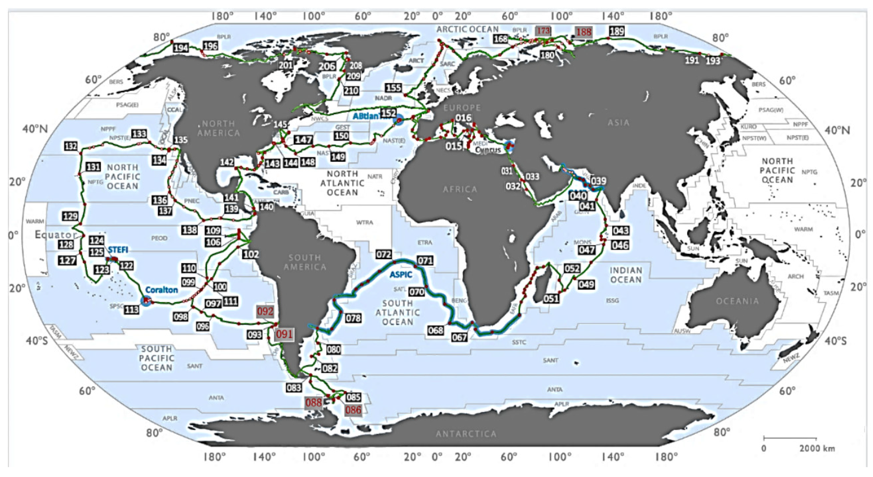
2.1. Data Sources

The TOP collected water samples from 210 sites were indicated by red dots in Figure 1, which was adopted and modified from Pesant et al. [3]. There were 102 sites with relatively complete data in the DCM layer. Three samples with abnormal value comparisons were shown in Figure 1. The raw data was obtained from http://ocean-microbiome.embl.de/data/OM.CompanionTables.xlsx (accessed on 1 October 2022).

2.2. Data Cleaning

The samples number was limited due to the difficulty of and financial investment required for ocean investigation. Samples contained detection errors and other inconsistencies, and some of them were partial or incomplete. Anomalous data may be caused by specific conditions such as location, bioturbation, and the influence of ocean currents. Extremely abnormal data was excluded, and data that were not suitable for modeling according to marine environmental indicators were also excluded from the further analysis.

For a sample matrix ${\mathrm{S}}_{\mathrm{m}\times \mathrm{n}}$,

$${\mathrm{S}}_{\mathrm{m}\times \mathrm{n}}=[\begin{array}{c}{\mathrm{S}}_0\\ ⋮\\ {\mathrm{S}}_{\mathrm{i}}\\ ⋮\\ {\mathrm{S}}_{\mathrm{m}-1}\end{array}]=[\begin{array}{ccc}{\mathrm{S}}_{00}& \cdots & {\mathrm{S}}_{0\left(\mathrm{n}-2\right)}\\ ⋮& \ddots & ⋮\\ {\mathrm{S}}_{\left(\mathrm{m}-1\right)0}& \cdots & {\mathrm{S}}_{\left(\mathrm{m}-1\right)\left(\mathrm{n}-2\right)}\end{array}\begin{array}{c}{\mathrm{S}}_{0\left(\mathrm{n}-1\right)}\\ ⋮\\ {\mathrm{S}}_{\left(\mathrm{m}-1\right)\left(\mathrm{n}-1\right)}\end{array}]$$

(1)

where vector ${\mathrm{S}}_{\mathrm{i}}$ represents sample data in the original samples and vector ${\mathrm{S}}_{\mathrm{ij}}$ represents the $\mathrm{jth}$ factor in the $\mathrm{ith}$ original sample.

The sample points evaluation vector was ${\mathrm{E}}_{\mathrm{n}}$,

$${\mathrm{E}}_{1\times \mathrm{m}}=[{\mathrm{E}}_0,\dots ,{\mathrm{E}}_{\mathrm{m}-1}]$$

(2)

where ${\mathrm{E}}_{\mathrm{i}}$ was the sample evaluation weight of the $\mathrm{ith}$ sample. The ${{\mathrm{E}}_{\mathrm{i}}}^{’}$s value was set according to the characteristics of the sample, such as the location, distance from other points and density of nearby sample points. ${\displaystyle \sum }{\mathrm{E}}_{\mathrm{i}}=1$, and ${\mathrm{E}}_{\mathrm{i}}\in [0,1]$.

We calculated the value of $\mathrm{E}\times \mathrm{S}$ to obtain the sample reference vector ${\mathrm{B}}_{\mathrm{n}}$,

$${\mathrm{B}}_{1\times \mathrm{n}}=\left(\mathrm{E}\times \mathrm{S}\right)/\mathrm{m}=[{\mathrm{B}}_0,\dots ,{\mathrm{B}}_{\mathrm{n}-1}]$$

(3)

and built the sample evaluation matrix ${\mathrm{V}}_{\mathrm{m}\times \mathrm{n}}$,

$${\mathrm{V}}_{\mathrm{m}\times \mathrm{n}}=[\begin{array}{ccc}{\mathrm{V}}_{00}& \cdots & {\mathrm{V}}_{0\left(\mathrm{n}-2\right)}\\ ⋮& \ddots & ⋮\\ {\mathrm{V}}_{\left(\mathrm{m}-1\right)0}& \cdots & {\mathrm{V}}_{\left(\mathrm{m}-1\right)\left(\mathrm{n}-2\right)}\end{array}\begin{array}{c}{\mathrm{V}}_{0\left(\mathrm{n}-1\right)}\\ ⋮\\ {\mathrm{V}}_{\left(\mathrm{m}-1\right)\left(\mathrm{n}-1\right)}\end{array}]$$

(4)

${\mathrm{V}}_{\mathrm{ij}}$ is obtained from Equations (3) and (4),

$${\mathrm{V}}_{\mathrm{ij}}=\{\begin{array}{l}1, {\mathrm{S}}_{\mathrm{ij}}\langle \mathsf{\alpha }\times {\mathrm{B}}_{\mathrm{j}} \mathrm{or} {\mathrm{S}}_{\mathrm{ij}}\rangle \mathsf{\beta }\times {\mathrm{B}}_{\mathrm{j}} \\ 0, \mathrm{else}\end{array}$$

(5)

where $\mathsf{\alpha }$ and $\mathsf{\beta }$ were the upper and lower limit coefficients of evaluation.

Next, we built the sample attribute selection matrix,

$${\mathsf{\delta }}_{\mathrm{m}\times 1}=[\begin{array}{c}{\mathsf{\delta }}_0\\ ⋮\\ {\mathsf{\delta }}_{\mathrm{i}}\\ ⋮\\ {\mathsf{\delta }}_{\mathrm{m}-1}\end{array}]$$

(6)

where ${\mathsf{\delta }}_{\mathrm{i}}=\{\begin{array}{l}0, \left({\mathsf{\eta }\mathrm{V}}_{\mathrm{i}\left(\mathrm{n}-1\right)}+{\displaystyle \sum }_{\mathrm{j}=0}^{\mathrm{n}-2}{\mathrm{V}}_{\mathrm{ij}}/\mathsf{\xi }\right)\ge 1\\ 1, \mathrm{else}\end{array}$.

The coefficients $\mathsf{\eta }$ and $\mathsf{\xi }$ were the target weight coefficient and the other attribute’s weight coefficient, respectively. For the single tag predictive value, $\mathsf{\eta }=1 \mathrm{and} \mathsf{\xi }\ge 1$.

Finally, the sample was cleaned according to the value of ${\mathsf{\delta }}_{\mathrm{i}}$ in the sample attribute selection matrix $\mathsf{\delta }$, where ${\mathsf{\delta }}_{\mathrm{i}}$ = 1 indicates that sample ${\mathrm{S}}_{\mathrm{i}}$ was reserved; otherwise, the sample was abandoned and was not used in subsequent modeling analysis.

3. Comprehensive Correlation Model

3.1. Character Importance

The RF algorithm was a decision tree-based packaged ensemble learning method that combines the advantages of boost-strap aggregation and random decision forests to improve the computing decision-making performance. It has good tolerance to noise and outliers. It also has good stability when dealing with large dimensional data problems. In this study, the Gini index was used to calculate the purity of the nodes and measure the characteristic importance index of marine environmental factors to Chl-a.

The Gini importance score ${\mathrm{VIM}}_{\mathrm{j}}$ was obtained according to the Gini index changes before and after the decision tree branches of the RF. The Gini index can be calculated by Equation (7).

$$\mathrm{Gini} \left(\mathrm{p}\right)={{\displaystyle \sum }}_{\mathrm{k}=1}^{\mathrm{K}}{\mathrm{p}}_{\mathrm{k}}\left(1-{\mathrm{p}}_{\mathrm{k}}\right)=1-{{\displaystyle \sum }}_{\mathrm{k}=1}^{\mathrm{K}}{\mathrm{p}}_{\mathrm{k}}^2,$$

(7)

where K represents the number of categories of feature samples, and $p_k$ represents the sample weight of the $\mathrm{kth}$ category in all nodes. The importance of feature ${\mathrm{X}}_{\mathrm{j}}$ at node $\mathrm{m}$ is the Gini index change before and after node $\mathrm{m}$ branches.

$${\mathrm{VIM}}_{\mathrm{jm}}^{\left(\mathrm{gini}\right)}={ \mathrm{GI}}_{\mathrm{m}}-{\mathrm{GI}}_{\mathrm{l}}-{\mathrm{GI}}_{\mathrm{r}},$$

(8)

where ${\mathrm{GI}}_{\mathrm{l}}$ and ${\mathrm{GI}}_{\mathrm{r}}$ represent the Gini index of two new nodes after node splitting. The importance of feature ${\mathrm{X}}_{\mathrm{j}}$ on the$\mathrm{i}$ tree was

$${\mathrm{VIM}}_{\mathrm{jm}}^{\left(\mathrm{gini}\right)}={{\displaystyle \sum }}_{\mathrm{m}\in \mathrm{M}}{\mathrm{VIM}}_{\mathrm{jm}}^{\left(\mathrm{gini}\right)}$$

(9)

If there were $\mathrm{n}$ trees in the RF, the importance of feature ${\mathrm{X}}_{\mathrm{j}}$ can be obtained by summing

$${ \mathrm{VIM}}_{\mathrm{j}}^{\left(\mathrm{gini}\right)}={{\displaystyle \sum }}_{\mathrm{m}=1}^{\mathrm{n}}{\mathrm{VIM}}_{\mathrm{jm}}^{\left(\mathrm{gini}\right)}$$

(10)

Finally, the final characteristic Gini index can be obtained by normalization of all the obtained importance factors:

$${\mathrm{VIM}}_{\mathrm{j}}=\frac{{\mathrm{VIM}}_{\mathrm{j}}}{{{\displaystyle \sum }}_{\mathrm{i}=1}^{\mathrm{c}}{\mathrm{VIM}}_{\mathrm{i}}}$$

(11)

3.2. Pearson Correlation

The Pearson correlation coefficient was used to measure the degree of correlation between two variables. It was defined as the quotient of covariance and standard deviation between two variables.

$${\mathsf{\rho }}_{\mathrm{x},\mathrm{y}}=\frac{\mathrm{cov}\left(\mathrm{X},\mathrm{Y}\right)}{{\mathsf{\sigma }}_{\mathrm{X}}{\mathsf{\sigma }}_{\mathrm{Y}}},$$

(12)

where $\mathrm{cov}\left(\mathrm{X},\mathrm{Y}\right)$ was the covariance of sample $\mathrm{X}$ and $\mathrm{Y}$, ${ \mathsf{\sigma }}_{\mathrm{X}}$ and ${\mathsf{\sigma }}_{\mathrm{y}}$ are the expected root values of variables $\mathrm{X}$ and $\mathrm{Y}$, ${\mathsf{\rho }}_{\mathrm{x},\mathrm{y}}$ was the degree of correlation between variables $\mathrm{X}$ and $\mathrm{Y}$, and the value range is $-1\le {\mathsf{\rho }}_{\mathrm{x},\mathrm{y}}\le 1$. When ${\mathsf{\rho }}_{\mathrm{x},\mathrm{y}}$ = −1, it means that the two variables are completely negatively correlated, and when ${\mathsf{\rho }}_{\mathrm{x},\mathrm{y}}$ = 1, it means that the two variables are completely positively correlated.

By estimating the covariance and standard deviation of the sample, the Pearson correlation coefficient $\mathrm{r}$ can be obtained.

$$\mathrm{r} =\frac{{{\displaystyle \sum }}_{\mathrm{i}=1}^{\mathrm{n}}\left({\mathrm{X}}_{\mathrm{i}}-\overline{\mathrm{X}}\right)\left({\mathrm{Y}}_{\mathrm{i}}-\overline{\mathrm{Y}}\right)}{\sqrt{{{\displaystyle \sum }}_{\mathrm{i}=1}^{\mathrm{n}}{\left({\mathrm{X}}_{\mathrm{i}}-\overline{\mathrm{X}}\right)}^2}\sqrt{{{\displaystyle \sum }}_{\mathrm{i}=1}^{\mathrm{n}}{\left({\mathrm{Y}}_{\mathrm{i}}-\overline{\mathrm{Y}}\right)}^2}}$$

(13)

where $\overline{\mathrm{X}}$ and $\overline{\mathrm{Y}}$ are the sample means.

3.3. Comprehensive Correlation Evaluation Model

There are complex implicit correlations among various marine environmental factors. To establish a comprehensive correlation evaluation model for the marine environment, we should consider not only the direct correlation between a single index and label elements, but also comprehensively consider the complex interactions between multiple index data and the implicit relationship of label elements. This study attempted to consider the comprehensive impact of feature importance and the Pearson correlation. We established a comprehensive correlation coefficient evaluation model between marine environmental factors and Chl-a, expecting to enhance the accuracy of Chl-a prediction. The established comprehensive correlation evaluation model was shown in Equation (14).

$${\mathrm{M}}_{\mathrm{evaluate}}={\mathsf{\zeta }}_1\times {\mathrm{VIM}}_{\mathrm{j}}+{\mathsf{\zeta }}_2\times \mathsf{\rho }\left(\mathrm{x},\mathrm{y}\right),$$

(14)

where ${\mathsf{\zeta }}_1$ and ${ \mathsf{\zeta }}_2$ were the weight coefficients of feature importance and the Pearson correlation. The values were assigned according to the specific circumstances of the environmental factors and label factors.

4. Integrated Prediction Model

The relationships between Chl-a and the environmental factors were strongly nonlinear and the number of samples was not sufficient, which make it difficult to predict the Chl-a. Thus, the marine environment factors prediction model need to integrate XGBoost regression, LOOCV validation, MRE optimization and other strategies to achieve a better performance.

4.1. Extreme Gradient Boosting Regression

XGBoost is a scalable end-to-end tree boosting system that is widely used by data scientists to achieve state-of-the-art results in addressing many machine learning challenges (Chen, et al., 2016). In this study, XGBoost was employed for regression modeling.

The XGBoost algorithm can be expressed in a form of addition as shown in Equation (15).

$${\hat{\mathrm{y}}}_{\mathrm{i}}={{\displaystyle \sum }}_{\mathrm{k}=1}^{\mathrm{K}}{\mathrm{f}}_{\mathrm{k}}\left({\mathrm{x}}_{\mathrm{i}}\right),{ \mathrm{f}}_{\mathrm{k}}\in \mathrm{F},$$

(15)

where ${\hat{\mathrm{y}}}_{\mathrm{i}}$ represents the predicted value of the model, K represents the number of decision numbers, $\mathrm{F}$ corresponds to the set of all K regression trees, and $\mathrm{f}\left(\mathrm{x}\right)$ was one of the trees.

The goal of the XGBoost algorithm was to make the predicted value ${\hat{\mathrm{y}}}_{\mathrm{i}}$ of the tree group close to the real value ${\mathrm{y}}_{\mathrm{i}}$, and ensure that the method has maximum generalization ability. In the process of XGBoost learning, the ${ \mathrm{f}}_{\mathrm{k}}$ function was added to optimize the objective function and reduce the error between the predicted results and the actual values. Its objective function was defined as

$$\begin{array}{cc}{\mathrm{Ob}}_{\mathrm{j}}& =\end{array}{{\displaystyle \sum }}_{\mathrm{i}=1}^{\mathrm{n}}\mathrm{l}\left({\mathrm{y}}_{\mathrm{i}},{\hat{\mathrm{y}}}_{\mathrm{i}}\right)+{{\displaystyle \sum }}_{\mathrm{i}=1}^{\mathrm{t}}\mathsf{\Omega } \left({\mathrm{f}}_{\mathrm{i}}\right),$$

(16)

The loss function ${{\displaystyle \sum }}_{\mathrm{i}=1}^{\mathrm{n}}\mathrm{l}\left({\mathrm{y}}_{\mathrm{i}},{\hat{\mathrm{y}}}_{\mathrm{i}}\right)$ refers to the error between the actual value and the predicted result from the XGBoost, and it’s the sum of the error of each iteration in the XGBoost modeling.

$$\mathsf{\Omega } \left({\mathrm{f}}_{\mathrm{i}}\right)\mathsf{\gamma }\mathrm{T}+\frac{1}{2}\mathsf{\lambda }{\left|\left|\mathsf{\omega }\right|\right|}^2,$$

(17)

where $\mathrm{T}$ represents the number of leaf nodes, $\mathsf{\omega }$ represents the fraction of leaf nodes, and γ and λ represent regularization coefficients to prevent the decision tree from being too complicated.

$$\mathrm{f}\left(\mathrm{x}+{\mathsf{\Delta }}_{\mathrm{x}}\right)\cong \mathrm{f}\left(\mathrm{x}\right)+{\mathrm{f}}_{\left(\mathrm{x}\right)}^{\prime }\mathsf{\Delta }\mathrm{x}+\frac{1}{2} {\mathrm{f}}^{″}\left(\mathrm{x}\right){\mathsf{\Delta }\mathrm{x}}^2$$

(18)

$${\mathrm{Obj}}_{\mathrm{j}}^{\left(\mathrm{t}\right)}\cong {{\displaystyle \sum }}_{\mathrm{i}=1}^{\mathrm{n}}\mathrm{l}[{\mathrm{y}}_{\mathrm{i}},{\hat{\mathrm{y}}}_{\mathrm{i}}^{\left(\mathrm{t}-1\right)}]+\mathsf{\Omega }\left({\mathrm{f}}_{\mathrm{t}}\right)+\mathsf{\epsilon }$$

(19)

In Equation (19), $\mathrm{l}\left({\mathrm{y}}_{\mathrm{i}},{\hat{\mathrm{y}}}_{\mathrm{i}}{}^{\left(\mathrm{t}-1\right)}\right)$ is the error function, $\mathsf{\Omega }\left({\mathrm{f}}_{\mathrm{t}}\right)$ was the regular term, and $\mathsf{\epsilon }$ was a constant for the complexity of the first T-1 tree.

Taylor-class expansion is carried out for the objective function, which was to combine Equation (18) with Equation (19),

$${\mathrm{Obj}}_{\mathrm{j}}^{\left(\mathrm{t}\right)}\cong {{\displaystyle \sum }}_{\mathrm{i}=1}^{\mathrm{n}}[\mathrm{l}({\mathrm{y}}_{\mathrm{i}},{\hat{\mathrm{y}}}_{\mathrm{i}}{}^{\left(\mathrm{t}-1\right)})+{\mathrm{g}}_{\mathrm{i}}{\mathrm{f}}_{\mathrm{t}}\left({\mathrm{x}}_{\mathrm{i}}\right)+\frac{1}{2}{\mathrm{h}}_{\mathrm{i}}{\mathrm{f}}_{\mathrm{t}}^2\left({\mathrm{x}}_{\mathrm{i}}\right)]+\mathsf{\Omega }\left({\mathrm{f}}_{\mathrm{t}}\right)+\mathsf{\epsilon },$$

(20)

where

$${ \mathrm{g}}_{\mathrm{i}}=\frac{\partial \mathrm{l}\left({\mathrm{y}}_{\mathrm{i}},{\hat{\mathrm{y}}}_{\mathrm{i}}{}^{\left(\mathrm{t}-1\right)}\right)}{\partial {\hat{\mathrm{y}}}_{\mathrm{i}}{}^{\left(\mathrm{t}-1\right)}},{ \mathrm{h}}_{\mathrm{i}}=\frac{{\partial }^2\mathrm{l}\left({\mathrm{y}}_{\mathrm{i}},{\hat{\mathrm{y}}}_{\mathrm{i}}{}^{\left(\mathrm{t}-1\right)}\right)}{{\partial }^2{\hat{\mathrm{y}}}_{\mathrm{i}}{}^{\left(\mathrm{t}-1\right)}}$$

(21)

In combination with Equations (19)–(21), the deformation was as follows:

$$\begin{gathered} {\mathrm{Obj}}_{\mathrm{j}}^{\left(\mathrm{t}\right)}\cong {{\displaystyle \sum }}_{\mathrm{i}=1}^{\mathrm{n}}[{\mathrm{g}}_{\mathrm{i}}{\mathrm{f}}_{\mathrm{t}}\left({\mathrm{x}}_{\mathrm{i}}\right)+\frac{1}{2}{\mathrm{h}}_{\mathrm{i}}{\mathrm{f}}_{\mathrm{t}}^2\left({\mathrm{x}}_{\mathrm{i}}\right)]+\mathsf{\Omega } \left({\mathrm{f}}_{\mathrm{t}}\right), \\ ={{\displaystyle \sum }}_{\mathrm{i}=1}^{\mathrm{n}}[{\mathrm{g}}_{\mathrm{i}}{\mathrm{f}}_{\mathrm{t}}\left({\mathrm{x}}_{\mathrm{i}}\right)+\frac{1}{2}{\mathrm{h}}_{\mathrm{i}}{\mathrm{f}}_{\mathrm{t}}^2\left({\mathrm{x}}_{\mathrm{i}}\right)]+\mathsf{\gamma }\mathrm{T}+\mathsf{\lambda }\frac{1}{2}{{\displaystyle \sum }}_{\mathrm{j}=1}^{\mathrm{T}}{\mathsf{\omega }}_{\mathrm{j}}^2, \\ ={{\displaystyle \sum }}_{\mathrm{j}=1}^{\mathrm{T}}[({{\displaystyle \sum }}_{\mathrm{i}\in {\mathrm{I}}_{\mathrm{j}}}{\mathrm{g}}_{\mathrm{i}}){\mathsf{\omega }}_{\mathrm{j}}+\frac{1}{2}({{\displaystyle \sum }}_{\mathrm{i}\in {\mathrm{I}}_{\mathrm{j}}}{\mathrm{h}}_{\mathrm{i}}+ \mathsf{\lambda }){\mathsf{\omega }}_{\mathrm{j}}^2]+ \mathsf{\gamma }\mathrm{T} \end{gathered}$$

(22)

${\mathrm{I}}_{\mathrm{j}}$ was defined for each leaf node j collection of the above samples in the table below, ${\mathrm{I}}_{\mathrm{j}}=${$\mathrm{i}$|$\mathrm{q}$(${\mathrm{x}}_{\mathrm{i}}$)=$\mathrm{j}$}, ${\mathrm{g}}_{\mathrm{i}}$ was the first derivative, and ${\mathrm{h}}_{\mathrm{i}}$ is the second derivative. Define ${\mathrm{G}}_{\mathrm{j}}$=${\displaystyle \sum }_{\mathrm{i}\in {\mathrm{I}}_{\mathrm{j}}}{\mathrm{g}}_{\mathrm{i}}$, ${\mathrm{H}}_{\mathrm{j}}=$ ${\displaystyle \sum }_{\mathrm{i}\in {\mathrm{I}}_{\mathrm{j}}}{\mathrm{h}}_{\mathrm{i}}$, and Equation (22) can be simplified as

$$\begin{gathered} {\mathrm{Obj}}_{\mathrm{j}}^{\left(\mathrm{t}\right)}={{\displaystyle \sum }}_{\mathrm{j}=1}^{\mathrm{T}}[\left({{\displaystyle \sum }}_{\mathrm{i}\in {\mathrm{I}}_{\mathrm{j}}}{\mathrm{g}}_{\mathrm{i}}\right){\mathsf{\omega }}_{\mathrm{j}}+\frac{1}{2}\left({{\displaystyle \sum }}_{\mathrm{i}\in {\mathrm{I}}_{\mathrm{j}}}{\mathrm{h}}_{\mathrm{i}}+ \mathsf{\lambda }\right){\mathsf{\omega }}_{\mathrm{j}}^2]+ \mathsf{\gamma }\mathrm{T}, \\ ={{\displaystyle \sum }}_{\mathrm{j}=1}^{\mathrm{T}}[{\mathrm{G}}_{\mathrm{j}}{\mathsf{\omega }}_{\mathrm{j}}+\frac{1}{2}\left({\mathrm{H}}_{\mathrm{j}}+ \mathsf{\lambda }\right){\mathsf{\omega }}_{\mathrm{j}}^2]+ \mathsf{\gamma }\mathrm{T}. \end{gathered}$$

(23)

Equation (23) showed that the objective function ${\mathrm{Obj}}_{\mathrm{j}}^{\left(\mathrm{t}\right)}$ was a convex function. The optimal solution of the objective function can be obtained by taking the derivative of ${\mathsf{\omega }}_{\mathrm{j}}$.

$${\mathsf{\omega }}_{\mathrm{j}}^{\ast }=-\mathrm{GjHj}+ \mathsf{\lambda }$$

(24)

$${\mathrm{Obj}}_{\mathrm{j}}^{\left(\mathrm{t}\right)}=-\frac{1}{2}{{\displaystyle \sum }}_{\mathrm{j}=1}^{\mathrm{T}}\frac{{\mathrm{G}}_{\mathrm{j}}{}^2}{{\mathrm{H}}_{\mathrm{j}}+\mathsf{\lambda }}+ \mathsf{\gamma }\mathrm{T}$$

(25)

According to the results of ${\mathsf{\omega }}_{\mathrm{j}}^{\ast }$ and ${\mathrm{Obj}}_{\mathrm{j}}^{\left(\mathrm{t}\right)}$, Equation (17) can evaluate the quality of the tree model. The smaller the value of ${\mathrm{Obj}}_{\mathrm{j}}^{\left(\mathrm{t}\right)}$, the better the tree model. The scoring formula for splitting can be obtained as follows:

$$\mathrm{Gain} =\frac{1}{2}[\frac{{({{\displaystyle \sum }}_{\mathrm{i}\in {\mathrm{I}}_{\mathrm{L}}}{\mathrm{g}}_{\mathrm{i}})}^2}{{{\displaystyle \sum }}_{\mathrm{i}\in {\mathrm{I}}_{\mathrm{L}}}{\mathrm{h}}_{\mathrm{i}}+\mathsf{\lambda }}+\frac{{({{\displaystyle \sum }}_{\mathrm{i}\in {\mathrm{I}}_{\mathrm{R}}}{\mathrm{g}}_{\mathrm{i}})}^2}{{{\displaystyle \sum }}_{\mathrm{i}\in {\mathrm{I}}_{\mathrm{R}}}{\mathrm{h}}_{\mathrm{i}}+\mathsf{\lambda }}+\frac{{\left({{\displaystyle \sum }}_{\mathrm{i}\in \mathrm{I}}{\mathrm{g}}_{\mathrm{i}}\right)}^2}{{{\displaystyle \sum }}_{\mathrm{i}\in \mathrm{I}}{\mathrm{g}}_{\mathrm{i}}+\mathsf{\lambda }}]-\mathsf{\gamma }.$$

(26)

Equation (26) was used to calculate the split nodes of the tree model, where ${\mathrm{I}}_{\mathrm{L}}$ and ${\mathrm{I}}_{\mathrm{R}}$ were the real sets of the split left node and right node and $\mathrm{I}$ was the whole instance set.

4.2. LOOCV Validation

Due to the limited number of valid samples in this study, it was critical to select an appropriate validation method to ensure the accuracy and generalization ability of the Chl-a prediction in the multi-environmental factor prediction model. LOOCV was a special case of cross-validation in which the number of folds was equal to the number of instances in the dataset. Thus, the learning algorithm was applied once for each sample, using all other samples as a training set and using the selected sample as a single-item test set (Webb et al. 2011). LOOCV was adopted for the validation of Chl-a in the multi-environmental factors prediction model. The smaller sample size avoids the disadvantages of the computational complexity of the LOOCV method in dealing with large samples, but it didn’t affect the model’s prediction accuracy.

4.3. Objective for Prediction

To ensure the subsequent modeling training and prediction validation values of Chl-a, mean relative error (MRE) was defined as

$$\mathrm{MRE}=\frac{1}{\mathrm{M}}{\displaystyle \sum }_{\mathrm{t}=1}^{\mathrm{M}}\frac{\left|{\mathrm{z}}_{\mathrm{i}}-{\hat{\mathrm{z}}}_{\mathrm{i}}\right|}{\left|{\mathrm{z}}_{\mathrm{i}}\right|}$$

(27)

where ${\mathrm{z}}_{\mathrm{i}}$ was the real value of the sample labels of Chl-a, and ${\hat{\mathrm{z}}}_{\mathrm{i}}$ is the predicted value of the Chl-a. The objection function for the Chl-a prediction model was to obtain the minimum MRE:

$$\mathrm{Min}\left(\frac{1}{\mathrm{M}}{{\displaystyle \sum }}_{\mathrm{t}=1}^{\mathrm{M}}\frac{\left|{\mathrm{z}}_{\mathrm{i}}-{\hat{\mathrm{z}}}_{\mathrm{i}}\right|}{\left|{\mathrm{z}}_{\mathrm{i}}\right|}\right)$$

(28)

5. Results and Discussion

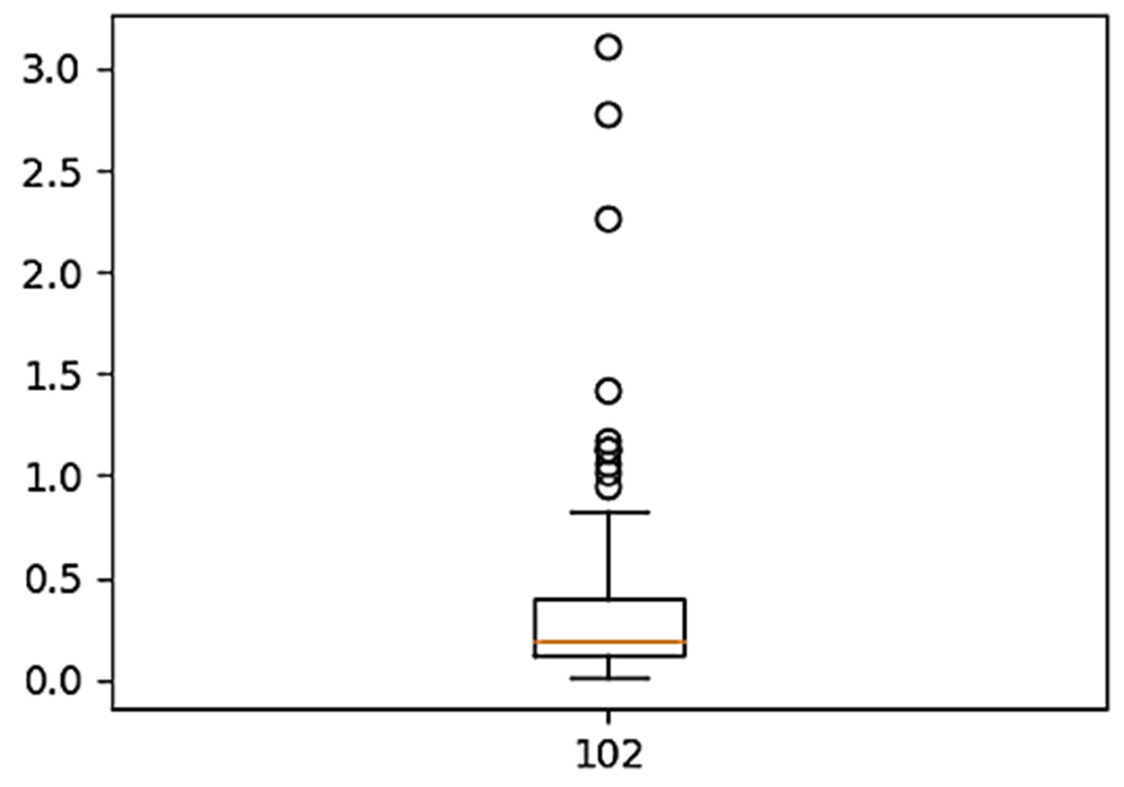
5.1. Raw Data Processing

Figure 2 showed the distribution of Chl-a content in 102 original samples in the form of a box plot in order to illustrate the existence of outliers in the original samples. The abscissa was the sample size, and the ordinate was the content of Chl-a in those samples. It can be seenthat some Chl-a values were abnormally large or small.

There were 15 environmental factors that can be used for modeling and prediction including temperature (Temp), oxygen (Oxy), density (Den), carbonate (CO₃), ammonium (Amm), Brunt Väisälä frequency (Bru), salinity (Sal), ${\mathrm{PO}}_4$ iron (Iron), latitude (Lat), ${\mathrm{NO}}_2$ gradient surface temperature (Gra), beta470(Beta), Okubo (Oku), and longitude (Long). The target object was set to the Chl-a. Several samples had outlier Chl-a values, and the samples adjacent to them were presented in

Table 1. Samples with outlier Chl-a values and samples adjacent to them.

Station	Chl-a	Long	Lat	Temp	Den	Oxygen	CO3	Amm
TARA_091	0.828	−73.100	−34.161	17.609	24.893	229.394	0.013	0.048
TARA_092	2.258	−71.998	−33.690	15.912	25.302	245.324	0.013	0.073
TARA_086	0.220	−53.006	−64.360	−0.494	26.718	398.312	0.000	0.007
TARA_088	1.129	−56.794	−63.402	−0.763	27.684	335.243	0.013	0.118
TARA_173	0.417	79.420	78.956	−0.160	26.994	385.281	0.001	0.004
TARA_188	1.417	91.856	78.252	−1.650	26.511	388.304	0.000	0.002

. Some environmental indicators in one sample might be quite different from a nearby sample, even if they were in the same area. The wide-ranging differences in Chl-a might be caused by some accidental event or systematic error, or other potential causes that have not yet been discovered. Such a distribution pattern might be caused by unknown topography, ocean currents, seasonal changes, human activity and other factors. A detailed and accurate description of the distribution of global marine environmental indicators cannot be developed based on the samples acquired to date. Accurate interpretation and in-depth study of these abnormal indicators require more comprehensive samples, targeted field tests, in-depth theoretical analysis, and artificial intelligence learning. Based on the data cleaning model used in this study, total 79 samples from the SRF layer were selected and subjected to the consequential analysis.

5.2. Evaluation of Characteristic Importance of Environmental Factors

Based on these selected data, the modeling analysis and the prediction were then conducted with regard to the relationship between Chl-a and other environmental factors in the SRF layer. The characteristic importance of each marine environmental factor to Chl-a was obtained through characteristic importance data analysis technology. The distribution of the characteristic importance indexes of each environmental factor was presented in Figure 3. The major parameters for the evaluation were listed in

Table 2. Five parameters used for the calculation of the characteristic importance.

Parameters	N_Estimators	Min_Samples _Split	Min_Samples _Leaf	Min_Weight _Fraction_Leaf	Max_Depth
Values	100	2	1	0	2

, where n_estimators was the number of trees in the forest, min_samples_split was the minimum number of samples required to split an internal node, min_samples_leaf is the minimum number of samples required to be at a leaf node, min_weight_fraction_leaf is the minimum weighted fraction of the sum total of weights required to be at a leaf node, and max_depth is the maximum depth of the tree. As shown in Figure 3, the characteristic importance analysis indicate that seawater density was the most important factor in terms of Chl-a abundance for the samples from the SRF layer. Seven factors including temperature, latitude, bate470, oxygen, ammonium, CO₃, and Brunt Väisälä frequency were also important in regard to Chl-a abundance. However, seven factors including the Okubo, PO₄, salinity, NO₂, gradient surface temperature, iron and longitude on the abundance of Chl-a demostrated no obvious importance.

The Pearson correlation method was used to further study the effects of environmental factors on the Chl-a abundance. Figure 4 presented the Pearson correlation coefficient of each marine environment factor and Chl-a. As shown in Figure 4, the strongest positive correlation between the oxygen content and Chl-a was observed. The strongest negative correlation between water temperature and Chl-a was also found. The correlation coefficients of CO₃, density, and PO₄ were 0.397, 0.339 and 0.226, respectively. The relative values of the Brunt Väisälä frequency and salinity were −0.270 and −0.264. However, the correlation between other factors and Chl-a was not obvious.

By comparing Figure 3 and Figure 4, it can be seen that Pearson’s correlation coefficient, which not only indicated the direct correlation between the two environmental indicators, but also provided the characteristic importance index, cannot fully reflect impact on the abundance of Chl-a. Given the potential correlation of multiple environmental factors in the global ocean and the limited number of samples available, Equation (14) was used to calculate the Chl-a comprehensive correlation index. In this study, the weight coefficients ${\mathsf{\zeta }}_1$ and ${\mathsf{\zeta }}_2$ of feature importance and Pearson correlation were set as 0.5 and 0.5.

Since the characteristic importance of the environmental factors was normalized, the Pearson correlation coefficients were also normalized. The Pearson correlation coefficient, characteristic importance index, and comprehensive correlation index are presented in

Table 3. Comprehensive correlation indexes.

Parameter	Character Importance Index	Pearson Correlation Coefficient	Normalized Pearson Correlation Coefficient	Comprehensive Correlation Index
Density	0.151	0.339	0.091	0.129
Temperature	0.103	−0.575	0.154	0.121
Latitude	0.098	0.106	0.028	0.121
Beta470	0.089	0.050	0.013	0.089
Oxygen	0.080	0.600	0.161	0.079
Ammonium	0.080	0.290	0.078	0.070
CO3	0.070	0.397	0.107	0.063
Bru	0.067	−0.270	0.073	0.055
Okubo	0.054	0.068	0.018	0.051
PO4	0.041	0.226	0.061	0.051
Salinity	0.040	−0.264	0.071	0.040
NO2	0.037	0.158	0.042	0.039
Gra	0.037	0.120	0.032	0.036
Iron	0.027	−0.187	0.050	0.035
Longitude	0.027	0.072	0.019	0.023

. The histogram of the comprehensive correlation indexes was drawn in Figure 5. As shown in Figure 5 and Table 3, four environmental factors including the temperature, density, oxygen and CO₃ have the greatest influence on the abundance of Chl-a, while the comprehensive correlation indexes of the other factors were relative low.

5.3. Environmental Factors Modeling

The environmental characteristic importance model can be used to identify easily-detected and easily-measured factors that can be used to predict other factors that were not directly measured in previous explorations. Thus, rapid and low-cost data acquisition in marine development, exploration, and environmental protection may be possible. This study used XGBoost, RF, SVR and LR to implement multi-factor modeling, analysis, and prediction.

As shown in Figure 5, density, temperature, oxygen, and CO₃ had the highest comprehensive correlation values. In the modeling prediction study, the modeling began with the four most important indicators. Then, a new environmental factor was added successively according to the comprehensive correlation indexes from high to low, until all the factors were used. The modeling and prediction process was constructed based on several algorithms, including the XGBoost algorithm. The objective function was to minimize the MRE with Equation (28).

Table 4. Four environmental factors used for modeling analysis.

	XGBoost	RF	SVR	Linear Regression
MRE	0.398	0.413	0.461	0.532
MAE	0.096	0.104	0.110	0.118
RMSE	0.144	0.152	0.155	0.166
R2	0.550	0.496	0.470	0.390

,

Table 5. Five environmental factors used for modeling.

	XGBoost	RF	SVR	Linear Regression
MRE	0.408	0.421	0.459	0.549
MAE	0.096	0.103	0.109	0.114
RMSE	0.142	0.148	0.154	0.157
R2	0.56	0.522	0.488	0.462

,

Table 6. Six environmental factors used for modeling.

	XGBoost	RF	SVR	Linear Regression
MRE	0.419	0.425	0.446	0.572
MAE	0.107	0.104	0.112	0.12
RMSE	0.152	0.151	0.155	0.160
R2	0.501	0.508	0.470	0.430

and

Table 7. Eight environmental factors used for modeling.

	XGBoost	RF	SVR	Linear Regression
MRE	0.344	0.378	0.447	0.562
MAE	0.083	0.086	0.112	0.125
RMSE	0.125	0.127	0.158	0.169
R2	0.660	0.649	0.460	0.370

showed the MRE, mean absolute error (MAE), root mean square error (RMSE), and the sum of squares of the residuals R² with different machine learning algorithms. As can be seen that no matter whether the number of environmental factors is four, five, six, or eight, the MRE obtained based on XGBoost regression is superior to that of the other methods. The results presented in Table 5 and Table 7 show that whether the model is based on five, six or eight environmental factors, the MRE, RMSE, and R² of based on XGBoost algorithm are better than those obtained with the other centralized machine learning algorithms. In Table 4 and Table 6, the MRE and RMSE based on XGBoost were slightly higher than those of RF, and less than those of SVR and LR. Because of the large difference in the Chl-a values in the raw samples, the MRE results show that the prediction results based on the XGBoost model were more reasonable.

5.4. Chl-a Abundance Prediction

Predictions were developed and the objective function model was established using Equation (28). Figure 6 showed the relative errors of each prediction. The modeling and prediction results obtained with the XGBoost algorithm were sorted from small to large in Figure 6. In general, the more environmental factors used for modeling, the smaller the relative error of the prediction of the trained model. In the prediction of Chl-a abundance, the number of sample points with a large relative error was greater with the LR algorithm than with the SVR or RF algorithms, and was least with the XGBoost algorithm. Too few modeling parameters (e.g., four or five) led to many high MRE values, which indicates that modeling with too few parameters does not result in reliable Chl-a predictions. When the number of modeling parameters is six to eight, the number of outlier relative error values was close to the prediction results using more parameters. This indicates that it is feasible to use appropriate quantity parameters modeling to predict Chl-a. The effect of modeling with more parameters (e.g., 13 to 15) did not reduce the relative errors, but lead to an increase of outlier values instead.

It can be seen from Figure 6, the XGBoost, RF, SVR, and LR methods can be used for modeling and predicting the value of Chl-a. When RF and SVR were used for modeling and prediction, more large relative errors appeared in the results.

For further analysis of the modeling prediction results, the prediction tolerance ${\mathrm{M}}_{\mathrm{s}}$ was introduced. It represents the mean value of the$\mathrm{s}\%$ smallest average relative error of samples. ${\mathrm{M}}_{100}$ is the mean relative error of all samples and ${\mathrm{M}}_{60}$ is the mean relative error of the $60\%$ smallest relative error of samples. Figure 7 presents the s% smallest of the average relative error of samples by different machine learning methods. By comparing subgraphs (a)–(d) in Figure 7, it can be seen that for all the M_s, the modeling prediction results based on XGBoost were generally superior to the RF model. This method, and shows obvious advantages over SVR and LR. For the XGBoost and RF modeling methods, at first, the prediction accuracy of the target values improves gradually with the increase in the number of indices used for modeling. It is important to note that when the number of environmental factors is greater than five, the increase in prediction accuracy for XGBoost and RF is not obvious. For the SVR and LR methods, the prediction accuracy decreases with the increase of attributes of environmental factors initially. When the modeling factors were greater than eight, the increase in environmental factors has no obvious effect on the accuracy of prediction results.

Figure 7 presents the MRE of samples using different machine learning methods. It can be seen that the modeling prediction results based on XGBoost and RF were superior to those of SVR and LR.

A learning curve and grid search techniques were used in the model training to minimize the objective function (Equation (28)). The XGBoost regression analysis modeling process depends on several key parameters such as maximum tree depth (max_depth), number of trees (n_estimators), regularization term of the weight (reg_alpha), minimum loss function drop value (gamma), learning rate, subsample size (subsample), minimum node weight (min_child weight), and the proportion of the sampled columns (colsample_bytree). The optimization parameters of the training model were obtained by parameter estimation and cross-validation.

Table 8. Parameters of XGBoost.

Factor Numbers	Max Depth	N_Estimators	Reg_Alpha	Gamma	Learning Rate	Sub-Sample	Min_Child Weight	Colsample _Bytree
4	1	70	0	0	1	0.8	1	1
5	1	70	0	0	1	0.8	1	1
6	3	70	0.01	0	0.1	0.75	4	0.8
7	3	70	0.01	0	0.1	0.75	6	0.8
8	4	70	0.01	0	0.1	−0.75	7	0.8
9	3	70	0.001	0.1	0.1	0.8	5	0.8
10	3	70	0.1	0	0.1	0.75	7	0.8
11	3	70	0.1	0	0.1	0.85	5	0.75
12	3	70	0.001	0	0.1	0.85	7	0.85
13	3	70	0.1	0	0.1	0.8	3	0.75
14	3	70	0.01	0	0.1	0.85	3	0.75
15	3	70	0.1	0	0.1	0.85	3	0.8

presents the combination of the optimization parameters obtained using grid search technology for modeling a different number of environmental factors.

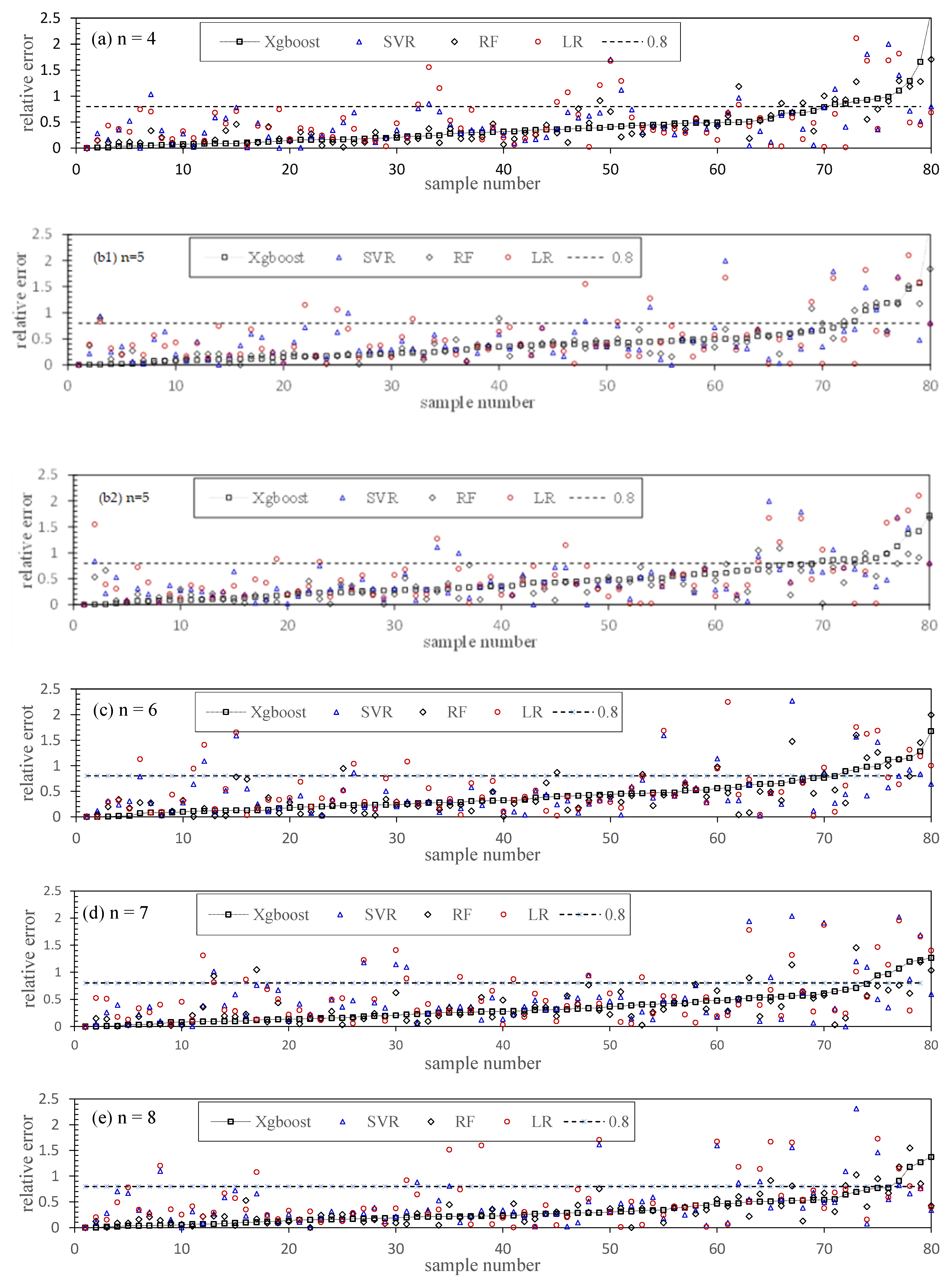
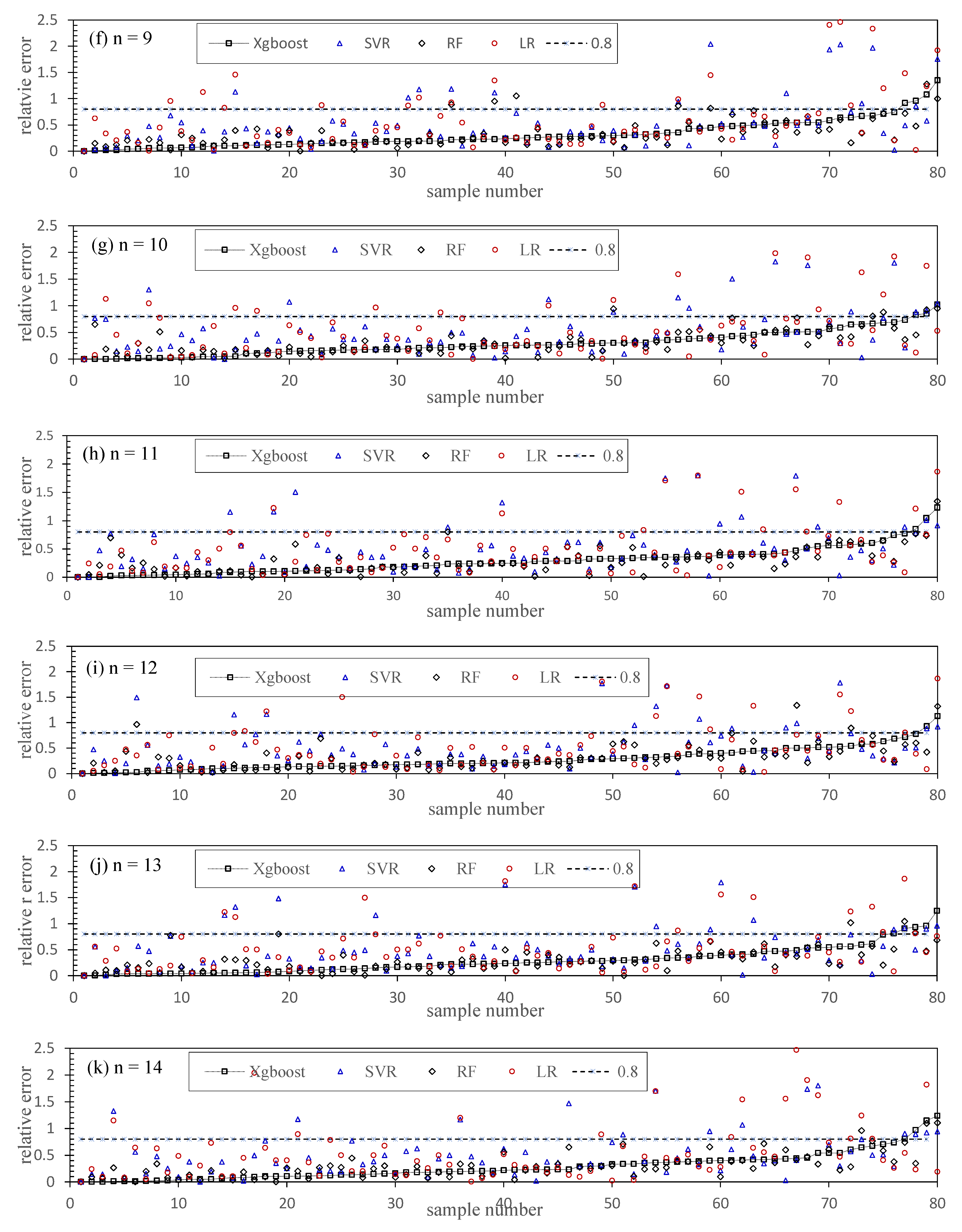
5.5. Modeling Optimization and Comparison

A grid search method was used for the parameter optimization of Max_depth and n_estimators, and the obtained results were shown in Figure 8. And the variation in the MRE according to the n_estimator values increasing under different Max_depth values were also included. It can be seen that, when the n_estimator exceeds 70, the MRE achieved a stable value in any case. The results of the MRE based on four, five, and six factors were very similar, and were higher than the results based on more factors. In general, more factors were included for modeling and prediction analysis, the higher rate of the accuracy of the analysis were obtained.

6. Conclusions

It’s of great importance to integrate and analyze elements of the marine environment, integrate multi-source, heterogeneous, and dispersed marine environment data, and reveal complex internal mechanisms and evolution trends through the machine learning method. Based on selected Tara Oceans data, the present study conducted in-depth data cleaning, multi-factor comprehensive correlation, and Chl-a abundance modeling and prediction. A marine environmental factors comprehensive correlation model and Chl-a abundance prediction model were then established based on the proposed machine learning analysis.

The conclusions of this study are as follows:

(1)

The comprehensive correlation model of marine environmental factors considers both the direct correlation between any two environmental factors and the potential correlation among multiple factors. It is helpful for the selection of factors for Chl-a modeling and prediction.

(2)

A multi-environmental factor prediction model can accurately predict the amount of Chl-a, which can help to determine Chl-a abundance on other indicators of the marine environment.

(3)

The more environmental factors used for Chl-a predicting, the more accurate the results will be. With increasing amounts of marine environmental data included, the machine learning technologies will be used for additional relevant studies. Revealing small-scale, refined and systematic laws of the marine environment requires additional marine observation, monitoring and measurement data. This approach will help to develop a deeper understanding of the underlying mechanisms behind the dynamic changes in the marine environment, and thus develop more efficient ways to protect the marine environment.

References

1. Madin, E.M.; Dill, L.M.; Ridlon, A.D.; Heithaus, M.R.; Warner, R.R. Human activities change marine ecosystems by altering predation risk. Glob. Chang. Biol. 2016, 22, 44–60. [Google Scholar] [CrossRef]
2. Biard, T.; Bigeard, E.; Audic, S.; Poulain, J.; Gutierrez-Rodriguez, A.; Pesant, S.; Stemmann, L.; Not, F. Biogeography and diversity of Collodaria (Radiolaria) in the global ocean. ISME J. 2017, 11, 1331–1344. [Google Scholar] [CrossRef] [PubMed] [Green Version]
3. Pesant, S.; Tara Oceans Consortium Coordinators; Not, F.; Picheral, M.; Kandels-Lewis, S.; Le Bescot, N.; Gorsky, G.; Iudicone, D.; Karsenti, E.; Speich, S.; et al. Open science resources for the discovery and analysis of Tara Oceans data. Sci. Data 2015, 2, 150023. [Google Scholar] [CrossRef] [Green Version]
4. Sunagawa, S.; Coelho, L.P.; Chaffron, S.; Kultima, J.R.; Labadie, K.; Salazar, G.; Djahanschiri, B.; Zeller, G.; Mende, D.R.; Alberti, A.; et al. Structure and function of the global ocean microbiome. Science 2015, 348, 6237. [Google Scholar] [CrossRef] [Green Version]
5. Karlusich, J.; Ibarbalz, F.M.; Bowler, C. Phytoplankton in the Tara Ocean. Annu. Rev. Mar. Sci. 2020, 12, 233–265. [Google Scholar] [CrossRef] [Green Version]
6. Zhang, X.L.; Yang, X.; Wang, S.J.; Jiang, Z.W.; Xie, Z.X.; Zhang, L. Draft Genome Sequences of Nine Cultivable Heterotrophic Proteobacteria Isolated from Phycosphere Microbiota of Toxic Alexandrium catenella LZT09. Microbiol. Resour. Announc. 2020, 9, e00281-20. [Google Scholar] [CrossRef]
7. Zhang, X.L.; Tian, X.Q.; Ma, L.Y.; Feng, B.; Liu, Q.H.; Yuan, L.D. Biodiversity of the symbiotic bacteria associated with toxic marine dinoflagellate Alexandrium tamarense. J. Biosci. Med. 2015, 3, 23–28. [Google Scholar] [CrossRef] [Green Version]
8. Zhang, X.L.; Ma, L.Y.; Tian, X.Q.; Huang, H.L.; Yang, Q. Biodiversity study of intracellular bacteria closely associated with paralytic shellfish poisoning dinoflagellates Alexandrium tamarense and A. minutum. Int. J. Environ. Resour. 2015, 4, 23–27. [Google Scholar] [CrossRef]
9. Xu, G.; Shi, Y.; Sun, X.; Shen, W. Internet of Things in Marine Environment Monitoring: A Review. Sensors 2019, 19, 1711. [Google Scholar] [CrossRef] [Green Version]
10. Bonnefon, J.F.; Rahwan, I. Machine Thinking, Fast and Slow. Trends Cogn. Sci. 2020, 24, 1019–1027. [Google Scholar] [CrossRef] [PubMed]
11. Sunagawa, S.; Karsenti, E.; Bowler, C.; Bork, P. Computational eco-systems biology in Tara Oceans: Translating data into knowledge. Mol. Syst. Biol. 2015, 11, 809. [Google Scholar] [CrossRef] [PubMed]
12. Bork, P.; Bowler, C.; Vargas, C.D.; Gorsky, G. Tara oceans-studies plankton at planetary scale. Science 2015, 384, 873. [Google Scholar] [CrossRef] [PubMed] [Green Version]
13. Yang, Q.; Jiang, Z.; Zhou, X.; Zhang, R.; Xie, Z.; Zhang, S.; Wu, Y.; Ge, Y.; Zhang, X. Haliea alexandrii sp. nov., isolated from phycosphere microbiota of the toxin-producing dinoflagellate Alexandrium catenella. Int. J. Syst. Evol. Microbiol. 2020, 70, 1133–1138. [Google Scholar] [CrossRef] [PubMed]
14. Yang, X.; Jiang, Z.W.; Zhang, J.; Zhou, X.; Zhang, X.L.; Wang, L.; Yu, T.; Wang, Z.; Bei, J.; Dong, B. Mesorhizobium alexandrii sp. nov., isolated from phycosphere microbiota of PSTs-producing marine dinoflagellate Alexandrium minutum amtk4. Antonie Van Leeuwenhoek 2020, 113, 907–917. [Google Scholar] [CrossRef] [PubMed]
15. Duan, Y.; Jiang, Z.; Wu, Z.; Sheng, Z.; Yang, X.; Sun, J.; Zhang, X.; Yang, Q.; Yu, X.; Yan, J. Limnobacter alexandrii sp. nov., a thiosulfate-oxidizing, heterotrophic and EPS-bearing Burkholderiaceae isolated from cultivable phycosphere microbiota of toxic Alexandrium catenella LZT09. Antonie Van Leeuwenhoek 2020, 13, 1689–1698. [Google Scholar] [CrossRef]
16. Brivio, P.A.; Giardino, C.; Zilioli, E. Determination of chlorophyll concentration changes in lake garda using an image-based radiative transfer code for landsat TM images. Int. J. Remote Sens. 2010, 22, 487–502. [Google Scholar] [CrossRef]
17. Chen, T.; Guestrin, C. XGBoost: A Scalable Tree Boosting System. In Proceedings of the 22nd ACM SIGKDD International Conference on Knowledge Discovery and Data Mining, San Francisco, CA, USA, 13–17 August 2016; Association for Computing Machinery: New York, NY, USA, 2016; pp. 785–794. [Google Scholar]
18. Deng, T.; Chau, K.W.; Duan, H.F. Machine learning based marine water quality prediction for coastal hydro-environment management. J. Environ. Manag. 2021, 284, 112051. [Google Scholar] [CrossRef] [PubMed]
19. Ding, W.; Zhang, C.; Shang, S.; Li, X. Optimization of deep learning model for coastal chlorophyll a dynamic forecast. Ecol. Model. 2022, 467, 109913. [Google Scholar]
20. Villar, E.; Farrant, G.K.; Follows, M.; Garczarek, L.; Speich, S.; Audic, S.; Bittner, L.; Blanke, B.; Brum, J.R.; Brunet, C.; et al. Environmental characteristics of Agulhas rings affect interocean plankton transport. Science 2015, 348, 1261447. [Google Scholar] [CrossRef] [PubMed] [Green Version]
21. Kisi, O.; Parmar, K.S. Application of least square support vector machine and multivariate adaptive regression spline models in long term prediction of river water pollution. J. Hydrol. 2016, 534, 104–112. [Google Scholar] [CrossRef]
22. Yajima, H.; Derot, J. Application of the Random Forest model for chlorophyll-a forecasts in fresh and brackish water bodies in Japan, using multivariate long-term databases. J. Hydroinform. 2018, 20, 206–220. [Google Scholar] [CrossRef]
23. Sun, Q.; Zhang, J.; Xu, X. Research and application of rule updating mining algorithm for marine water quality monitoring data. Pol. Marit. Res. 2018, 25, 136–140. [Google Scholar] [CrossRef] [Green Version]
24. Zeng, J.; Tang, Z. Evaluate machine learning models used for upscaling surface ocean CO2 measurements. Ocean Sci. 2017, 13, 303–313. [Google Scholar] [CrossRef] [Green Version]
25. Misra, A.; Vojinovic, Z.; Ramakrishnan, B.; Luijendijk, A.; Ranasinghe, R. Shallow water bathymetry mapping using support vector machine technique and multispectral imagery. Int. J. Remote Sens. 2018, 39, 4431–4450. [Google Scholar] [CrossRef]
26. Ling, H.; Qian, C.X.; Kang, W.C.; Liang, C.Y.; Chen, H.C. Combination of support vector machine and k-fold cross validation to predict compressive strength of concrete in marine environment. Constr. Build. Mater. 2019, 206, 355–363. [Google Scholar] [CrossRef]
27. Franklin, J.B.; Sathish, T.; Vinithkumar, N.; Kirubagaran, R. A novel approach to predict chlorophyll-a in coastal-marine ecosystems using multiple linear regression and principal component scores. Mar. Pollut. Bull. 2020, 152, 110902. [Google Scholar] [CrossRef] [PubMed]
28. Bi, S.; Li, Y.; Liu, G.; Song, K.; Xu, J.; Dong, X.; Cai, X.; Mu, M.; Miao, S.; Lyu, H. Assessment of Algorithms for Estimating Chlorophyll-a Concentration in Inland Waters: A Round-Robin Scoring Method Based on the Optically Fuzzy Clustering. IEEE Trans. Geosci. Remote Sens. 2022, 60, 4200717. [Google Scholar] [CrossRef]
29. Li, J.; An, X.; Li, Q. Application of XGBoost algorithm in the optimization of pollutant concentration. Atmos. Res. 2022, 276, 106238. [Google Scholar] [CrossRef]
30. Hu, H.; Westhuysen, A.; Chu, C.; Fujisaki-Manome, A. Predicting Lake Erie wave heights and periods using XGBoost and LSTM. Ocean Model. 2021, 164, 101832. [Google Scholar] [CrossRef]
31. Wang, J.; Du, X.; Qi, X. Strain prediction for historical timber buildings with a hybrid Prophet-XGBoost model. Mech. Syst. Signal Process. 2022, 179, 109316. [Google Scholar] [CrossRef]
32. Albaradei, S.; Thafar, M.; Alsaedi, A.; Van Neste, C.; Gojobori, T.; Essack, M.; Gao, X. Machine learning and deep learning methods that use omics data for metastasis prediction. Comput. Struct. Biotechnol. J. 2021, 19, 5008–5018. [Google Scholar] [CrossRef] [PubMed]
33. Yang, Q.; Feng, Q.; Zhang, B.P.; Gao, J.J.; Sheng, Z.; Xue, Q.P.; Zhang, X.L. Marinobacter alexandrii sp. nov., a novel yellow-pigmented and algae growth-promoting bacterium isolated from marine phycosphere microbiota. Antonie Van Leeuwenhoek 2021, 114, 709–718. [Google Scholar] [CrossRef] [PubMed]
34. Jiang, Z.; Duan, Y.; Yang, X.; Yao, B.; Zeng, T.; Wang, X.; Feng, Q.; Qi, M.; Yang, Q.; Zhang, X.L. Nitratireductor alexandrii sp. nov., from phycosphere microbiota of toxic marine dinoflagellate Alexandrium tamarense. Int. J. Syst. Evol. Microbiol. 2020, 70, 4390–4397. [Google Scholar] [CrossRef]
35. Yang, Q.; Jiang, Z.W.; Huang, C.H.; Zhang, R.N.; Li, L.Z.; Yang, G.; Feng, L.J.; Yang, G.F.; Zhang, H.; Zhang, X.L. Hoeflea prorocentri sp. nov., isolated from a culture of the marine dinoflagellate Prorocentrum mexicanum PM01. Antonie Van Leeuwenhoek 2018, 111, 1845–1853. [Google Scholar] [CrossRef] [PubMed]
36. Zhang, X.L.; Li, G.X.; Ge, Y.M.; Iqbal, N.M.; Yang, X.; Cui, Z.D.; Yang, Q. Sphingopyxis microcysteis sp. nov., a novel bioactive exopolysaccharides-bearing Sphingomonadaceae isolated from the Microcystis phycosphere. Antonie Van Leeuwenhoek 2021, 114, 845–857. [Google Scholar] [CrossRef] [PubMed]
37. Yang, Q.; Ge, Y.M.; Iqbal, N.M.; Yang, X.; Zhang, X.L. Sulfitobacter alexandrii sp. nov., a new microalgae growth-promoting bacterium with exopolysaccharides bioflocculanting potential isolated from marine phycosphere. Antonie Van Leeuwenhoek 2021, 114, 1091–1106. [Google Scholar] [CrossRef]
38. Zhang, X.L.; Qi, M.; Li, Q.H.; Cui, Z.D.; Yang, Q. Maricaulis alexandrii sp. nov., a novel active bioflocculants-bearing and dimorphic prosthecate bacterium isolated from marine phycosphere. Antonie Van Leeuwenhoek 2021, 114, 1195–1203. [Google Scholar] [CrossRef]
39. Yang, Q.; Jiang, Z.; Zhou, X.; Zhang, R.; Wu, Y.; Lou, L.; Ma, Z.; Wang, D.; Ge, Y.; Zhang, X.; et al. Nioella ostreopsis sp. nov., isolated from toxic dinoflagellate, Ostreopsis lenticularis. Int. J. Syst. Evol. Microbiol. 2020, 70, 759–765. [Google Scholar] [CrossRef]
40. Ren, C.Z.; Gao, H.M.; Dai, J.; Zhu, W.Z.; Xu, F.F.; Ye, Y.; Zhang, X.L.; Yang, Q. Taxonomic and Bioactivity Characterizations of Mameliella alba Strain LZ-28 Isolated from Highly Toxic Marine Dinoflagellate Alexandrium catenella LZT09. Mar. Drugs 2022, 20, 321. [Google Scholar] [CrossRef]
41. Zhang, G.; Yang, Y.; Wang, S.; Sun, Z.; Jiao, K. Alkalimicrobium pacificum gen. nov., sp. nov., a marine bacterium in the family Rhodobacteraceae. Int. J. Syst. Evol. Microbiol. 2015, 65, 2453–2458. [Google Scholar] [CrossRef]
42. Yang, Q.; Jiang, Z.; Zhou, X.; Xie, Z.; Wang, Y.; Wang, D.; Feng, L.; Yang, G.; Ge, Y.; Zhang, X. Saccharospirillum alexandrii sp. nov., isolated from the toxigenic marine dinoflagellate Alexandrium catenella LZT09. Int. J. Syst. Evol. Microbiol. 2020, 70, 820–826. [Google Scholar] [CrossRef]
43. Wang, X.; Ye, Y.; Xu, F.F.; Duan, Y.H.; Xie, P.F.; Yang, Q.; Zhang, X. Maritimibacter alexandrii sp. nov.; a New Member of Rhodobacteraceae Isolated from Marine Phycosphere. Curr. Microbiol. 2021, 78, 3996–4003. [Google Scholar] [CrossRef] [PubMed]
44. Zhou, X.; Zhang, X.; Jiang, Z.; Yang, X.; Zhang, X.; Yang, Q. Combined characterization of a new member of Marivita cryptomonadis, strain LZ-15-2 isolated from cultivable phycosphere microbiota of toxic HAB dinoflagellate Alexandrium catenella LZT09. Braz. J. Microbiol. 2021, 52, 739–748. [Google Scholar] [CrossRef] [PubMed]
45. Landry, Z.C.; Vergin, K.; Mannenbach, C.; Block, S.; Yang, Q.; Blainey, P.; Carlson, C.; Giovannoni, S. Optofluidic Single-Cell Genome Amplification of Sub-micron Bacteria in the Ocean Subsurface. Front. Microbiol. 2018, 9, 1152. [Google Scholar] [CrossRef] [PubMed] [Green Version]
46. Sommeria-Klein, G.; Watteaux, R.; Ibarbalz, F.M.; Pierella Karlusich, J.J.; Iudicone, D.; Bowler, C.; Morlon, H. Global drivers of eukaryotic plankton biogeography in the sunlit ocean. Science 2021, 374, 594–599. [Google Scholar] [CrossRef]
47. Sunagawa, S.; Acinas, S.G.; Bork, P.; Bowler, C.; Tara Oceans Coordinators; Eveillard, D.; Gorsky, G.; Guidi, L.; Iudicone, D.; Karsenti, E.; et al. Tara Oceans: Towards global ocean ecosystems biology. Nat. Rev. Microbiol. 2020, 18, 428–445. [Google Scholar] [CrossRef]
48. Pierella Karlusich, J.J.; Bowler, C.; Biswas, H. Carbon Dioxide Concentration Mechanisms in Natural Populations of Marine Diatoms: Insights From Tara Oceans. Front. Plant Sci. 2021, 12, 657821. [Google Scholar] [CrossRef]
Figure 1. Sample distribution of Tara Oceans data. Adopted and modified from Pesant et al. (2015). The TOP water samples were obtained from 210 sites as marked with red dots. Total 102 sites had complete datasets for the DCM layer.
Jmse 10 01749 g001
Figure 2. Box diagram of the distribution of Chl-a values in selected analyzed samples.
Jmse 10 01749 g002
Figure 3. Characteristic importance of marine environmental factors.
Jmse 10 01749 g003
Figure 4. Pearson correlations of the environmental factors and Chl-a abundance.
Jmse 10 01749 g004
Figure 5. Comprehensive importance of the 15 environmental factors of the analyzed samples.
Jmse 10 01749 g005
Figure 6. Relative error of the Chl-a for each sample point. (a): n = 4; (b1,b2): n = 5; (c): n = 6; (d): n = 7; (e): n = 8; (f): n = 9; (g): n = 10; (h): n = 11; (i): n = 12; (j): n = 13; (k): n = 14; (l): n = 15.
Jmse 10 01749 g006aJmse 10 01749 g006bJmse 10 01749 g006c
Figure 7. MRE based on different methods.
Jmse 10 01749 g007
Figure 8. Variation in MRE with different Max_depths and n_estimators. Pane a to e showed the variation in the MRE according to the increasing n_estimator number under different Max_depth values. (a) Max_depth = 1, (b) Max_depth = 2, (c) Max_depth = 3, (d) Max_depth = 4, (e) Max_depth = 5.
Jmse 10 01749 g008aJmse 10 01749 g008b