Intelligent Recognition Algorithm of Multiple Myocardial Infarction Based on Morphological Feature Extraction

Abstract

Myocardial infarction is a type of heart disease marked by rapid progression and high mortality. In this paper, a novel intelligent recognition algorithm of multiple myocardial infarctions using a bidirectional long short-term memory (BiLSTM) neural network classification was proposed. This algorithm was based on morphological feature extraction, which can greatly improve the diagnostic efficiency of doctors for different kinds of myocardial infarction diseases. The algorithm includes noise reduction and beat segmentation of electrocardiogram (ECG) signals from the Physikalisch-Technische Bundesanstalt (PTB) database. According to the medical diagnosis guide, the distance feature of the whole waveform and the amplitude feature of the branch lead waveform are extracted. According to the extracted features, the long short-term memory network (LSTM) and the BiLSTM neural networks are built to classify and recognize heartbeats. The experimental results show that the accuracy of the morphological feature + BiLSTM algorithm in MI detection is 99.4%. At the same time, among the six common myocardial infarction diseases, the location and recognition rate of the culprit vessel is high. The sensitivity, specificity, PPV, NPV, and F1 score parameters all reach more than 98.4%, and the kappa coefficient also reaches 0.983, while the overall accuracy reaches 98.6%. The accuracy of this algorithm is improved by at least 1% compared with that of other existing algorithms. Thus, this study exhibits a very important clinical application value.

1. Introduction

Acute myocardial infarction (MI) is a common disease, exhibiting both acuteness and fatality, that manifests clinically as ischaemic myocardial necrosis due to insufficient blood supply from blocked arteries. Myocardial infarction occurs from apoptosis due to a prolonged lack of blood supply to the heart lesion (10–15 min). As cardiomyocytes cannot regenerate, damage to the cardiac function becomes increasingly profound with the duration and extent of the infarction, which can be life threatening in severe cases due to the blockage of blood flow to the myocardial vessels, causing symptoms such as cardiac decompensation and hypotension in patients within a short time [1]. The 12-lead electrocardiogram (ECG) is a primary clinical tool for determining myocardial infarction, which requires a strict timeliness of diagnosis. The Chest Pain Center specifies that the optimal time for assistance should be within 90 min from emergency notification to surgery.

Hence, the intelligent auxiliary detection of acute myocardial infarction disease is a clinically important task to improve doctors’ efficiency and allow for earlier diagnosis and treatment.

Over the years, ECG automatic auxiliary detection algorithms have been introduced mainly for cardiac arrhythmia diseases [2,3,4]. Due to the singular data source from the open-source database and the complexity of waveform recognition, there have been fewer results presented for the automatic detection of myocardial infarction diseases. Martis et al. [5] classified heartbeat signals by conventional methods such as Fourier transform and discrete wavelet transform [5], yet such conventional methods are more inherently dependent on the quality of the ECG signal. Excessive noise or a poor waveform can affect the accuracy of subsequent detection, whereas machine learning algorithms can better tackle these problems. In 2004, Henrik Haraldsson et al. [6]. proposed the ANN network to identify myocardial infarction disease with an accuracy of 94%, but the system requires physicians to modify input parameters and pre-classify cases upfront, which does not achieve the full automation of detection. Along with the progress of intelligent disease detection technology, Dohare et al. [7] identified myocardial infarction in conjunction with a 12-lead ECG morphological feature extraction and SVM classifier, but lacked the recognition of specific infarct sites in the heart, such as inferior versus anterior wall myocardial infarction, etc.

Manish Sharma et al. [8] referred to the KNN algorithm for the recognition of specific infarct locations in the cardiac, with a data source from the PTB open source database. V. Jahmunah et al. [9] developed DenseNet and CNN models for the classification of healthy subjects and patients, with ten classes of MI based on the location of myocardial involvement. However, the feature extraction function of the above two papers, with high computational complexity, are not suitable for application in clinical auxiliary diagnosis. In 2022, Weibai Pan [10] proposed a multi-task channel attention network (MCA-net) for MI detection with good performance, but this method requires a simpler neural network model to achieve the purpose of fast intelligent auxiliary diagnosis

In this study, an intelligent recognition algorithm of multiple myocardial infarctions based on a bidirectional long short-term memory (BiLSTM) neural network classification was proposed. The algorithm achieved high accuracy in the intelligent recognition of five different areas of myocardial infarction. In addition, the localization and identification rate of the culprit vessels is high, and the accuracy is increased by at least 1%. Facing the characteristics of myocardial infarction—rapid progression and high mortality—this study can greatly improve the efficiency of clinical diagnosis, reduce the diagnosis time of myocardial infarction, greatly shorten the clinical diagnosis time, and save the lives of patients.

In the second section of the paper, the overall method is introduced. The data pre-processing of the ECG is described in the third section. The BiLSTM model built in this paper is introduced in detail in the fourth section. Finally, in the fifth section, the results of the experiment are analyzed and discussed.

2. Method

This section introduces the overall algorithm flow. The algorithm is mainly divided into three stages: ECG pre-processing, ECG waveform amplitude feature extraction and distance feature extraction, and building intelligent recognition with the BiLSTM deep neural network. The overall process of the algorithm is shown in Figure 1.

3. Data Pre-Processing

This section introduces the data pre-processing step used to add the processed data to the built neural network, in order to carry out data training and recognition.

3.1. ECG Data Acquisition

The 12-lead ECG data was obtained from the PTB (Physikalisch-Technische Bundesanstalt, Braunschweig, Germany) database. The PTB database is an internationally acknowledged 12-lead ECG database for myocardial infarction [11], with expertise and wide acceptance in the field of cardiology. During each period, continuous ECGs were recorded at 500 Hz with an amplitude resolution of 2.5 μV. The maximum amplitude of the signal was 1 v. Various myocardial infarction data used are allocated as shown in

Table 1. Number of PTB database samples.

Class	Abbreviation	Number of Samples	Number of Beats
Normal/Healthy	HC	80	10,483
Inferior	IMI	83	11,372
Anterior	AMI	40	5571
Anterior septal	ASMI	72	10,820
Anterior lateral	ALMI	42	6558
Inferior lateral	ILMI	51	7408
Total		368	52,212

.

3.2. Signal Quality Analysis

Apart from the differences in signal quality, the location of the affixed ECG electrode also varies slightly between different participants, which complicates modeling and detection. Therefore, there are different degrees of noise influence between different data. Information entropy ($Hs$) represents the degree of data chaos. The calculation formula of information entropy is shown in Equation (1).

$$Hs=-{\displaystyle \sum }_{k=0}^n{P}_{\left(k\right)}{\log }_2{P}_{\left(k\right)}$$

(1)

where $P_{\left(k\right)}$ identifies the proportion of valid information to the sample size in a given interval.

Figure 2 shows a data comparison between two randomly selected cases of inferior wall myocardial infarction from the PTB database, numbered s0114 lre and s0418 lre, respectively. Comparison graphs of entropy values are plotted with 12 leads in the horizontal coordinates. It can be seen that the ECG data quality differs considerably between cases.

3.3. ECG Data Pre-Processing

The ECG signal is a weak signal with strong nonlinearity, non-stationarity, and randomness. The original ECG data from the database is dominated by low frequency noise from baseline drift, high frequency noise from industrial frequency interference, and myoelectric interference. The frequency range of the ECG signal is about 0.05 Hz to 100 Hz, and the signal energy is mainly concentrated at 0.5 Hz to 45 Hz. In order to enable accurate localization of the subsequent QRS wave groups, as well as undistorted effective information of the waveforms and precise feature extraction, the Butterworth filter was adopted to filter out frequency information above 45 Hz and below 0.5 Hz for the PTB database. The Butterworth filter equations are expressed in Equation (2).

$${\left|H\left(\omega \right)\right|}^2=\frac{1}{1+{\left(\frac{\omega }{{\omega }_c}\right)}^{2n}}=\frac{1}{1+{\epsilon }^2{\left(\frac{\omega }{{\omega }_p}\right)}^{2n}}$$

(2)

where n is the order of the filter, ${\omega }_c$ is the truncation frequency, ${\omega }_p$is the passband edge frequency, and $1/\left(1+{\epsilon }^2\right)$ is the value of ${\left|H\left(\omega \right)\right|}^2$ at the edge of the passband. Provided that$s=j\omega$, the filter system function is obtained by the Laplace transform, as shown in Equation (3).

$$H\left(s\right)H\left(-s\right)=\frac{1}{1+{\left(\frac{s}{j}\right)}^{2n}}$$

(3)

The poles of function H(s) above are equidistantly distributed on the unit circle, and the poles can be expressed by Equation (4) [12] as follows.

$$s_k=e^{\frac{j\pi }{2n}\left(2k+n-1\right)}k=1,2,3\dots ,n$$

(4)

Hence, the transfer function of the n-order Butterworth filter is given:

$$H\left(s\right)=\frac{1}{\left(s-s_1\right)\left(s-s_2\right)\left(s-s_3\right)\dots \left(s-s_n\right)}$$

(5)

Here, the design idea of the passband filter is listed:

Wp = [0.5 45]/1000; Ws = [0.05 100]/1000;

Passband cutoff frequency; stopband cutoff frequency.

Rp = 3; Rs = 40;

Passband attenuation coefficient; stopband attenuation coefficient.

[n,Wn] = buttord(Wp,Ws,Rp,Rs);

In the above equation, n represents the order of the filter. Wn represents the cutoff frequency of the filter. These two parameters can be determined using the buttord function.

[b,a] = butter(n,Wn);

We get the numerator and the denominator of the NTH order Butterworth filter

Figure 3 shows the denoising effect of the Butterworth filter, designed based on the original ECG signal.

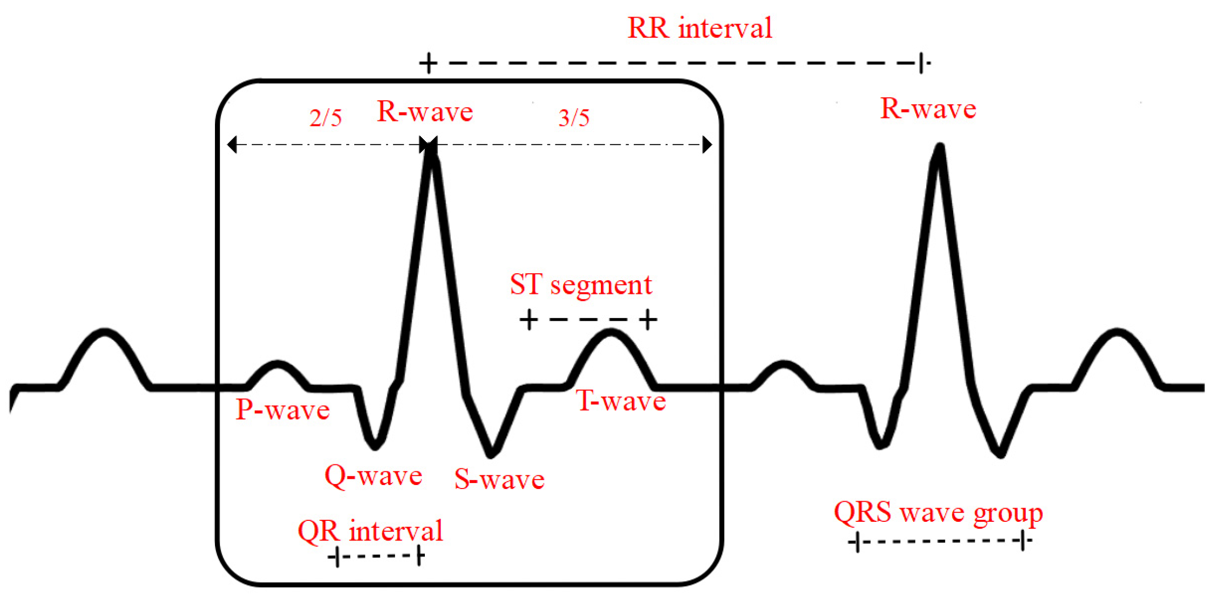
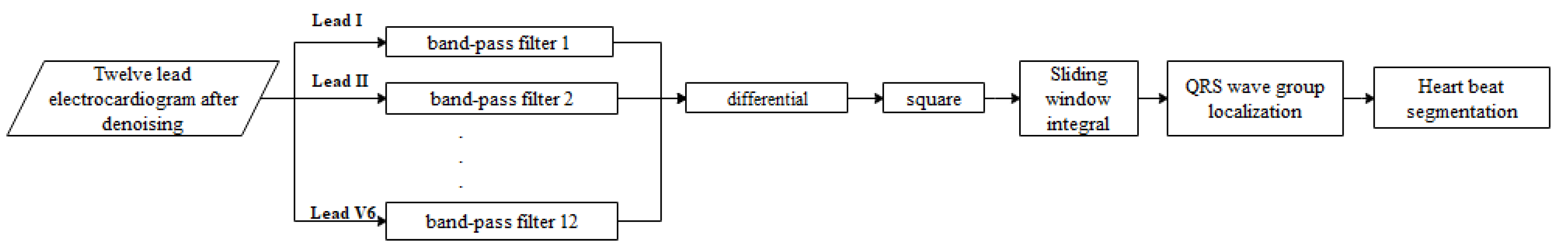
3.4. QRS Wave Group Detection and Heartbeat Segmentation

QRS is the term for electrocardiogram. A heartbeat, a complete impulse of the heart, results in a series of electrical activities, including the depolarization and repolarization of the atria and ventricles, which are denoted by the letters P-QRS-T in electrograms. QRS refers to the whole process of ventricular depolarization. The first downward wave is called the Q wave, the first upward wave is called the R wave, and the second downward wave is called the S wave. The heartbeat of an ECG signal generally consists of the P wave, the QRS wave group, and the T wave, as shown in Figure 4.

The optimized classical Pan–Tompkins (PT) algorithm [13] was applied to locate and segment the 12-lead ECG data into QRS wave clusters and heartbeats. The algorithm flow chart is shown in Figure 5. Because different leads and different myocardial infarction diseases have different QRS complex shapes, different band-pass filters are used to process the ECG signals for different leads, and differential, square, and integral operations are subsequently carried out. Finally, the QRS complex is accurately located in order to carry out accurate beat segmentation.

The R-wave occupies the first 2/5 of a heartbeat, as shown in Figure 4. After the QRS wave group was located, the heartbeat segmentation was performed by taking the R-wave position as a reference and intercepting the ECG signal in the corresponding ratio of front and back.

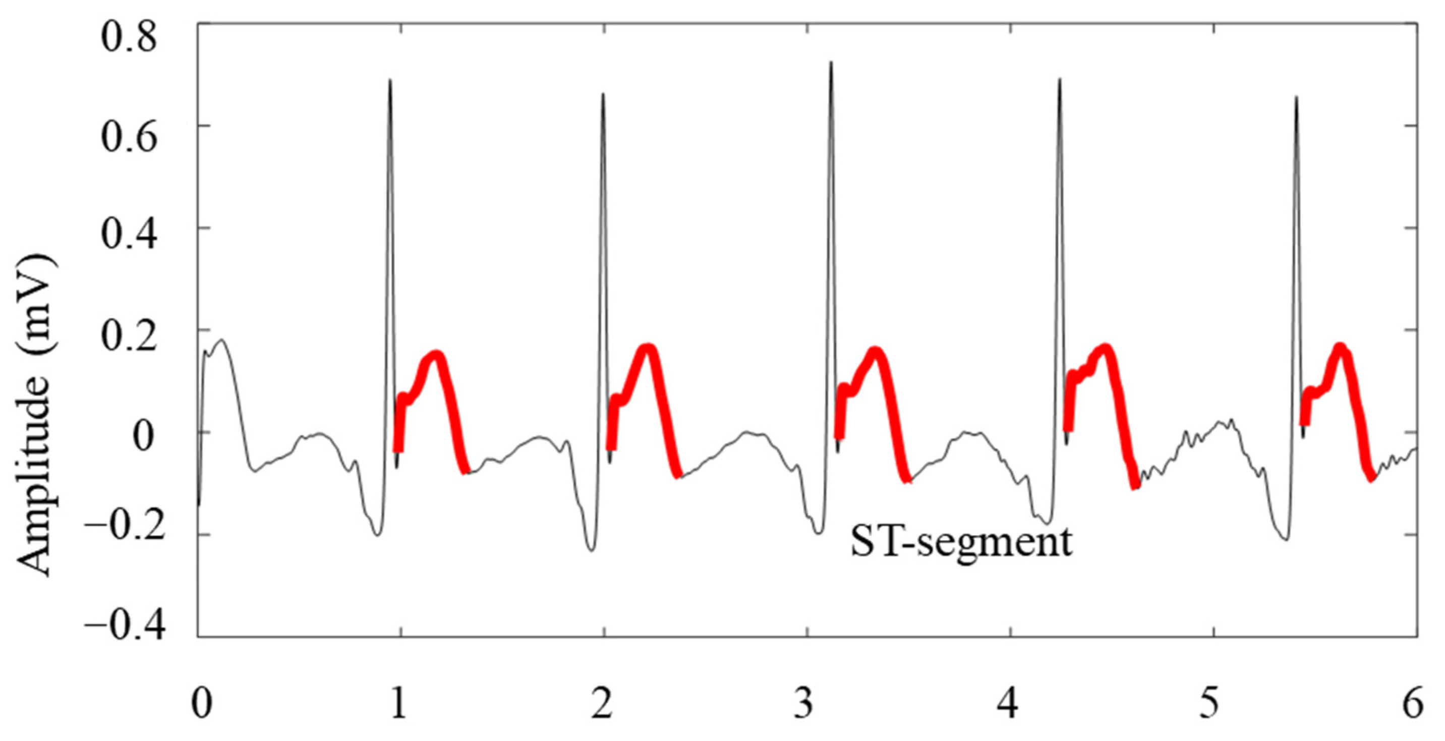
3.5. Amplitude and Distance Feature Extraction of Waveforms

According to the definition in the clinical medical guidelines for cardiology [15], the infarct can be identified as anterior inferior, anterior, anterior interstitial, and anterior lateral, depending on the location of the infarct (culprit vessel), among which inferior and anterior infarcts are common locations in clinical practice. To locate an infarction with ECG, the main method used is to observe the leads in which the necrotic waveforms appear. The necrotic waveform consists of three main categories [16]:

(1)

Pathological Q waves appear on the leads oriented towards the area of myocardial necrosis;

(2)

Injury-type ST-segment elevation appears on leads oriented towards the area of myocardial injury surrounding the area of necrosis;

(3)

T-wave inversion appears on leads oriented towards the area of ischaemia surrounding the area of injury.

Distinct locations of the culprit vessel of myocardial infarction produce projections on different leads. To clearly illustrate this aspect, it is summarized in

Table 2. Electrocardiographic diagnosis of myocardial infarction.

Lead	Inferior	Anterior	Anterior Septal	Anterior Lateral	Inferior Lateral
V1	−	±	+	−	−
V2	−	±	+	−	−
V3	−	+	±	−	−
V4	−	+	−	+	−
V5	−	−	−	+	−
V6	−	−	−	+	−
I	−	−	−	−	+
II	+	−	−	−	−
III	+	−	−	−	−
AVR	−	−	−	−	−
AVL	−	−	−	−	+
AVF	+	−	−	−	−

. Table 2 displays the association between the infarct location and the leads. The symbol “±” indicates that a necrotic waveform may occur in the lead, the symbol “+” indicates that a necrotic waveform will occur in the lead, and the symbol “−” indicates that a necrotic waveform will not occur in the lead. ECG localization is generally consistent with the findings of pathological autopsy.

Therefore, after localization by R-wave, the Q-wave, R-wave, and S-wave were localized primarily by mathematical morphology through a series of multi-valued transformations that processed changes in the slope, positive and negative amplitude peaks and valleys of the signal according to morphological characteristics, and before and after finding the valleys of the Q-wave and S-wave [17]. Using an example of a 12-lead ECG showing inferior wall myocardial infarction disease in the AVF lead, the waveform localization results are shown in Figure 6.

The heartbeat ST segment was obtained according to the ST segment potential measurement point location method used by Ana et al. [18], which has been widely applied. The calculation formula is as follow.

$$X_{ST\left(i\right)}=X_R+0.04\times f_s+0.13\sqrt{\frac{T_{R{R}_i}}{10}\times f_s}$$

(6)

where $X_{ST\left(i\right)}$refers to the initial measurement point of the ST segment, $X_R$refers to the coordinate position of the R-wave crest, $f_s$is the sampling frequency of the overall ECG signal, and $T_{R{R}_i}$ is the RR interval of the overall ECG signal.

The ST segment extraction of the AVF leads in the case above is shown in Figure 7.

In summary, the following effective features were extracted for each heartbeat of the 12-lead ECG, as shown in

Table 3. Description of feature extraction.

Characteristic Type	Characteristic Description	Characteristic Representation
Overall waveform distance characteristics	RR interval	$T_{RR}$
	QR interval	$T_{QR}$
	ST segment potential starting point	$X_{ST}$
12-lead waveform amplitude characteristics	Q-wave amplitude: 12 leads	$V_{Q_{V1}},V_{Q_{V2}},V_{Q_{V3}},V_{Q_{V4}},V_{Q_{V5}},V_{Q_{V6}},V_{Q_I},V_{Q_{II}},V_{Q_{III}},V_{Q_{AVR}},V_{Q_{AVL}},V_{Q_{AVF}}$
	R-wave amplitude: 12 leads	$V_{R_{V1}},V_{R_{V2}},V_{R_{V3}},V_{R_{V4}},V_{R_{V5}},V_{R_{V6}},V_{R_I},V_{R_{II}},V_{R_{III}},V_{R_{AVR}},V_{R_{AVL}},V_{R_{AVF}}$

.

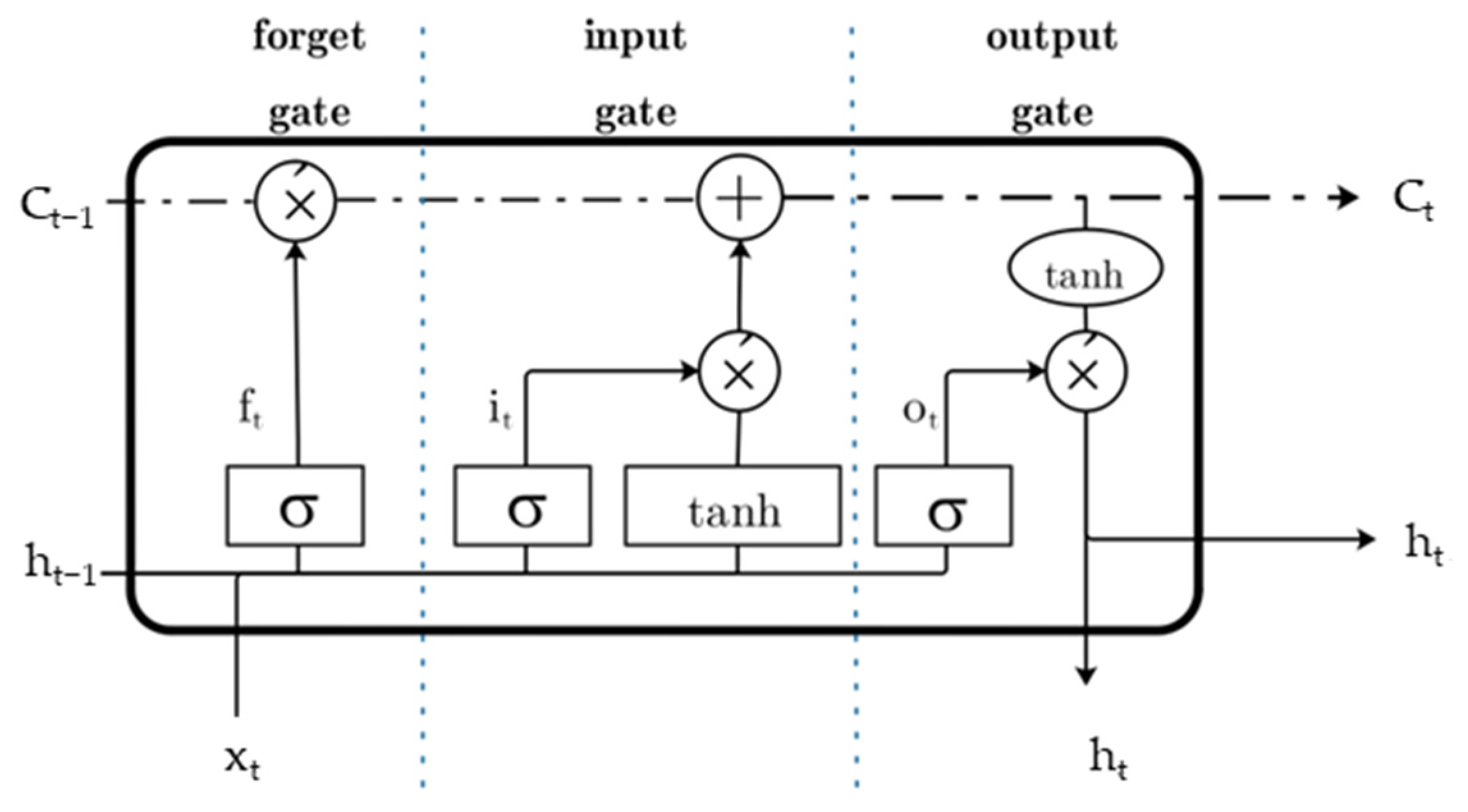
4. Network Structure Modeling

This section introduces the model built in this study. The model is mainly composed of an LSTM cell. Recently, long short-term memory network (LSTM) models have been frequently applied in several fields, such as natural language processing, computer visualization, etc. For temporal structured data, time-varying nonlinear signals, etc., LSTM performs better than other models. LSTM was selected for detection due to specific characteristics, including the time-varying nonlinearity of the ECG signal and the correlation between features [19].

LSTM is structured with the addition of three selectivity modules: forget gate, input gate, and output gate (Figure 8), which control and protect the input information and enable a more adequate filtering of the corresponding features [20].

In Figure 8, the forget gate is controlled by a simple feed-forward neural network to control the forgetting degree of information from the previous time period, as shown in Equation (7).

$$f_t=\sigma \left(W_f\left[x_t,h_{t-1}\right]+b_f\right)$$

(7)

where$x_t$ is the input sequence, and $h_{t-1}$is the output of the previous time module. $W_f$is the weight vector of the forget gate, $b_f$is the corresponding bias vector, and $\sigma$ is a sigmoid function. If the output of the function approaches 0, the cell state of the previous time sequence will be forgotten.

The output variables of the input gate are shown in Equation (8).

$$\begin{gathered} C_t=f_t\times C_{t-1}+i_t\times {\tilde{C}}_t \\ =\sigma \left(W_f\left[x_t,h_{t-1}\right]+b_f\right)\times C_{t-1}+\sigma \left(W_i\left[x_t,h_{t-1}\right]+b_i\right)\times \tan h\left(W_c\left[x_t,h_{t-1}\right]+b_c\right) \end{gathered}$$

(8)

where $C_{t-1}$ is the cell state of the previous time module, and the output variable of the output gate is shown in Equation (9).

$$h_t=\tan h\left(C_t\right)\times o_t=\tan h\left(C_t\right)\times \sigma \left(W_o\left[x_t,h_{t-1}\right]+b_o\right)$$

(9)

The dashed boxes in Figure 8 represent long term memory, while the solid boxes represent short term or working memory.

Based on the LSTM network model, this paper uses the bidirectional LSTM (BiLSTM) network model [21,22] to identify and detect various myocardial infarction diseases. Unlike the traditional LSTM neural network, the input of the network acts on the hidden layers in the front and back directions and then combines the outputs of the two hidden layers to obtain the final output. A schematic diagram of the bidirectional LSTM network structure based on this algorithm is shown in Figure 9.

With the forward and backward networks constructed independently, the output variables of each step in the BiLSTM are joined to form a feature vector, and eventually a fully connected layer is constructed using weight sharing.

5. Results and Discussion

In this section, the experiments and results of the paper are discussed. First, the data composition of the experiment is introduced, and then the verification method of the model is described. Finally, the experimental results are compared and analyzed. The heartbeat dataset used contains a total of 55,212 heartbeats. Data training and model verification are carried out by means of 5-fold cross validation. By dividing the dataset, the practice set accounts for 80%, and the test set accounts for 20%. Then, the training set is divided into a verification set and a training set, according to the 5-fold cross verification method. The specific division of PTB database center beats is shown in

Table 4. Dataset distribution.

Classes	Number of Beats	The Total Training Set (80%)		Number of Beats in Test Set (20%)
		Number of Beats in Training Set (64%)	Number of Beats in Validation Set (16%)
HC	10,483	6661	1666	2156
IMI	11,372	7290	1823	2259
AMI	5571	3590	897	1084
ASMI	10,820	6905	1726	2189
ALMI	6558	4217	1054	1287
ILMI	7408	4752	1188	1468
Total	55,212	33,415	8354	10,443

.

To verify the rationality of the neural network construction, the softmax cross-entropy loss function was used to conduct loss analysis on the practice set and test set, respectively, as shown in Equation (10).

$$E\left(t,y\right)=-{\displaystyle \sum }_j{t}_j\log y_i$$

(10)

where t and y denote the category labels and the actual recognition output values of the neural network, respectively, and $y_i$ denotes the softmax loss function, as shown in Equation (11).

$$y_i=soft\max ax\left(z_j\right)=\frac{e^{zj}}{{{\displaystyle \sum }}_j{e}^{zj}}$$

(11)

In this paper, TensorFlow is used to build the BiLSTM neural network model framework. The network model parameter settings are shown in

Table 5. Network model parameters.

Network Model	BiLSTM
Parameter	Epoch = 400
	Maxiters = 800
	Learining rate = 0.001
	Forget bias = 0.8

.

The training of this model uses an NVIDIA Quadro p2200 graphics card with a 5 g video memory capacity. The training time of the first full epoch of the model is 82S, and then the seconds gradually decrease. The training time of the last 400th epoch reaches 68 s, for a total of 28,911 s, or about 8.03 h.

For classification recognition algorithms, overall accuracy, PPV, and sensitivity are introduced to achieve a better evaluate [23]. The expression formula is as follows in Equations (12)–(16):

$$accuracy=\frac{TP+TN}{TP+TN+FP+FN}\times 100\%$$

(12)

$$sensitivity=\frac{TP}{TP+FN}\times 100\%$$

(13)

$$specificity=\frac{TN}{TN+FP}\times 100\%$$

(14)

$$PPV=\frac{TP}{TP+FP}\times 100\%$$

(15)

$$NPV=\frac{TN}{TN+FN}\times 100\%$$

(16)

where $TP$ denotes the number correctly classified, $FP$ denotes the number of other categories classified into this category, and $FN$ denotes the number of this category incorrectly classified into other categories. The F1-score evaluation index is introduced by combining both evaluation parameters. Since the PPV rate and sensitivity are equally significant, $\beta$takes the value of 1 in the original F1-score calculation formula, which is calculated as follows in Equation (17):

$$F=\frac{2\times precision\times sensitivity}{precision+sensitivity}$$

(17)

The analyses of the loss curve and accuracy (ACC) curve results were performed for the LSTM model and the BiLSTM model, respectively, by selecting the group with the best performance in practice among the 5 sets of practice models using a 5-fold cross-validation, as shown in Figure 10.

From the two loss curves of Figure 10a,c, it can be seen that for the training set and the test set, the two loss curves gradually converge, and the curve does not rise again; the two models finally tend to stabilize, without oscillation. However, the ACC curve of the training set and the test set, shown in Figure 10b,d, indicates that the two models have not reached the over fitting state, and the classification effect is good. The loss curve of the LSTM neural network model in Figure 10a converges relatively slowly, and the accuracy of the final test set is stable at 95.0%, while the loss curve of the BiLSTM neural network model in Figure 10c converges relatively quickly, and the accuracy curve finally stabilizes at 98.6%.

Using the optimal model selected by the 5-fold cross validation to evaluate the test set mutually exclusive with the training set, the confusion matrix is shown in Figure 11; the test results obtained are shown in

Table 6. MI localization results (abbreviations in the table are shown in Table 1).

Model	Label	Accuracy	Sensitivity	Specificity	PPV	NPV	F1-Score
Morphological Feature +LSTM	HC	0.987	0.980	0.989	0.959	0.995	0.969
	IMI	0.979	0.944	0.988	0.958	0.984	0.951
	AMI	0.985	0.923	0.992	0.934	0.991	0.928
	ASMI	0.976	0.941	0.985	0.938	0.985	0.939
	ALMI	0.984	0.938	0.990	0.933	0.991	0.935
	ILMI	0.991	0.965	0.995	0.972	0.994	0.968
	Average	0.984	0.948	0.990	0.949	0.990	0.949
	MI detection (accuracy)	0.950
	kappa	0.939
Morphological Feature +BiLSTM	HC	0.998	0.994	0.999	0.994	0.998	0.994
	IMI	0.994	0.990	0.995	0.981	0.997	0.985
	AMI	0.994	0.984	0.995	0.959	0.998	0.971
	ASMI	0.993	0.972	0.998	0.993	0.993	0.982
	ALMI	0.996	0.980	0.998	0.984	0.997	0.982
	ILMI	0.998	0.994	0.998	0.990	0.999	0.992
	Average	0.996	0.985	0.997	0.984	0.997	0.985
	MI detection (accuracy)	0.986
	kappa	0.983

.

According to the confusion matrix, the recognition accuracy of MI detection can be calculated; that is, the accuracy of only identifying health and myocardial infarction diseases is shown in Equation (18):

$$\mathrm{MI}\mathrm{detection}\left(\mathrm{accuracy}\right)=\frac{HC\left(TP\right)}{HC\left(TP+TN+FP+FN\right)}\times 100\%$$

(18)

According to the above formula, the recognition accuracy of MI detection based on the morphological feature + LSTM algorithm is 97.4%, and the recognition accuracy of MI detection based on the morphological feature + LSTM algorithm is 99.4%.

In order to check the consistency of the algorithm, the kappa ($k$) coefficient is proposed. The calculation formula is as follows in Equations (19)–(21).

$$p_0={{\displaystyle \sum }}_{i=1}^C{T}_i/n$$

(19)

$$p_e=\left({{\displaystyle \sum }}_{i=1}^C{a}_i\times b_i\right)/n^2$$

(20)

$$k=\left(p_0-p_e\right)/\left(1-p_e\right)$$

(21)

where $p_0$ is the sum of the number of correctly classified samples in each class divided by the total number of samples. $C$ is the total number of categories, and $t_i$ is the number of correctly classified samples for each category. $a_i$ is the number of real samples in each category; $b_i$ is the predicted number of samples in each category. According to kappa’s calculation formula, the more unbalanced the confusion matrix, the higher $p_e$, and the lower kappa value.

Specific multiple myocardial infarction diseases and the identification results of culprit vessel location are shown in Table 6.

It can be seen from Table 6 that the recognition rate of the morphological feature +LSTM algorithm in the AMI, ASMI, and ALMI regions is low, but the BiLSTM neural network built in this paper better solved this problem. The recognition accuracy of the morphological feature +BiLSTM algorithm in MI detection reached 99.4%. At the same time, among the six common myocardial infarction diseases, the localization and recognition rate of the culprit vessels is high. The sensitivity and F1 score parameters were greater than 98.4%, while the overall accuracy reached 98.6%, which is 3% higher than the overall recognition accuracy (ACC) of the morphological feature +LSTM algorithm. Meanwhile, the kappa coefficient also reached 0.983. It can be seen that the model has a high degree of balance and does not present the shortcoming of model bias. By reason of the foregoing, the morphological feature +BiLSTM algorithm can well learn the detailed features of the various waveforms of different myocardial infarction diseases.

It can be seen from

Table 7. Comparison of myocardial infarction recognition algorithms.

Author, Year	Methodology	Results
Dohare et al., 2018 [7]	PCA+SVM	MI Detection: Acc = 96.66%; sensitivity = 96.6%
Safdarian N., 2014 [24]	ANN, PNN, KNN, Multilayer perceptron classification	MI Localization: Acc = 76%
Acharya et al., 2017 [25]	CNN	MI Detection: Acc = 95.22%; sensitivity = 95.49%,
Sharma L. D., 2018 [26]	T-wave feature + Naive Bayes	MI Detection: Acc = 94.74% MI Localization: Acc = 76.67%
Proposed method	Morphological Feature + LSTM	MI Detection: Acc = 97.4% MI Localization: Acc = 95.0%; sensitivity = 94.8%
Proposed method	Morphological Feature + BiLSTM	MI Detection: Acc = 99.4% MI Localization: Acc = 98.6%; sensitivity = 98.5%

that the algorithm proposed in this paper can not only better identify the myocardial infarction disease, but also accurately identify the location of criminal angiosclerosis, which presents very important clinical application value.

6. Conclusions

In this paper, an algorithm combining 12-lead morphological features with a BiLSTM network is proposed. Its accuracy reaches 98.6%, and the five parameters—sensitivity, specificity, PPV, NPV, and F1 score—all reach more than 98.4%. Meanwhile, the kappa coefficient also reached 0.983. Compared with other myocardial infarction recognition algorithms, this algorithm has achieved high accuracy in the intelligent recognition of five different elements of myocardial infarction diseases. This study can greatly improve the efficiency of clinical diagnosis and avoid the shortcomings of the existing process, such as being time-consuming and not providing results in a timely manner. This intelligent diagnosis method can effectively reduce the diagnosis time of myocardial infarction, greatly shorten the clinical diagnosis time, save patients’ lives, and conserve medical human resources, to a certain extent. Based on the research in this paper, we will consider adding data from different databases to improve and verify the robustness of this algorithm for disease data testing. On the basis of ensuring the accuracy of the algorithm, we will reduce the number of leads, further optimizing this algorithm.

References

1. Go, A.S.; Mozaffarian, D.; Roger, V.L.; Benjamin, E.; Berry, J.D.; Borden, W.B.; Bravata, D.M.; Dai, S.; Ford, E.S.; Fox, C.S.; et al. Heart Disease and Stroke Statistics—2013 Update. Circulation 2013, 127, e6–e245. [Google Scholar] [CrossRef] [PubMed] [Green Version]
2. Desai, U.; Martis, R.J.; Nayak, C.G.; Seshikala, G. Machine intelligent diagnosis of ECG for arrhythmia classification using DWT, ICA and SVM techniques. In Proceedings of the 2015 Annual IEEE India Conference (INDICON), New Delhi, India, 17–20 December 2015; pp. 1–4. [Google Scholar] [CrossRef]
3. Oh, S.L.; Ng, E.Y.K.; Tan, R.S.; Acharya, U.R. Automated beat-wise arrhythmia diagnosis using modified U-net on extended electrocardiographic recordings with heterogeneous arrhythmia types. Comput. Biol. Med. 2019, 105, 92–101. [Google Scholar] [CrossRef] [PubMed]
4. Han, C.S.; Vig, L. Anomaly detection in ECG time signals via deep long short-term memory networks. In Proceedings of the 2015 IEEE International Conference on Data Science and Advanced Analytics (DSAA), St. Etienne, France, 19–21 October 2015; pp. 1–7. [Google Scholar] [CrossRef]
5. Martis, R.J.; Acharya, U.R.; Min, L.C. ECG beat classification using PCA, LDA, ICA and Discrete Wavelet Transform. Biomed. Signal Process. Control 2013, 8, 437–448. [Google Scholar] [CrossRef]
6. Haraldsson, H.; Edenbrandt, L.; Ohlsson, M. Detecting acute myocardial infarction in the 12-lead ECG using Hermite expansions and neural networks. Artif. Intell. Med. 2004, 32, 127–136. [Google Scholar] [CrossRef] [PubMed]
7. Dohare, A.K.; Kumar, V.; Kumar, R. Detection of myocardial infarction in 12 lead ECG using support vector machine. Appl. Soft Comput. 2018, 64, 138–147. [Google Scholar] [CrossRef]
8. Sharma, M.; Tan, R.S.; Acharya, U.R. A novel automated diagnostic system for classification of myocardial infarction ECG signals using an optimal biorthogonal filter bank. Comput. Biol. Med. 2018, 102, 341–356. [Google Scholar] [CrossRef] [PubMed]
9. Jahmunah, V.; Ng, E.Y.K.; Ru, S.; Shu, L.; Rajendra, A.U. Explainable detection of myocardial infarction using deep learning models with Grad-CAM technique on ECG signals. Comput. Biol. Med. 2022, 146, 105550. [Google Scholar] [CrossRef] [PubMed]
10. Wei, B.P.; Ying, A.; Yu, X.G.; Jian, X.W. MCA-net: A multi-task channel attention network for Myocardial infarction detection and location using 12-lead ECGs. Comput. Biol. Med. 2022, 150, 106199. [Google Scholar] [CrossRef]
11. Goldberger, A.L.; Amaral, L.A.N.; Glass, L.; Hausdorff, J.M.; Ivanov, P.C.; Mark, R.G.; Mietus, J.E.; Moody, G.B.; Peng, C.-K.; Stanley, H.E. PhysioBank, PhysioToolkit, and PhysioNet: Components of a New Research Resource for Complex Physiologic Signals. Circulation 2000, 101, E215–E220. [Google Scholar] [CrossRef] [Green Version]
12. Jackson, L.B. Digital Filters and Signal Processing; Kluwer Academic Publishers: Boston, MA, USA, 1989; pp. 76–92. [Google Scholar] [CrossRef]
13. Kong, D.; Zhu, J.; Wu, S.; Duan, C.; Lu, L.; Chen, D. A novel IRBF-RVM model for diagnosis of atrial fibrillation. Comput. Methods Programs Biomed. 2019, 177, 183–192. [Google Scholar] [CrossRef]
14. Xu, W.; He, W.; You, B.; Guo, Y.; Hong, K.; Chen, Y.; Xu, S.; Chen, X. Acute Inferior Myocardial Infarction Detection Algorithm Based on BiLSTM Network of Morphological Feature Extraction. J. Electron. Inf. Technol. 2021, 43, 2561–2568. [Google Scholar] [CrossRef]
15. Roger, V.L. Epidemiology of Myocardial Infarction. Med. Clin. N. Am. 2007, 91, 537–552. [Google Scholar] [CrossRef] [PubMed] [Green Version]
16. Padhy, S.; Dandapat, S. Third-order tensor based analysis of multilead ECG for classification of myocardial infarction. Biomed. Signal Process. 2017, 31, 71–78. [Google Scholar] [CrossRef]
17. Chen, R.; Huang, Y.; Wu, J. Multi-window detection for P-wave in electrocardiograms based on bilateral accumulative area. Comput. Biol. Med. 2016, 78, 65–75. [Google Scholar] [CrossRef]
18. Mincholé, A.; Jager, F.; Laguna, P. Discrimination between ischemic and artifactual ST segment events in Holter recordings. Biomed. Signal Process. 2010, 5, 21–31. [Google Scholar] [CrossRef]
19. Yildirim, O.; Baloglu, U.B.; Tan, R.; Ciaccio, E.J.; Acharya, U.R. A new approach for arrhythmia classification using deep coded features and LSTM networks. Comput. Methods Programs Biomed. 2019, 176, 121–133. [Google Scholar] [CrossRef] [PubMed]
20. Schmidhuber, J. Deep learning in neural networks: An overview. Neural Netw. 2015, 61, 85–117. [Google Scholar] [CrossRef]
21. Salloum, R.; Kuo, C.C. ECG-based biometrics using recurrent neural networks. In Proceedings of the IEEE International Conference on Acoustics, Speech and Signal Processing (ICASSP), New Orleans, LA, USA, 5–9 March 2017; pp. 2062–2065. [Google Scholar] [CrossRef]
22. Sharma, L.D.; Sunkaria, R.K. Myocardial infarction detection and localization using optimal features based lead specific approach. IRBM 2020, 41, 58–70. [Google Scholar] [CrossRef]
23. Acharya, U.R.; Fujita, H.; Sudarshan, V.K.; Oh, S.L.; Adam, M.; Koh, J.E.W.; Tan, J.H.; Ghista, D.N.; Martis, R.J.; Chua, C.K.; et al. Automated detection and localization of myocardial infarction using electrocardiogram: A comparative study of different leads. Knowl. Based Syst. 2016, 99, 146–156. [Google Scholar] [CrossRef]
24. Safdarian, N.; Dabanloo, N.J.; Attarodi, G. A new pattern recognition method for detection and localization of myocardial infarction using T-Wave integral and total integral as extracted features from one cycle of ECG signal. J. Biomed. Sci. Eng. 2014, 2014, 818–824. [Google Scholar] [CrossRef] [Green Version]
25. Acharya, U.R.; Fujita, H.; Oh, S.L.; Hagiwara, Y.; Tan, J.H.; Adam, M. Application of deep convolutional neural network for automated detection of myocardial infarction using ECG signals. Comput. Biol. Med. 2018, 100, 270–278. [Google Scholar] [CrossRef] [PubMed]
26. Sharma, L.D.; Sunkaria, R.K. Inferior myocardial infarction detection using stationary wavelet transform and machine learning approach. Signal Image Video Process. 2018, 12, 199–206. [Google Scholar] [CrossRef]
Figure 1. Algorithm flow diagram.
Processes 10 02348 g001
Figure 2. Comparison diagram of the signal information entropy of two examples.
Processes 10 02348 g002
Figure 3. Schematic diagram of the ECG signal: (a) original; (b) after de-noising.
Processes 10 02348 g003
Figure 4. Schematic diagram of a standard heartbeat.
Processes 10 02348 g004
Figure 5. Block diagram of the QRS complex location and beat segmentation algorithm, with separate leads [14].
Processes 10 02348 g005
Figure 6. Localization results of the Q wave, R wave, and S wave of the AVF lead in patients with inferior myocardial infarction.
Processes 10 02348 g006
Figure 7. ST segment localization in patients with inferior myocardial infarction.
Processes 10 02348 g007
Figure 8. Schematic diagram of LSTM-cell model structure module.
Processes 10 02348 g008
Figure 9. Schematic diagram of the bidirectional LSTM (BiLSTM) network structure.
Processes 10 02348 g009
Figure 10. The loss curve and ACC curve of the LSTM and BiLSTM neural networks: (a) loss curve of LSTM neural network; (b) ACC curve of LSTM neural network; (c) loss curve of BiLSTM neural network; (d) ACC curve of BiLSTM neural network.
Processes 10 02348 g010
Figure 11. Confusion matrix. (a) LSTM. (b) BiLSTM.
Processes 10 02348 g011