Risk Measures and Portfolio Optimization

Abstract

In this paper we investigate portfolio optimization under Value at Risk, Average Value at Risk and Limited Expected Loss constraints in a continuous time framework, where stocks follow a geometric Brownian motion. Analytic expressions for Value at Risk, Average Value at Risk and Limited Expected Loss are derived. We solve the problem of minimizing risk measures applied to portfolios. Moreover, the portfolio’s expected return is maximized subject to the aforementioned risk measures. We illustrate the effect of these risk measures on portfolio optimization by using numerical experiments.

1. Introduction

A rational investor’s intent is to maximize return while minimizing risk. Under this concept, portfolio theory was developed by Markowitz [1]. Portfolio theory can be simply defined as, the use of decision-making tools to solve the problem of managing risky investment portfolio (see Nawrocki [2]). Some of the basic building blocks of modern portfolio theory is the mean-variance efficiency frontier of Markowitz [3] and the reward-to-variability ratio of Sharpe [4]. Using these major concepts various papers have been developed in continuous time models. Let us mention only a few. Duffie et al. [5] provides a closed form solution for the optimal continuous-time future hedging policy under various mean-variance and quadratic objectives, in an incomplete market. Zhou et al. [6] considers the continuous-time mean-variance model modulated by Markov chain representing the regime switch. Xie et al. [7] investigates portfolio selection with liability in an incomplete financial market. Jewel et al. [8] invokes the delta-gamma approximation to reduce a well-posed quadratic programming problem under a mean-variance framework.

Risk measures in a continuous model are generally difficult to compute due to the myriads of distributions for the gains/losses. There are two main approaches to measuring risk in this setting. The first approach is to use static risk measures (see Emmer et al. [9] and Basak et al. [10]). The second approach is to employ dynamic risk measures (see Cuoco et al. [11], Pirvu et al. [12], Pirvu et al. [13] and Pirvu et al. [14]).

In measuring risk, one observation is that investor’s view of risk is asymmetric about the mean. Hence downside risk measures were introduced. Some common downside risk measures are value at risk, average value at risk and limited expected loss. Value at Risk (VaR) estimates the loss of a portfolio over a given time period with a particular confidence interval. One advantage of VaR is that it is simple to estimate, however “there is a risk in the value at risk itself”, according to Jorion [15]. To address the shortcomings of VaR coherent risk measure were introduced; an example is Average Value at Risk (AVaR) (see Artzner et al. [16]). The AVaR at tail probability α is defined as the average of the VaR’s which are larger than the VaR at tail probability α. It captures what VaR ignores, which is the information on how much one can loose on average if the one goes beyond the VaR confidence level (see Rachev [17]). Limited Expected Loss (LEL) was proposed by Basak and Shapiro [10] and is a variant of AVaR computed under a risk neutral probability measure.

The approach pioneered by Emmer et al. [9] and Basak et al. [10] was considered by many papers. One example is Dmitra$\check{\text{s}}$inovi$\acute{\text{c}}$-Vidovi$\acute{\text{c}}$ et al. [18], where the risk measure used are Value at Risk (VaR), Relative Value at Risk (RVaR) and Capital at Risk (CaR). The corresponding maximal expected return is derived and compared.

In this paper, we follow the approach of Dmitra$\check{\text{s}}$inovi$\acute{\text{c}}$-Vidovi$\acute{\text{c}}$ et al. [18] and Dmitra$\check{\text{s}}$inovi$\acute{\text{c}}$-Vidovi$\acute{\text{c}}$ et al. [19]. The stocks follow a geometric Brownian motion (GBM) process. Risk-reward criterion is utilized with various risk measures. Model parameters are deterministic throughout the paper. Borrowing of the bond is allowed and unconstrained.

Our contribution is to provide explicit formulas for Average Value at Risk (AVaR) and Limited Expected Loss (LEL) risk measures in a geometric Brownian motion model for the risky assets. We further implement and analyse portfolio optimization based on the risk measures aforementioned. Our paper considers a model with continuous distribution hence AVaR and Conditional Value at Risk (CVaR) are the same (see Follmer et al. [20]). The portfolio optimization problem involves the risk-reward criterion. We apply a dimension reduction technique to transform the m-dimensional optimization problem into a 1-dimensional problem which is solved in closed form or numerically. Our paper contains the formulas for VaR, AVaR, LEL and expected wealth. Secondly, we drive expressions for the minimal VaR, AVaR and LEL. We prove that minimizing VaR, AVaR and LEL under an expected return constraint produces the same optimal strategy. We maximize expected wealth with VaR, AVaR, and LEL constraints. For each optimization problem considered the optimal strategy obtained is unique. Numerical experiments show that the most conservative risk constraint is LEL, followed by AVaR and VaR. However, on the critical side LEL is computed under a risk neutral measure thus underestimating stocks returns, and VaR ignores the losses beyond the confidence threshold α. AVaR on the other hand captures all the attributes that the aforementioned risk measures ignore, hence considered to be the best risk measure. The results further show the effect of diversification. The intuitive knowledge that the volatility of the stock is inversely related to the attractiveness of the stock is confirmed. Furthermore, the result exhibit that the confidence threshold has a strong effect on downside risk measures. Various efficient frontiers are illustrated and confirm that the more risk one takes the higher the expected return.

The outline of this paper is as follows: Section 2 contains the model; optimization problems are in Section 3 with the numerical results in Section 4. The appendix contains all the mathematical proofs.

Notations: The following notations apply throughout this paper.

• The m-dimensional column vectors with each component equal to 1 is denoted by $\mathbf{1}$.
• The Euclidean norm of a matrix or vector is denoted by $\left|\right|.\left|\right|$. The $L^2([0,T],{\Re }^n)$ denotes the set of ${\Re }^n$-valued, square-integrable functions defined on $[0,T]$, with its natural inner product ${\langle f,g\rangle }_t={\sum }_{i=1}^n{\int }_0^t{f}_i\left(s\right)g_i\left(s\right)ds.$ Here ${\left|\right|f\left|\right|}_t=\sqrt{{\langle f,f\rangle }_t}$ is the corresponding norm.
• ${\pi }_c$ denotes the area of a circle with radius 1.

2. The Model

Consider a probability space $(\Omega ,{\left\{{\mathcal{F}}_t\right\}}_{0\le t\le T},\mathcal{F},P),$ which accommodates a standard multidimensional Brownian motion. Moreover, consider a financial market model with the following specification:

• One asset is invested in the money market. The money market is represented by $S_0\left(t\right)$,

  $$\frac{d{S}_0\left(t\right)}{S_0\left(t\right)}=r\left(t\right)dt\text{and}R\left(t\right)=exp\left({\int }_0^{t}r\left(s\right)ds\right)$$

  (1)

  The interest rate denoted by $r\left(t\right)$ is deterministic.
• Assets are traded continuously over a finite time horizon $[0,T]$ in a frictionless market.
• m assets are traded in the stock which follow a geometric Brownian motion, i.e.,

  $$d{S}_i\left(t\right)=S_i\left(t\right)\left(b_i\left(t\right)dt+\sum _{j=1}^m{\sigma }_{ij}\left(t\right)d{W}^j\left(t\right)\right).$$

  ${\left({\sigma }_{ij}\left(t\right)\right)}_{i,j=1,...m}$ is deterministic and denotes an invertible volatility matrix; $b_i\left(t\right)$ is deterministic and denotes the drift of the stock, $b\left(t\right)={(b_1\left(t\right),...,b_m\left(t\right))}^{\prime }$. $W\left(t\right)={\left(W^j\left(t\right)\right)}_{j=1,..m}$ is a m-dimensional Brownian motion and $0<r\left(t\right)<b_i\left(t\right)$. Drift and volatility functions are square-integrable.
• Number of shares of asset i held in the portfolio is denoted by $N_i\left(t\right)$. The fraction of wealth $X\left(t\right)$ invested in the risky stock i is denoted by ${\pi }_i\left(t\right)=\frac{N_i\left(t\right)S_i\left(t\right)}{X\left(t\right)}.$$\pi \left(t\right)={({\pi }_1\left(t\right),...,{\pi }_m\left(t\right))}^{\prime }\in {\Re }^m$ is deterministic.
• $\alpha \in (0,0.5)$, denotes the confidence level.

Under the risk neutral probability measure denoted $Q,$ the stock dynamics is

$$dS\left(t\right)=r\left(t\right)S\left(t\right)dt+\sigma \left(t\right)d\tilde{W}\left(t\right)$$

(2)

Here $\tilde{W}\left(t\right)$ denotes the Brownian motion under Q.

The investor invests $\pi \left(t\right)$ in the risky stock and $1-\pi \left(t\right)$ in the bond. The initial wealth $X\left(0\right)$ is positive. The wealth follows a self-financing strategy, hence

$$dX\left(t\right)=X\left(t\right)((r\left(t\right)+B{\left(t\right)}^{\prime }\pi \left(t\right))dt+\sigma {\left(t\right)}^{\prime }\pi \left(t\right)dW\left(t\right))$$

(3)

where $B\left(t\right):=b\left(t\right)-r\left(t\right)\mathbf{1}.$ Thus

$$X\left(t\right)=X\left(0\right)exp\left({\int }_0^t{(r\left(s\right)+B\left(s\right)}^{\prime }\pi \left(s\right)-\frac{1}{2}{\left|\right|\sigma \left(s\right)}^{\prime }{\pi \left(s\right)\left|\right|}^2)ds+{\int }_0^t{\left|\right|\sigma \left(s\right)}^{\prime }\pi \left(s\right)\left|\right|dW\left(s\right)\right)$$

(4)

3. Portfolio Optimization with Risk Constraints

In this section various optimization problems are considered.

3.1. Risk Measures

The various risk measures are considered in this section. They are applied to a loss process defined by

$$Loss\left(t\right)=X\left(0\right)-X\left(t\right)$$

3.1.1. Value at Risk (VaR)

Let us begin with a formal definition.

Definition 3.1.1.1 Value at Risk is the maximum amount of wealth one can likely lose over a period at a specific confidence level α.

$$Va{R}_{\alpha }\left(Loss\left(t\right)\right)=inf\left\{m\right|P(Loss\left(t\right)\le m)\ge 1-\alpha \}$$

This means that with $\alpha =5\%$ there is a $95\%$ probability that the loss will not exceed $Va{R}_{\alpha }\left(Loss\left(t\right)\right)$. In other words there is a $5\%$ probability that the loss can exceed $Va{R}_{\alpha }\left(Loss\left(t\right)\right)$.

Proposition 3.1.1.1 It follows from direct computations that

$$\begin{array}{ccc}\hfill Va{R}_{\alpha }\left(Loss\left(t\right)\right)& =& X\left(0\right)(1-R\left(t\right)exp({\int }_0^t{(B\left(s\right)}^{\prime }\pi \left(s\right)-\frac{1}{2}{\left|\right|\sigma \left(s\right)}^{\prime }{\pi \left(s\right)\left|\right|}^2)ds\hfill \\ \mathrm{(5)}& & +& \left(N^{-1}\left(\alpha \right)\right)\sqrt{{\int }_0^t{\left|\right|\sigma \left(s\right)}^{\prime }\pi \left(s\right){\left|\right|}^{2}ds}\left)\right)\hfill \end{array}$$

Proof of Proposition 3.1.1.1: See appendix A.1.

3.1.2. Average Value at Risk-(AVaR)

Let us begin with a formal definition (see Follmer et al. [20]).

Definition 3.1.2.1 The Average Value at Risk is

$$AVa{R}_{\alpha }\left(Loss\left(t\right)\right)=\frac{1}{\alpha }{\int }_0^{\alpha }Va{R}_u\left(Loss\left(t\right)\right)$$

Proposition 3.1.2.1 It follows from direct computations that

$$\begin{array}{ccc}\hfill AVa{R}_{\alpha }\left(Loss\left(t\right)\right)& =& X\left(0\right)(1-\frac{R\left(t\right)}{\alpha }(exp{\int }_0^{t}B{\left(s\right)}^{\prime }\pi \left(s\right)ds\hfill \\ \mathrm{(6)}& & +& ln\left(N\left(N^{-1}\left(\alpha \right)-\sqrt{{\int }_0^t{\left|\right|\sigma \left(s\right)}^{\prime }\pi \left(s\right){\left|\right|}^{2}ds}\right)\right))\hfill \end{array}$$

Proof of Proposition 3.1.2.1: See appendix A.2

3.1.3. Limited expected loss measure

Let us begin with a formal definition.

Definition 3.1.3.1 The LEL is defined by

$$LE{L}_{\alpha }\left(Loss\left(t\right)\right)=\frac{1}{\alpha }{\int }_0^{\alpha }Va{R}_u^Q\left(Loss\left(t\right)\right)du$$

where $Va{R}_u^Q$ is the VaR evaluated under the risk neutral probability measure $Q.$

Proposition 3.1.3.1 It follows from direct computations that

$$\begin{array}{ccc}\hfill LE{L}_{\alpha }\left(Loss\left(t\right)\right)& =& X\left(0\right)\left(1-\frac{R\left(t\right)}{\alpha }\left(N\left(N^{-1}\left(\alpha \right)-\sqrt{{\int }_0^t{\left|\right|\sigma \left(s\right)}^{\prime }\pi \left(s\right){\left|\right|}^{2}ds}\right)\right)\right)\hfill \end{array}$$

(7)

Proof of Proposition 3.1.3.1 See appendix A.3

3.2. Portfolio Optimization by Minimizing Risk Measures

We restrict to the class of admissible portfolio $\pi (·)$ which are Borel measurable, deterministic and bounded over $[0,T]$. We denote by Q the set of admissible portfolio. The market price of risk is denoted by

$$\theta \left(t\right)=\sigma {\left(t\right)}^{-1}B\left(t\right)$$

(8)

In this section the optimization problem considered is

$$\left(A1\right)\underset{\pi \in Q}{min}\left[RM\left(Loss\right(T\left)\right)\right],\text{where}RM\in \{VaR,AVaR,LEL\}$$

Theorem 3.2.1 Set

$${\left|\right|\Theta \left|\right|}_T:=\sqrt{{\int }_0^T{\left|\right|\sigma \left(t\right)}^{-1}B\left(t\right){\left|\right|}^{2}dt}$$

(9)

The optimal strategy for (A1) is

$${\pi }_{{\epsilon }_{*}}\left(t\right)=\frac{{\epsilon }_{*}}{{\left|\right|\Theta \left|\right|}_T}{\left(\sigma \left(t\right)\sigma {\left(t\right)}^{\prime }\right)}^{-1}B\left(t\right),t\in [0,T]$$

(10)

Here ${\epsilon }_{*}$ is a positive constant and it depends on the risk measure under consideration (see appendix A.4).

3.3. Portfolio Optimization by Minimizing Risk subject to Expected Return Constraint

In this section we minimize risk subject to expected return constraint.

$$\left(A2\right)\underset{\pi \in Q}{min}\left[RM\left(Loss\right(T\left)\right)\right]\text{subject}\text{to}E\left(X\left(T\right)\right)=M$$

Here $RM\in \{VaR,AVaR,LEL\}$ and M is a constant. It is further assumed that $M>X\left(0\right)R\left(T\right)$.

Theorem 3.3.1 Let

$$\zeta =ln\left(\frac{M}{X\left(0\right)R\left(T\right)}\right)$$

(11)

The optimal strategy for (A2) is

$${\pi }_{*}\left(t\right)=\frac{\zeta }{{\left|\right|\Theta \left|\right|}_T^2}{\left(\sigma \left(t\right)\sigma {\left(t\right)}^{\prime }\right)}^{-1}B\left(t\right)$$

(12)

Thus, the optimal strategy is the same for all the risk measures in (A2). See appendix A.5.

3.4. Portfolio Optimization by Maximizing Expected Wealth with Risk Constraints

In this section the expected wealth is maximized while constraining the risk measures.

$$\left(A3\right)\underset{\pi \in Q}{max}\left[E\left(X\left(T\right)\right)\right]\text{subject}\text{to}$$

$$RM\left(Loss\right(T\left)\right)\le C$$

Here $RM\in \{VaR,AVaR,LEL\}$ and C is a constant. We assume that $0<C<X\left(0\right).$

Theorem 3.4.1 The optimal strategy for (A3) is

$${\pi }_{{\epsilon }_{**}}\left(t\right)=\frac{{\epsilon }_{**}}{{\left|\right|\Theta \left|\right|}_T}{\left(\sigma \left(t\right)\sigma {\left(t\right)}^{\prime }\right)}^{-1}B\left(t\right)$$

(13)

Here ${\epsilon }_{**}$ is a positive constant and depends on the risk measure under consideration (see appendix A.6).

Remark: The two fund separation theorem states that investors who must allocate their wealth between a number of risky assets and the money market should have the same mutual fund of risky assets (see Pirvu et al. [21], Schmedders [22], Merton [23] and Tobin [24]). We can conclude that, the optimal portfolios follow a two fund separation. The optimal investment is attained by investing in the money market and in a market portfolio which is a fixed mixture of the m risky stocks Dmitra$\check{\text{s}}$inovi$\acute{\text{c}}$-Vidovi$\acute{\text{c}}$ et al. [18]. The market portfolio ${\pi }_M\left(t\right)$ is defined as

$${\pi }_M\left(t\right)={\left(\sigma {\left(t\right)}^{\prime }\sigma \left(t\right)\right)}^{-1}B\left(t\right)$$

We have shown that every optimal strategy can be expressed as

$${\pi }_{**}\left(t\right)=\frac{\gamma }{{\left|\right|\Theta \left|\right|}_T}{\pi }_M\left(t\right)$$

4. Numerical Analysis

Here we follow Dmitra$\check{\text{s}}$inovi$\acute{\text{c}}$-Vidovi$\acute{\text{c}}$ et al. [18] and [19]. To keep the exposition simple, the interest rate and the volatility matrix are assumed constant. Three stocks are considered. The drift of the stock i is denoted by $b_i\left(t\right)$, where

$$b_i\left(t\right)=u_i+{\beta }_{i}cos\left({\phi }_{i}t\right)$$

(14)

Here ${\phi }_i$ denotes the economic cycle, $u_i$ denotes the average rate of return and ${\beta }_i$ denotes the deviation around $u_i$. The variance covariance matrix is denoted by $\Gamma \left(t\right)dt,$ and

$$\Gamma \left(t\right)=\sigma \left(t\right)\sigma {\left(t\right)}^{\prime }=v\left(t\right)\rho \left(t\right)v\left(t\right)$$

(15)

where the diagonal matrix $v\left(t\right)$ denotes the standard deviation and $\rho \left(t\right)$ denotes the correlation matrix. We take

$$v\left(t\right)=diag[0.2,0.25,0.3]$$

(16)

and

$$\rho \left(t\right)=\left[\begin{array}{ccc}1.00& -0.60& -0.80\\ -0.60& 1.00& 0.50\\ -0.80& 0.50& 1.00\end{array}\right].$$

The time horizon considered is 8 years and time granularity for the parameters below are yearly. We have $u_1=0.08$, $u_2=0.1$, $u_3=0.12$ and $r=0.05$. Let ${\phi }_1={\phi }_2={\phi }_3=0.75$, ${\beta }_1=0.75\beta ,{\beta }_2=0.5\beta ,{\beta }_3=0.25\beta$ and $\beta =0.015$. Take $C=0.7·X\left(0\right).$

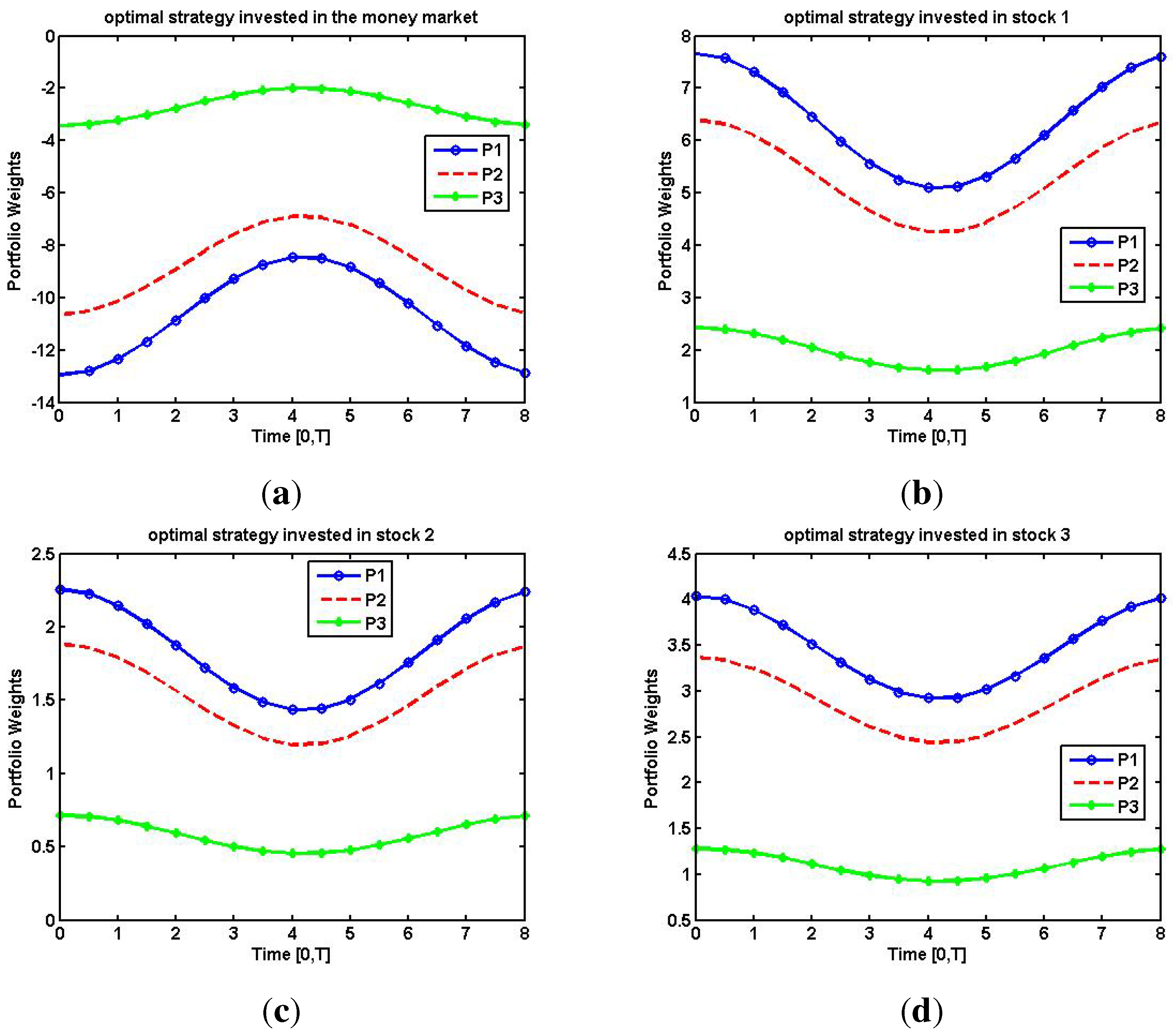
4.1. Optimal Strategy with Risk Constraints

In this section, the optimal strategies for the maximal expected wealth with VaR, AVaR and LEL constraints are considered and illustrated in Figure 1 (b,c,d). The highest portfolio weight is in stock 1 as it is the least volatile. The optimal strategy for stock 1 in P1 is higher than that of P2, followed by P3. See from the footnote that, LEL is the most conservative risk measure, followed by AVaR and VaR. LEL operates under the assumption that the investor is risk neutral. VaR ignores the losses beyond the α threshold. AVaR deals with the disadvantages associated with LEL and VaR, hence is considered to be the best risk measure. Although, stock 3 is more volatile than stock 2, the portfolio weight in stock 3 is higher in stock 2 due to diversification effect introduced by the correlation matrix. The following notation apply: P1 = Maximizing expected return with VaR constraint; P2 = Maximizing expected return with AVaR constraint and P3 = Maximizing expected return with LEL constraint.

Figure 1. (a) Optimal portfolio strategy in the money market (upper left); (b) stock 1 (upper right); (c) stock 2 (lower left) and (d) stock 3 (lower right).

Figure 1. (a) Optimal portfolio strategy in the money market (upper left); (b) stock 1 (upper right); (c) stock 2 (lower left) and (d) stock 3 (lower right).

4.2. Expected Return with Risk Constraints

As illustrated in Figure 2 (a) the maximal expected return occurs in the order P3 followed by P2 and P1. This is intuitive since LEL is the most conservative risk measure compared to AVaR and VaR. The expected return is plotted where $T\in [0,8]$.

Figure 2. (a) Expected return (upper left); (b) Optimal strategy with various confidence levels (upper right).

Figure 2. (a) Expected return (upper left); (b) Optimal strategy with various confidence levels (upper right).

Figure 3. Efficient frontier.

Figure 3. Efficient frontier.

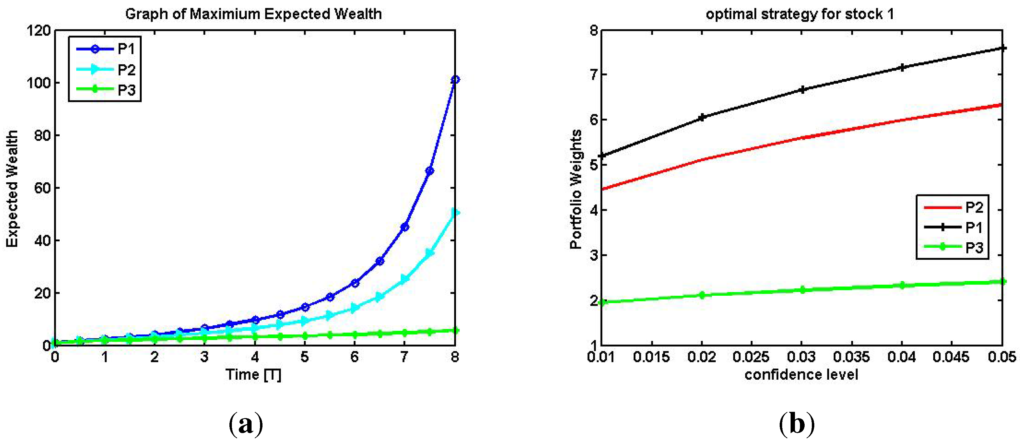
4.3. Optimal Strategy with Different Confidence Interval

In Figure 2(b) the plot shows the optimal strategy in stock 1 for P1, P2 and P3 for the confidence level, $\alpha \in [0.01,0.06]$. As α increases the portfolio weight increases for P1, P2 and P3.

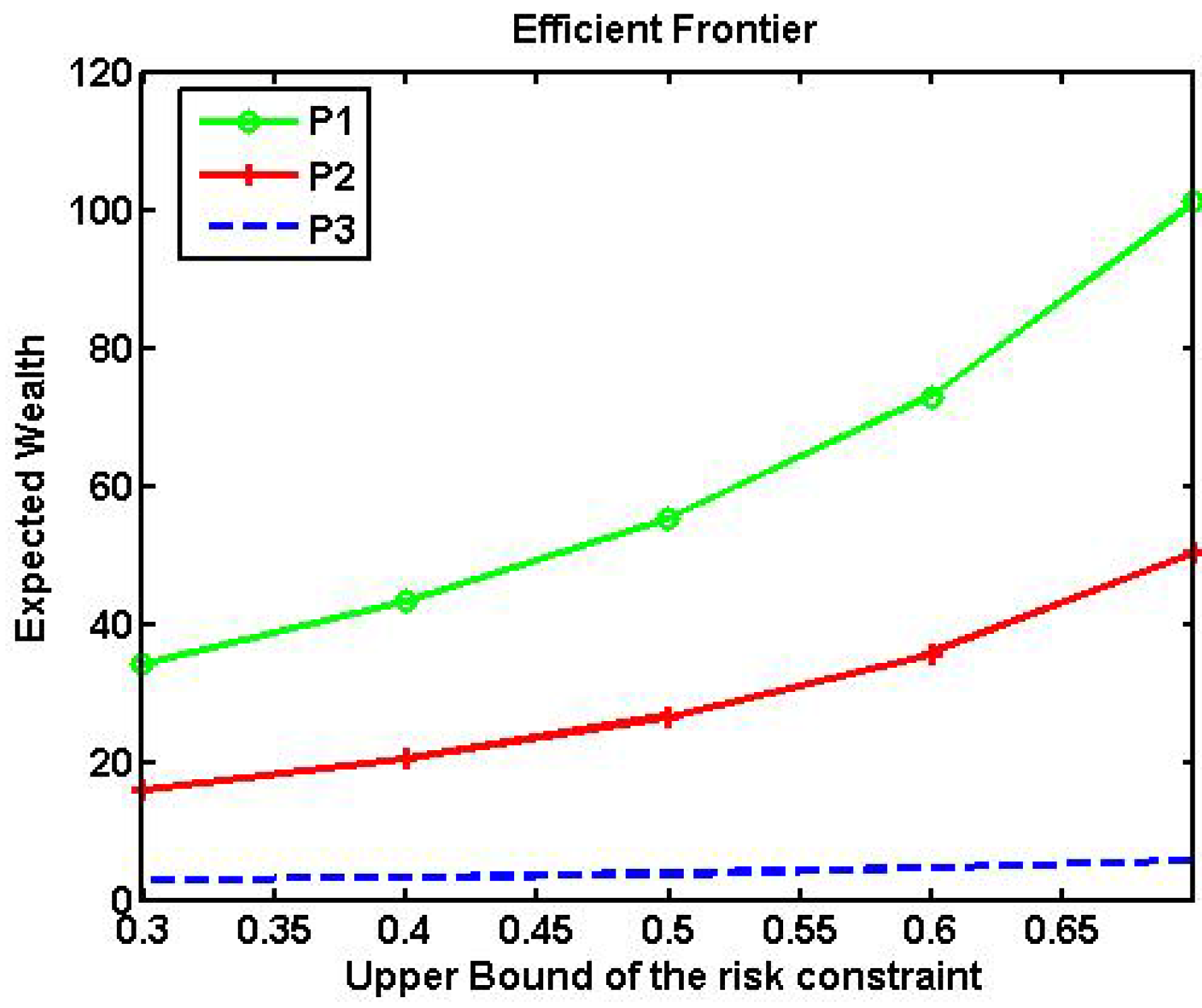
4.4. Efficient Frontier

In Figure 3, we take $C=[0.3,0.7]$. The plot shows that as C increases, the portfolio weights also increase for P1, P2 and P3. The reason being that the higher the risk threshold, the higher the risk appetite of the investor. Hence, the amount invested in the stock increases.

5. Conclusions

In a multiple stock model following a geometric Brownian motion, the VaR, AVaR and LEL risk measures are considered. Furthermore, we maximize expected wealth with VaR, AVaR and LEL constraints, then we find the portfolios which minimizes these risk measure. Using numerical experiments we notice that LEL is the most conservative risk measure, followed by AVaR and VaR.

References

1. H. Markowitz. “Foundation of Portfolio Theory.” J. Financ. 46 (1991): 469–477. [Google Scholar] [CrossRef]
2. D.N. Nawrocki. “A brief history of downside risk measure.” J. Invest. 8 (1999): 9–25. [Google Scholar] [CrossRef]
3. H. Markowitz. “Portfolio Selection.” J. Financ. 7 (1952): 77–91. [Google Scholar]
4. W. Sharpe. “Mutual Fund Performance.” J. Bus. 9 (1966): 119–138. [Google Scholar] [CrossRef]
5. D. Duffie, and H.R. Richardson. “Mean-Variance Hedging in Continuous Time.” Ann. Appl. Probab. 1 (1991): 1–15. [Google Scholar] [CrossRef]
6. X.Y. Zhou, and G. Yin. “Markowitz Mean-Variance Portfolio Selection with Regime Switching: A continuous-time model.” SIAM J. Control Optim. 42 (2003): 1466–1482. [Google Scholar] [CrossRef]
7. S. Xie, Z. Li, and S. Wang. “Continuous-time Portfolio Selection with Liability: Mean-Variance model and Stochastic LQ approach.” Insur.: Math. Econ. 42 (2008): 943–953. [Google Scholar] [CrossRef]
8. S.W. Jewell, Y. Li, and T.A. Pirvu. “Non-linear equity portfolio variance reduction under a mean-variance framework–A delta-gamma approach.” Oper. Res. Lett. 41 (2013): 694–700. [Google Scholar] [CrossRef]
9. S. Emmer, C. Klu¨ppelberg, and R. Korn. “Optimal portfolios with bounded capital at risk.” Math. Financ. 11 (2001): 365–384. [Google Scholar] [CrossRef]
10. S. Basak, and A. Shapiro. “Value-at-risk based management: Optimal policies and Asset Prices.” Rev. Financ. Stud. 14 (2001): 371–405. [Google Scholar] [CrossRef]
11. D Cuoco, H. He, and S. Isaenko. “Optimal Dynamic Trading Strategies with Risk Limits.” Oper. Res. 56.2 (2008): 358–368. [Google Scholar]
12. T.A. Pirvu. “Portfolio Optimization under the Value-at-Risk Constraint.” Quantitat. Financ. 7 (2007): 125–136. [Google Scholar] [CrossRef]
13. T.A. Pirvu, and G. Zˇitkovic´. “Maximizing Portfolio Growth Rate under Risk Constraints.” Math. Financ. 19 (2009): 423–455. [Google Scholar] [CrossRef]
14. S. Moreno-Bromberg, T.A. Pirvu, and A. Reveillac. “CRRA Utility Maximization under Risk Constraints.” Commun. Stoch. Anal. 7 (2013): 203–225. [Google Scholar]
15. P. Jorion. “Measuring the Risk in Value at Risk.” Financ. Anal. J. 52 (1996): 47–56. [Google Scholar] [CrossRef]
16. P. Artzner, F. Delbaen, and J. Eber. “Coherent Measures of Risk.” Math. Financ. 9 (1999): 203–228. [Google Scholar] [CrossRef]
17. T.S. Rachev, V.S. Stoyanov, and J.F. Fabozzi. A Probability Metrics Approach to Financial Risk Measures. West Sussex, UK: Wiley-Blackwell. A John Wiley and Sons Ltd. Publication, 2011, pp. 191–251. [Google Scholar]
18. G. Dmitrasˇinovic´-Vidovic´, and A. Ware. “Asymptotic Behaviour of Mean-Quantile Efficient Portfolios.” Financ. Stoch. 10 (2006): 529–551. [Google Scholar] [CrossRef]
19. G. Dmitrasˇinovic´-Vidovic´, A. Ware, A. Lari-Lavassani, and X. Li. Dynamic Portfolio Selection under Capital-at-Risk. Calgary, Canada: University of Calgary, 2003. [Google Scholar]
20. H. Follmer, and A. Schied. Stochastic Finance: An Introduction in Discrete Time. Chapter 4; Berlin, Germany: Walter de Gruyter, 2004. [Google Scholar]
21. T.A. Pirvu, and K. Schulze. “Multi-Stock Portfolio Optimization under Prospect Theory.” Math. Financ. Econ. 6 (2012): 337–362. [Google Scholar] [CrossRef]
22. K. Schmedders. “Two-fund separation in Dynamic General Equilibrium.” Discuss. Paper//Centre Math. Stud. Econ. Manag. 1398 (2004). [Google Scholar] [CrossRef]
23. R.C. Merton. “An Intertemporal Capital Asset Pricing Model.” Econometrica 41 (1973): 867–887. [Google Scholar]
24. J. Tobin. “Liquidity Preferences as Behavior towards Risk.” Rev. Econ. Stud. 25 (1958): 65–86. [Google Scholar] [CrossRef]