1. Introduction
Before Markowitz [
1] and others, investors concentrated on investment returns but did not think carefully about risk. Markowitz
et al. realized that risk was also an important factor when forming a portfolio and used variance of the return as a first risk measure. They measured past variance of a stock and assumed it would continue into the future. They also found that when stocks are combined into a portfolio, risk can be dramatically reduced. Bad news on one stock may be offset by good news on another stock, reducing variance. After combining about 15–20 stocks into a portfolio the benefits of diversification are mostly exhausted. The investor can no longer significantly decrease risk simply by adding additional stocks. Essentially, the investor is left with market risk, also called non-diversifiable risk. Variance as a measure of risk is no longer adequate because it includes diversifiable risk. A new theory and measure of risk was needed.
In the field of financial economics, the Capital Asset Pricing Model (CAPM) was developed and has been a key theory since the 1960s (see Sharpe [
2] and others). One of its main contributions is to attempt to identify how the risk of a particular stock is related to the risk of the overall stock market. A main measure of this type of risk is called “Beta”. To estimate “Beta”, the returns of a particular stock (
Rit) are regressed on the returns of a stock market proxy, say the S&P 500 (
Rmt):
The estimate of βi is usually obtained using ordinary least squares (OLS) regression. The OLS estimates the responsiveness of Rit to changes in Rmt near the “center” of the distribution and provides an estimate of the average risk for the stock in relation to the risk of the overall market. If the estimated βi is greater than (less than) 1.0, the stock is considered to be riskier (less risky) than the overall market on average and if the βi is close to 1.0, the stock is about equally risky as the market on average.
If the relationship between a stock and the overall market exhibits heteroskedasticity, then more can be learned about the stock’s behavior and its risk characteristics. Heteroskedasticity occurs when the variance of the error term εit varies across different values of Rmt. When the variance of the error term increases (decreases) as the overall market return increases, we call this “diverging (converging) heteroskedasticity”. The quantile regression estimates of the Beta slope under diverging (converging) heteroskedasticity will generally increase (decrease) as we move from the lower towards the upper tail of the Rit distribution. These patterns of heteroskedasticity may provide information useful to investors. Investors may be able to select stocks that exhibit patterns that more closely match their preferences.
Kahneman and Tversky [
3] developed prospect theory which has been used to examine the behavioral aspects of stock market investors. One prediction that is made from their theory is that: (i) People exhibit “loss-aversion” in a gain frame; and (ii) People exhibit “risk-seeking” in a loss frame.
In essence, if a person had done well or “gained”, they tend to be concerned about avoiding losses. Alternatively, if a person has experienced a bad outcome or has “lost”, their behavior may be risk seeking, perhaps trying to get back some of their losses. This implies that investors may prefer riskier stocks (higher Beta) after a down markets (lower stock returns) and less risk (lower Beta) after an up markets (higher stock returns).
There are numerous examples of research that follows a similar line. Investors are shown to demonstrate a strong preference for realizing winners rather than losers (Odean, [
4]). In addition, investors have a general disposition to sell winners too early and hold losers too long (Shefrin and Statman [
5]). This idea is also discussed in (Dacey and Zielonka [
6]). Compared to lottery winners, accident victims take longer to return to their baseline of happiness (Brickman
et al. [
7]). People will do more to avoid a loss than to acquire a comparable gain (Baumeister
et al. [
8]). When investors attempt to avoid the pain of regret by changing the lens through which they view losses, they become more likely to hold onto bad investments (Seiler and Seiler [
9]). Firms with returns above their reference levels take less risk than firms with returns below their reference levels (Kliger and Tsur [
10]).
If a measure can be developed for each stock that incorporates investor’s preferences across good times and bad it could improve our ability to select portfolios that match investor’s preferences. When considering the Beta of a stock, a flatter slope (safer) during good times (higher stock prices
Rit) and steeper slope (more risky) during bad times (lower stock prices
Rit) would match the Kahneman and Tversky [
3] findings. This would lead investors to prefer stocks that exhibit converging rather than diverging heteroskedasticity as will be explained in detail in
Section 4.
In addition, investors may prefer a higher variance of return on their stocks when the market return
Rmt is down and a smaller variance of return on their stocks when the market is up. This also would lead investors to prefer converging rather than diverging heteroskedasticity which again will be explained in
Section 4.
In the following section the data selection process is described. Then a discussion of quantile regressions is presented followed by a discussion of the results and their implications.
3. Quantile Regression
The quantile regression technique invented by Koenker and Bassett [
11] is a very powerful tool in uncovering heteroskedasticity in a regression model. In the CAPM model, given
n observations of the individual return
Rit and the market return
Rmt for
t = 1, …,
n, the
τ-th quantile regression coefficients,
![Jrfm 07 00067 i001]()
and
![Jrfm 07 00067 i002]()
, minimize the following objective function:
where 0 <
τ < 1 determines the desired conditional quantile of interest. In the objective function, the positive and negative residuals,
Rit −
![Jrfm 07 00067 i001]()
−
![Jrfm 07 00067 i002]() Rmt
Rmt, receive different weights in the minimization process. All the positive residuals are assigned a weight of
τ while the negative ones receive a weight of (
τ − 1). Hence, 100
τ% of the individual returns will fall above the
τ-th quantile regression line
![Jrfm 07 00067 i001]()
+
xi ![Jrfm 07 00067 i002]()
and 100(1 −
τ)% below. Hence, the
τ-th quantile regression line bisects the individual returns into two different portions, 100
τ% and 100(1 −
τ)%, conditioned on the various market returns. The special case of the 0.5-th quantile regression line, which is also the median regression line, divides the individual returns into two equal halves conditioned on the market returns so that half of the individual returns are above the line over the range of the market returns while the remaining half are below. The 0.1-th quantile regression line, on the other hand, divides the data such that only 10% of the individual returns fall below the line and 90% above while the 0.9-th quantile regression line will have 10% of the individual returns above and 90% below the line.
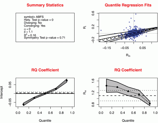
The upper-right panel of
Figure 1 shows an example for the stock Arkansas Best Corp (ticker ABFS). The Beta for Arkansas Best Corp using standard techniques would be about 1.1. Five different quantile regression lines are presented for
τ = 0.1, 0.3, 0.5, 0.7 and 0.9. The different portions of the individual returns that fall above and below the lines are apparent. Also shown, as a dotted line, is the OLS regression, which provides the traditional estimate of the Beta coefficient. In the lower-right panel, the black dots connected by the solid line represent the regression quantile estimates of the Beta coefficient
![Jrfm 07 00067 i002]()
for
τ = 0.1, 0.3, 0.5, 0.7 and 0.9. As we move from the left to the right with
τ increases from 0.1 to 0.9, we can see that the quantile regression estimates of Beta decrease from about
![Jrfm 07 00067 i005]()
= 1.44 to
![Jrfm 07 00067 i006]()
= 0.83 which reflects the declining slope of the quantile regression lines in the upper-right panel as we move from the lower quantile regression lines to the higher quantile regression lines. The grey band around the dots is the 95% confident band so that a particular
τ-th quantile regression Beta estimate
![Jrfm 07 00067 i002]()
is statistically different from 0 at a 5% level of significance when the band does not contain 0 for the chosen
τ. The horizontal dash line shows the value of the OLS estimated Beta
![Jrfm 07 00067 i007]()
with the horizontal dotted lines represent the 95% confidence band. The lower-left panel shows the regression quantile estimates of the alpha coefficient
![Jrfm 07 00067 i001]()
.
4. Heteroskedasticity
The presence of heteroskedasticity is apparent in
Figure 1 from the decreasing quantile regression Beta coefficients
![Jrfm 07 00067 i002]()
(decreasing risk) seen in the lower right graph as
τ increases (increasing returns
Rit or a gain frame). Also, the graph in the upper right corner shows that as the value of the market return
Rmt on the horizontal axis increases (a gain frame), the degree of variation of the individual return decreases (decreasing risk) and vice versa. These two features of this stock, Arkansas Best Corporation (ABFS), fulfill an investor’s preference for “loss-aversion” in a gain frame and “risk-seeking” in a loss frame as postulated by Kahneman and Tversky. We call this sort of heteroskedasticity a “converging heteroskedasticity” and is defined as a negative difference between the
τ = 0.9 and
τ = 0.1 Beta coefficients such that
![Jrfm 07 00067 i006]()
−
![Jrfm 07 00067 i005]()
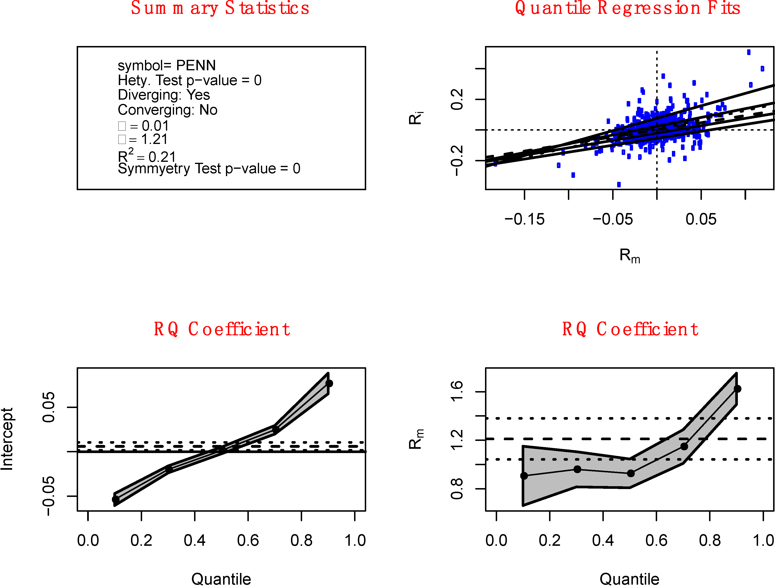
< 0 In contrast, the form of heteroskedasticity depicted in
Figure 2 is termed “diverging heteroskedasticity” and is defined as a positive difference between the
τ = 0.9 and
τ = 0.1 Beta coefficients such that
![Jrfm 07 00067 i006]()
−
![Jrfm 07 00067 i005]()
> 0. For this stock, Penn National Gaming (PENN), the lower right graph shows that the estimated Beta increases (increasing risk) for higher quantiles of
Rit (a gain frame). Also, the graph in the upper right shows that as the return on the market
Rmt increases (a gain frame), the variation of individual returns increases (increasing risk). This particular stock will be avoided by investors who are averse to loss in a gain frame and seek risk in a loss frame according to Kahneman and Tversky.
Figure 1.
Strong converging heteroskedasticity. The upper-left panel contains summary statistics of the chosen stock, which include the ticker symbol, p-value for the Wald test for heteroskedasticity, indicator for whether the stock is diverging, estimated Alpha and Beta, r-square, and the p-value for the test for symmetry of the stock return. The upper-right panel shows the various quantile regression fits of the Capital Asset Pricing Model (CAPM) model for τ = 0.1, 0.3, 0.5 (dash line), 0.7 and 0.9. The dotted line is the ordinary least squares (OLS) fit. The lower-left panel contains the quantile regression estimates of Alpha while the lower-right panel shows the quantile regression estimates of Beta for τ = 0.1, 0.3, 0.5, 0.7 and 0.9 along with their 95% confidence band. The dash line indicates the magnitude of the OLS Beta estimate while the dotted lines are the 95% confidence interval.
To test for the potential existence of diverging/converging heteroskedasticity in a particular stock, we can apply the Wald test for heteroskedasticity introduced by Koenker and Bassett [
12] and Koenker [
13] (p.76) to the following hypotheses:
H0:β0.9 − β0.1 = 0(no heteroskedasticity)
H0:β0.9 − β0.1 ≠ 0(diverging or converging heteroskedasticity)
When the null hypothesis is rejected by the Wald test at a chosen level of significance, there is an indication of the existence of diverging or converging heteroskedasticity. We can then determine the nature of heteroskedasticity by examining the sign of
![Jrfm 07 00067 i006]()
−
![Jrfm 07 00067 i005]()
.
We use the
rq function in the
quantreg package (Koenker [
14]) available from the GNU Free Software
R for statistical computing and graphics (R Development Core Team, [
15]) to compute the quantile regression coefficients in this study. The function uses a modified version of Barrodale and Roberts’s [
16] algorithm for L
1 regression as described in Koenker and d’Orey [
17,
18] for small sample sizes and the interior-point algorithm described in Koenker and Ng [
19] for large sample sizes. The standard error assumes local linearity of the conditional quantile functions and computes an Eicker-Huber-White sandwich estimate using a local estimate of the sparsity as described in Koenker [
13]. Koenker and Hallock [
20] is an excellent non-technical primer for quantile regression.
Figure 2.
Strong diverging heteroskedasticity. The upper-left panel contains summary statistics of the chosen stock, which include the ticker symbol, p-value for the Wald test for heteroskedasticity, indicator for whether the stock is diverging, estimated Alpha and Beta, r-square, and the p-value for the test for symmetry of the stock return. The upper-right panel shows the various quantile regression fits of the CAPM model for τ = 0.1, 0.3, 0.5 (dash line), 0.7 and 0.9. The dotted line is the OLS fit. The lower-left panel contains the quantile regression estimates of Alpha while the lower-right panel shows the quantile regression estimates of Beta for τ = 0.1, 0.3, 0.5, 0.7 and 0.9 along with their 95% confidence band. The dash line indicates the magnitude of the OLS Beta estimate while the dotted lines are the 95% confidence interval.
5. Interpretation of the Results
The sample of 4230 stocks is tested for the existence of converging or diverging heteroskedastictiy. The Wald test results are presented in
Table 1. We can see that 14.9% of the stocks (630 stocks) have
p-value smaller than 0.1. Hence, at the 10% level of significance, about 14.9% of the stocks exhibit either converging or diverging heteroskedasticity. By investigating the sign of
![Jrfm 07 00067 i006]()
−
![Jrfm 07 00067 i005]()
, we see that 10.6% (450 stocks) exhibit converging heteroskedasticity and will be preferred by investors with preference for “loss-aversion” in a gain frame and “risk-seeking” in a loss frame as postulated by Kahneman and Tversky while 4.3% (180 stocks) exhibit diverging heteroskedasticity and will be avoided.
Table 1.
Classification of heteroskedasticity. The table classifies the degree of converging and diverging heteroskedasticity into strongly, moderately, weakly and little or no heteroskedasticity. The smaller the p-value is for the Wald test for heteroskedasticity, the stronger is the degree of diverging or converging. Divergence or convergence is determined by the difference between the higher (β0.9) and lower regression quantiles (β0.1) for Beta. A negative difference with β0.9 − β0.1 < 0 is defined as converging while a positive difference β0.9 − β0.1 > 0 is called diverging. We propose that the 942 stocks that exhibit converging heteroskedasticity, in the top three lines of the chart, would be preferred to the 530 stocks that exhibit diverging heteroskedasticity in the bottom three lines of the chart.
| p value | Type of Heteroskedasticity | β0.9 − β0.1 | % of sample | Number of stocks |
|---|
| [0.0–0.1] | Strongly Converging | − | 10.6 | 450 |
| [0.1–0.2] | Moderately Converging | − | 6.6 | 280 |
| [0.2–0.3] | Weakly Converging | − | 5.0 | 212 |
| [0.3–1.0] | Little or no heteroskedasticity | − or + | 65.2 | 2758 |
| [0.2–0.3] | Weakly Diverging | + | 4.2 | 176 |
| [0.1–0.2] | Moderately Diverging | + | 4.1 | 174 |
| [0.0–0.1] | Strongly Diverging | + | 4.3 | 180 |
However, if one relaxes the level of significance in the Wald test to 20%, then a larger number of stocks, about 25.6% (1084 stocks) exhibit either converging or diverging heteroskedasticity. About 17.3% of these (730 stocks) exhibit converging heteroskedasticity while about 8.4% (354 stocks) exhibit diverging heteroskedasticity. So there is a continuum of the degree (strength) of diverging/converging heteroskedasticity. We can try to classify this using the value of
![Jrfm 07 00067 i006]()
−
![Jrfm 07 00067 i005]()
or the angle between
![Jrfm 07 00067 i006]()
and
![Jrfm 07 00067 i005]()
. The bigger the positive (negative) angle or the larger (smaller) the value of
![Jrfm 07 00067 i006]()
−
![Jrfm 07 00067 i005]()
, the stronger will be the degree of diverging (converging) heteroskedasticity. However, the angle between
![Jrfm 07 00067 i006]()
and
![Jrfm 07 00067 i005]()
as well as the value of
![Jrfm 07 00067 i006]()
−
![Jrfm 07 00067 i005]()
depends on the scatter of the individual return
Rit and the market return
Rmt. For two different stocks with the same angle between
![Jrfm 07 00067 i006]()
and
![Jrfm 07 00067 i005]()
or the same value in
![Jrfm 07 00067 i006]()
−
![Jrfm 07 00067 i005]()
, one of them can have a small
p-value that will render a rejection of the null hypothesis of no heteroskedasticity while the other can end up with a large
p-value that fails to reject the null hypothesis depending on the scatter of
Rit and
Rmt. Since the smaller the
p-value, the stronger is the evidence in the data against the null hypothesis of the absence of heteroskedasticity, we can try to classify the strength of heteroskedasticity using the delineation on the
p-value specified in
Table 1, where low
p-value indicates strong heteroskedasticity and high
p-value indicates little or no heteroskedasticity.
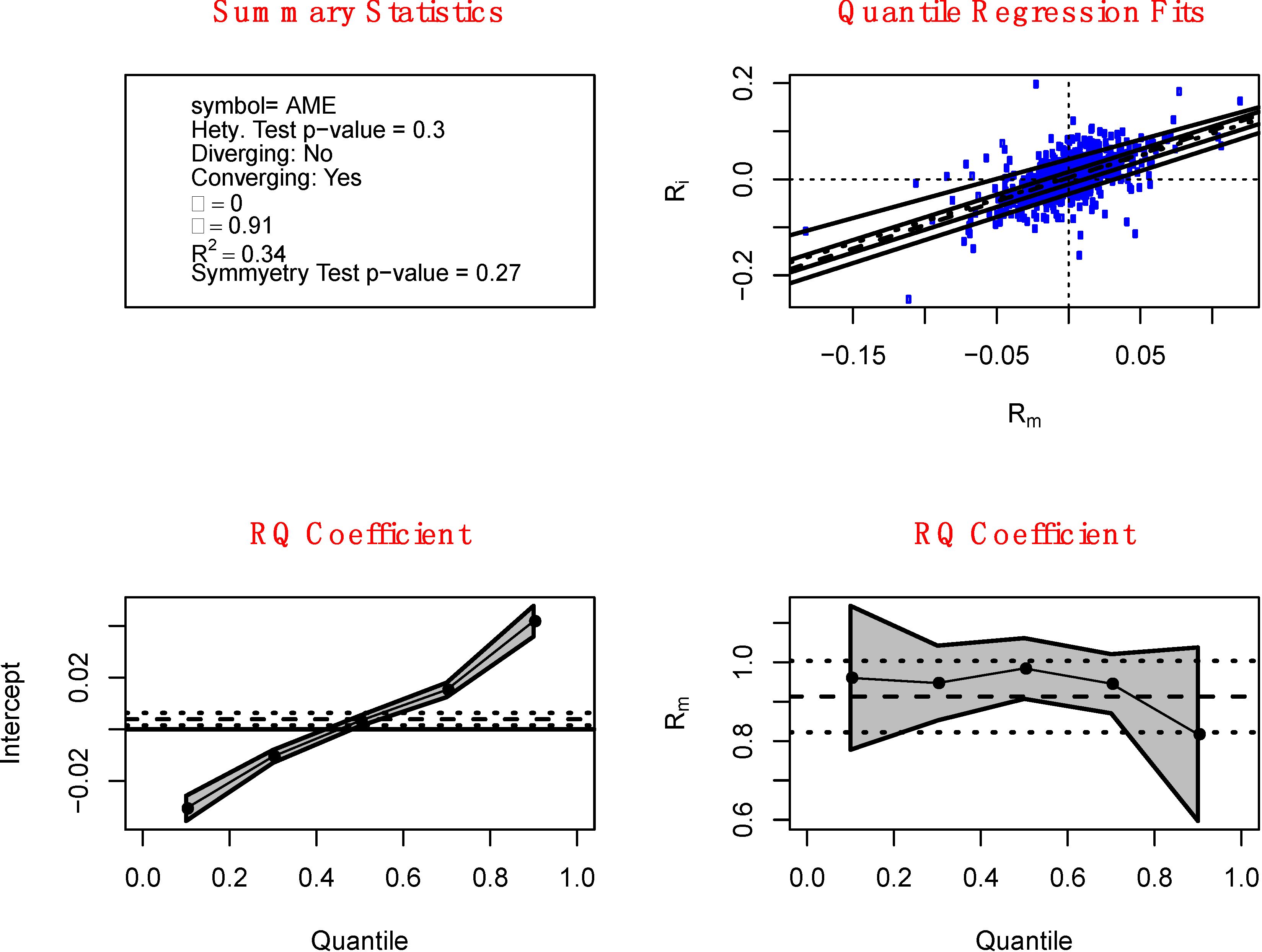
Figure 3 and
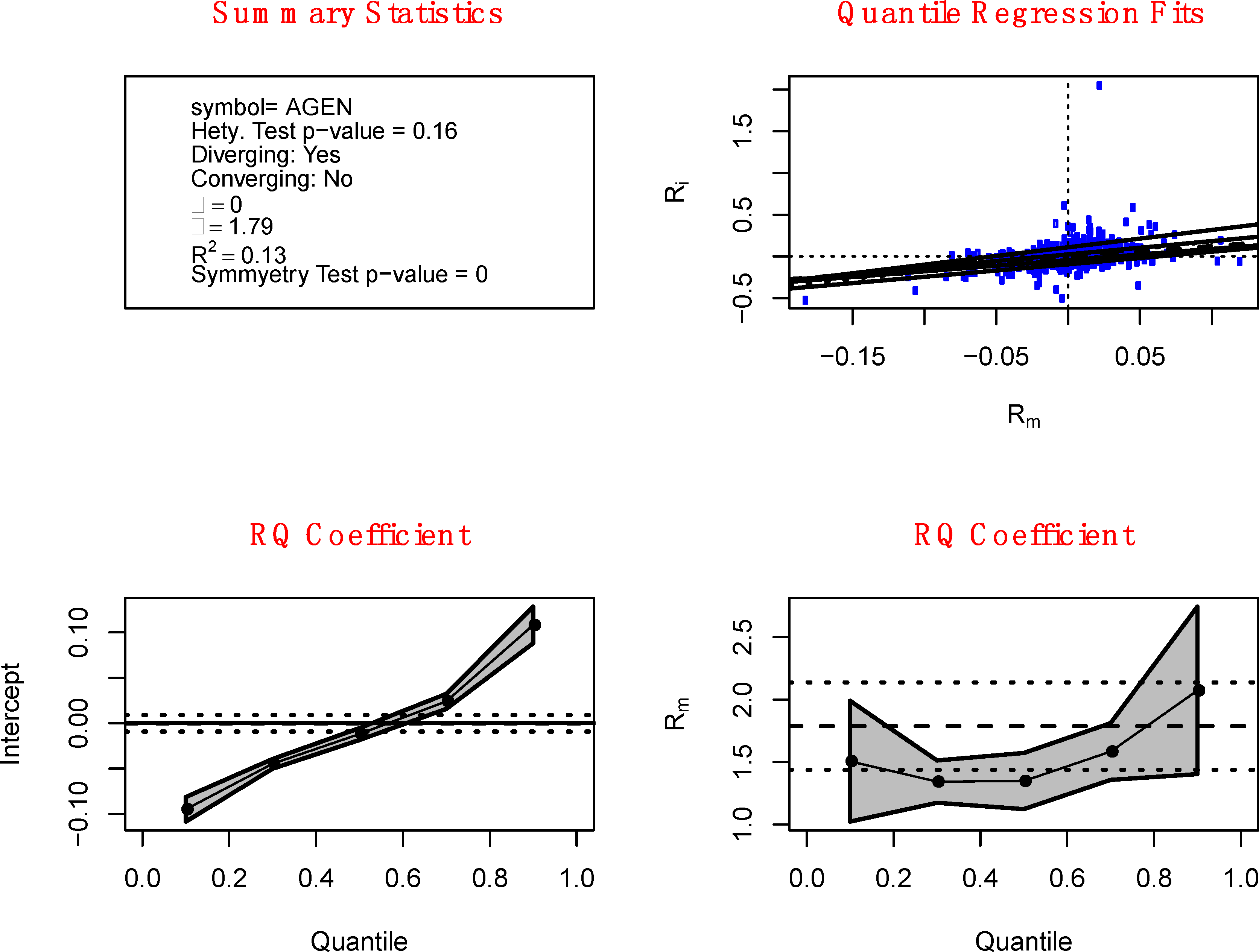
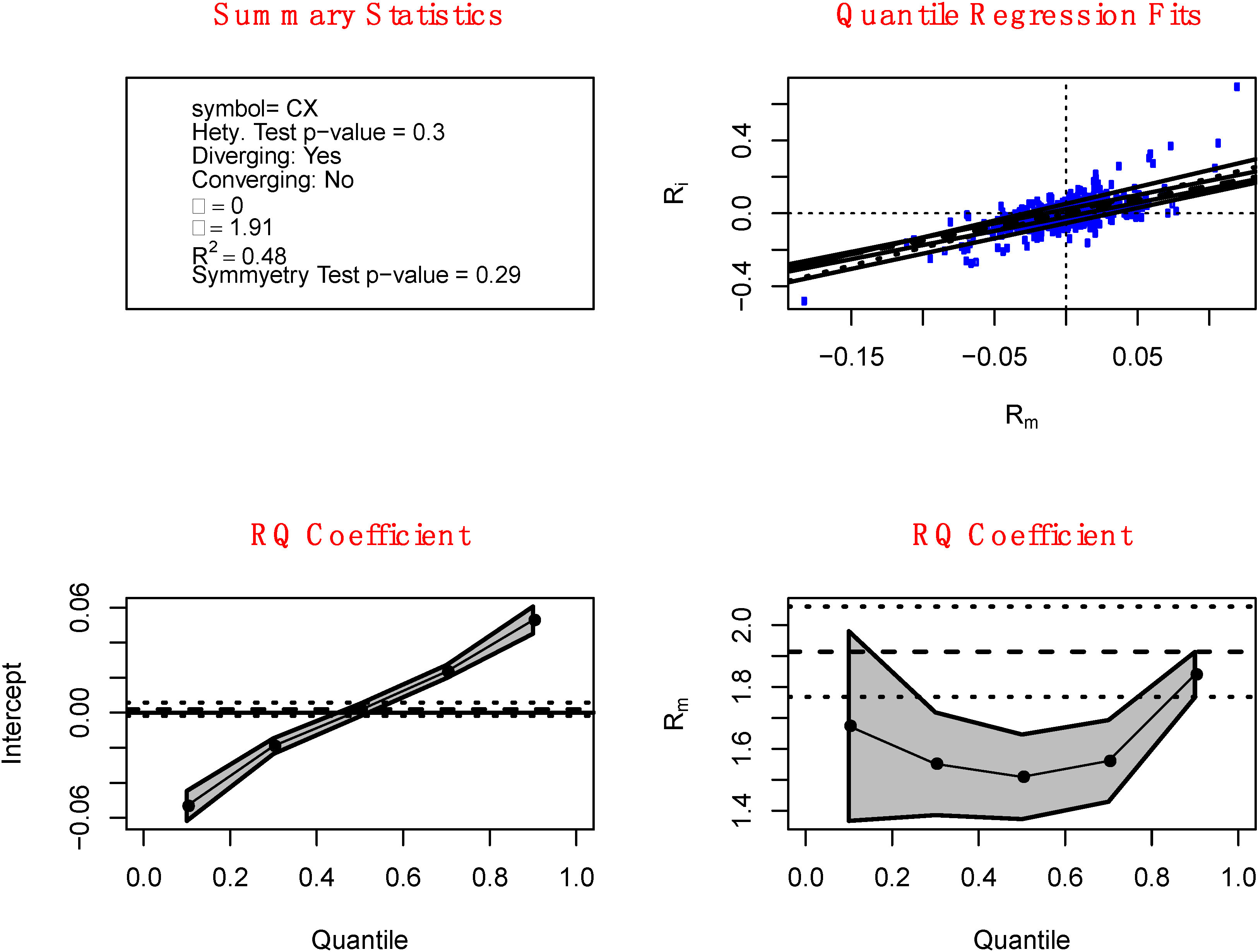
Figure 4 provide examples of sample stock returns with moderate and weak diverging heteroskedasticity, respectively. This is evident by the increasingly larger
p-values that can be found among the summary statistics in the upper left panel of the figures. Alternatively,
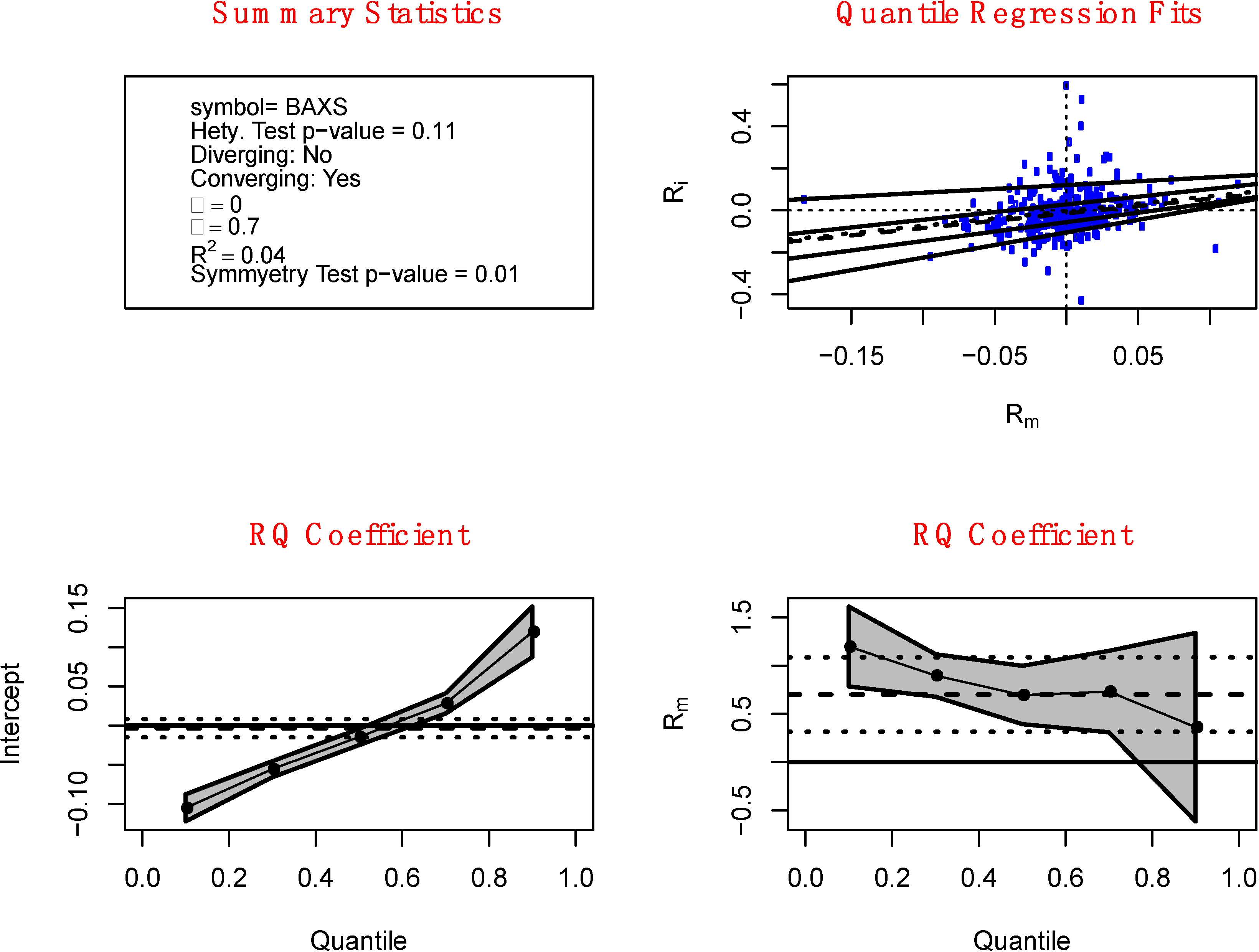
Figure 5 and
Figure 6 show examples of moderate and weak converging heteroskedasticity, respectively. As we move from
Figure 2 to
Figure 4, we can see from the upper left panels that the
p-value of the Wald test for heteroskedasticity increases from 0 to 0.16 and, eventually, to 0.3 as the degree of diverging heteroskedasticity diminishes. Likewise, as we move from
Figure 1 to
Figure 5 and
Figure 6, the
p-value increases from 0 to 0.11 and, eventually, to 0.3 as the degree of converging heteroskedasticity lessens. Also note that the Beta coefficient
![Jrfm 07 00067 i002]()
first falls as
τ increases from 0.1 to 0.3 and 0.5, and then rises as
τ increases to 0.7 and 0.9 in
Figure 4. The Wald test, however, is based on the difference between the two extreme Beta coefficients
![Jrfm 07 00067 i002]()
for
τ = 0.1 and 0.9. Therefore, as long as the positive difference
![Jrfm 07 00067 i006]()
−
![Jrfm 07 00067 i005]()
> 0 is significantly large, the test statistic will lead to the rejection of the null hypothesis of homoscedasticity and the conclusion of diverging heteroskedasticity.
Figure 3.
Moderate diverging heteroskedasticity. The upper-left panel contains summary statistics of the chosen stock, which include the ticker symbol, p-value for the Wald test for heteroskedasticity, indicator for whether the stock is diverging, estimated Alpha and Beta, r-square, and the p-value for the test for symmetry of the stock return. The upper-right panel shows the various quantile regression fits of the CAPM model for τ = 0.1, 0.3, 0.5 (dash line), 0.7 and 0.9. The dotted line is the OLS fit. The lower-left panel contains the quantile regression estimates of Alpha while the lower-right panel shows the quantile regression estimates of Beta for τ = 0.1, 0.3, 0.5, 0.7 and 0.9 along with their 95% confidence band. The dash line indicates the magnitude of the OLS Beta estimate while the dotted lines are the 95% confidence interval.
For the results in
Table 1, strong, moderate and weak heteroskedasticity are defined as having
p-values between 0.0–0.1, 0.1–0.2 and 0.2–0.3, respectively. For the sample of 4230 stocks, 10.6%, 6.6% and 5.0% showed strongly converging, moderately converging and weakly converging heteroskedasticity, respectively. In total, 22.2% of the sample (942 stocks) showed some degree of converging heteroskedasticity. Conversely, 4.3%, 4.1% and 4.2% showed strongly, moderately and weakly diverging heteroskedasticity. In total, 12.6% of the sample (530 stocks) showed some degree of diverging heteroskedasticity. The remaining 65.2% of the sample showed no significant heteroskedasticity.
Figure 4.
Weak diverging heteroskedasticity. The upper-left panel contains summary statistics of the chosen stock, which include the ticker symbol, p-value for the Wald test for heteroskedasticity, indicator for whether the stock is diverging, estimated Alpha and Beta, r-square, and the p-value for the test for symmetry of the stock return. The upper-right panel shows the various quantile regression fits of the CAPM model for τ = 0.1, 0.3, 0.5 (dash line), 0.7 and 0.9. The dotted line is the OLS fit. The lower-left panel contains the quantile regression estimates of Alpha while the lower-right panel shows the quantile regression estimates of Beta for τ = 0.1, 0.3, 0.5, 0.7 and 0.9 along with their 95% confidence band. The dash line indicates the magnitude of the OLS Beta estimate while the dotted lines are the 95% confidence interval.
One interpretation of these findings is that 22.2% of the stocks will fit the behavioral preference indicated by the Kahneman and Tversky [
3] findings. These stocks, showing converging heteroskedasticity, would be more preferred by investors than the other 77.8% of the stocks if all other factors are held constant. On the other side, 12.6% of the stocks show patterns that would not be optimum according to the Kahneman and Tversky [
3] findings. These stocks, showing diverging heteroskedasticity, would be less preferred by investors than the other 87.4% of the stocks, if all other factors are held constant.
Investors are always looking for any possible indicator that can help them improve their portfolios. Even small improvements can provide benefits to investors’ utility. The results presented may give new information about 34.8% of the universe of stocks that investors choose from. When a portfolio can be chosen that more aligns with investors preferences, it may be a benefit to investors.
Figure 5.
Moderate converging heteroskedasticity. The upper-left panel contains summary statistics of the chosen stock, which include the ticker symbol, p-value for the Wald test for heteroskedasticity, indicator for whether the stock is diverging, estimated Alpha and Beta, r-square, and the p-value for the test for symmetry of the stock return. The upper-right panel shows the various quantile regression fits of the CAPM model for τ = 0.1, 0.3, 0.5 (dash line), 0.7 and 0.9. The dotted line is the OLS fit. The lower-left panel contains the quantile regression estimates of Alpha while the lower-right panel shows the quantile regression estimates of Beta for τ = 0.1, 0.3, 0.5, 0.7 and 0.9 along with their 95% confidence band. The dash line indicates the magnitude of the OLS Beta estimate while the dotted lines are the 95% confidence interval.
Investors could measure the type and degree of heteroskedasticity for individual stocks. Those that exhibit converging heteroskedasticity should be preferred over other stocks. Those stocks that exhibit diverging heteroskedasticity would not be preferred over other stocks.
We should emphasize that the decision of defining strong, moderate and weak heteroskedasticity based on
p-value between 0.0–0.1, 0.1–0.2 and 0.2–0.3, respectively, is somewhat arbitrary. One can always argue for other delineations of the
p-value for the three classifications of strong, moderate and weak heteroskedasticity. Likewise, the choice of measuring the diverging/converging heteroskedasticity based on the interdecile range
![Jrfm 07 00067 i006]()
−
![Jrfm 07 00067 i005]()
is also somewhat arbitrary. One can also argue for the use of the difference between other pairs of the estimated Beta, e.g., the interquartile range
![Jrfm 07 00067 i008]()
−
![Jrfm 07 00067 i009]()
, to define diverging/converging heteroskedasticity. At the journal’s website, we provide an
R function
beta-het that is used to generate
Figure 1 through
Figure 6 and compute the various summary statistics reported in the upper-left panel of those figures. Investors could use the function to experiment with different possible delineations of the
p-value and the different pairs of estimated Betas. This could help them define and quantify the strength of diverging/converging heteroskedasticity to suit their different degrees of preference for “loss-aversion” in a gain frame and “risk-seeking” in a loss frame.
Figure 6.
Weak converging heteroskedasticity. The upper-left panel contains summary statistics of the chosen stock, which include the ticker symbol, p-value for the Wald test for heteroskedasticity, indicator for whether the stock is diverging, estimated Alpha and Beta, r-square, and the p-value for the test for symmetry of the stock return. The upper-right panel shows the various quantile regression fits of the CAPM model for τ = 0.1, 0.3, 0.5 (dash line), 0.7 and 0.9. The dotted line is the OLS fit. The lower-left panel contains the quantile regression estimates of Alpha while the lower-right panel shows the quantile regression estimates of Beta for τ = 0.1, 0.3, 0.5, 0.7 and 0.9 along with their 95% confidence band. The dash line indicates the magnitude of the OLS Beta estimate while the dotted lines are the 95% confidence interval.

 and
and  , minimize the following objective function:
 τ|Rit −
  (1 − τ)|Rit −
  = 1.44 to
  = 0.83 which reflects the declining slope of the quantile regression lines in the upper-right panel as we move from the lower quantile regression lines to the higher quantile regression lines. The grey band around the dots is the 95% confident band so that a particular τ-th quantile regression Beta estimate
  with the horizontal dotted lines represent the 95% confidence band. The lower-left panel shows the regression quantile estimates of the alpha coefficient
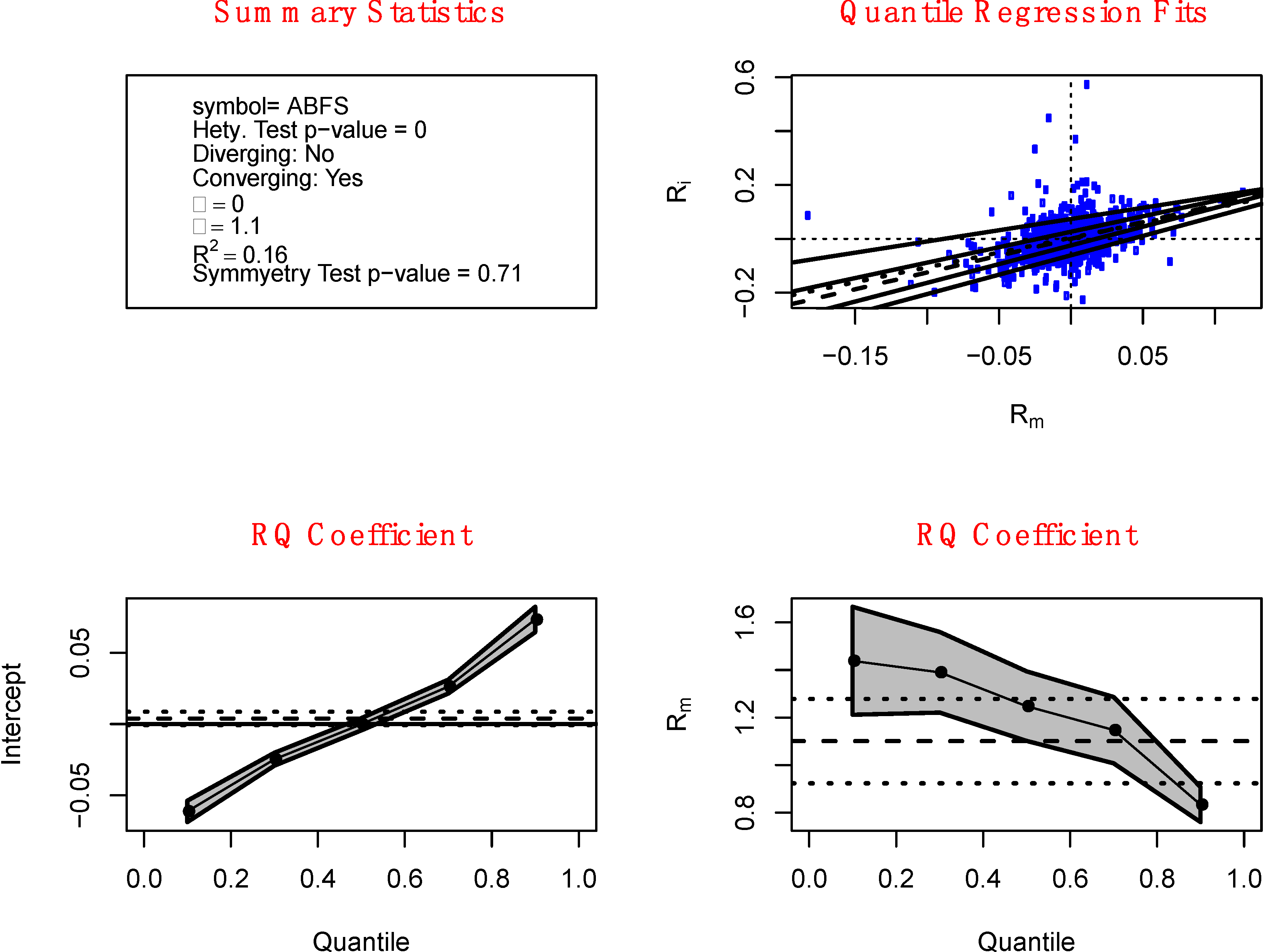

 −
−  , to define diverging/converging heteroskedasticity. At the journal’s website, we provide an R function beta-het that is used to generate Figure 1 through Figure 6 and compute the various summary statistics reported in the upper-left panel of those figures. Investors could use the function to experiment with different possible delineations of the p-value and the different pairs of estimated Betas. This could help them define and quantify the strength of diverging/converging heteroskedasticity to suit their different degrees of preference for “loss-aversion” in a gain frame and “risk-seeking” in a loss frame.