Models for Risk Aggregation and Sensitivity Analysis: An Application to Bank Economic Capital

Abstract

A challenge in enterprise risk measurement for diversified financial institutions is developing a coherent approach to aggregating different risk types.  This has been motivated by rapid financial innovation, developments in supervisory standards (Basel 2) and recent financial turmoil.  The main risks faced - market, credit and operational – have distinct distributional properties, and historically have been modeled in differing frameworks.   We contribute to the modeling effort by providing tools and insights to practitioners and regulators.  First, we extend the scope of the analysis to liquidity and interest rate risk, having Basel Pillar II of Basel implications.  Second, we utilize data from major banking institutions’ loss experience from supervisory call reports, which allows us to explore the impact of business mix and inter-risk correlations on total risk.  Third, we estimate and compare alternative established frameworks for risk aggregation (including copula models) on the same data-sets across banks, comparing absolute total risk measures (Value-at-Risk – VaR and proportional diversification benefits-PDB), goodness-of-fit (GOF) of the model as data as well as the variability of the VaR estimate with respect to sampling error in parameter.  This benchmarking and sensitivity analysis suggests that practitioners consider implementing a simple non-parametric methodology (empirical copula simulation- ECS) in order to quantify integrated risk, in that it is found to be more conservatism and stable than the other models.  We observe that ECS produces 20% to 30% higher VaR relative to the standard Gaussian copula simulation (GCS), while the variance-covariance approximation (VCA) is much lower.  ECS yields the highest PDBs than other methodologies (127% to 243%), while Archimadean Gumbel copula simulation (AGCS) is the lowest (10-21%).  Across the five largest banks we fail to find the effect of business mix to exert a directionally consistent impact on total integrated diversification benefits.  In the GOF tests, we find mixed results, that in many cases most of the copula methods exhibit poor fit to the data relative to the ECS, with the Archimadean copulas fitting worse than the Gaussian or Student-T copulas.  In a bootstrapping experiment, we find the variability of the VaR to be significantly lowest (highest) for the ECS (VCA), and that the contribution of the sampling error in the parameters of the marginal distributions to be an order or magnitude greater than that of the correlation matrices.

INTRODUCTION AND SUMMARY

A modern diversified financial institution, engaging in a broad set of activities (e.g., banking, brokerage, insurance or wealth management) is faced with the task of measuring and managing risk across all of these. It is the case that just about any large, internationally active financial institution is involved in at least two of these activities, and many of these are a conglomeration of entities under common control. Therefore, we have the necessity of a framework in which disparate risk types can be aggregated. However, this is challenging, due to the varied distributional properties of the risks1. It is accepted that regardless of which sectors a financial institution focuses upon, they at least manage credit, market and operational risk. The corresponding supervisory developments - the Market Risk Amendment to Basel 1, Advanced IRB to credit risk under Basel 2 and the AMA approach for operational risk (BCBS 1988, 1996, 2004) – have given added impetus for almost all major financial institutions to quantify these risks in a coherent way.

Furthermore, regulation is evolving toward even more comprehensive standards, such as the Basel Pillar II Internal Capital Adequacy Assessment Process (ICAAP) (BCBS, 2009). In light of this, institutions may have to quantify and integrate other risk types into their capital processes, such as liquidity, funding or interest income risk. A quantitative component of such an ICAAP may be a risk aggregation framework to estimate economic capital (EC)2. A key contribution of our paper is providing analytical techniques around several activities that are supervisory expectations in the context of ICAAP for institutions having EC models. First, we employ sensitivity analysis3, and accuracy testing of the EC model, in both cases assessing the likely ranges of the EC model quantile estimates. These two are accomplished through quantifying the variability in EC risk measures resulting from sampling error in the estimation of key parameters (estimation of marginal distributions and correlations). We also conduct benchmarking of models4, a type of validation exercise for an EC framework, by comparing EC risk measures across different frameworks for aggregating risks (or copula model) for a given bank, as well as across banks for a given modeling framework.

The central technical and conceptual challenge to risk aggregation lies in the diversity of distributional properties across risk types. In the case of market risk, a long literature in financial risk management has demonstrated that portfolio value distributions may be adequately approximated in a Gaussian, due to the symmetry and thin tails that tend to hold at an aggregate level in spite of non-normalities at the asset return level (Jorion, 2006).5 In contrast, credit loss distributions are characterized by pronounced asymmetric and long-tailed distributions, a consequence of phenomena such as lending concentrations or credit contagion, giving rise to infrequent and very large losses. This feature is magnified for operational losses, where the challenge is to model rare and severe losses due to exogenous events, such failures of systems or processes, litigation or fraud (e.g., the Enron or Worldcom debacles, or more recently Societe Generale).6 While the literature abounds with examples of these three (Crouhy et al., 2001), little attention has been paid to the even broader range of risks faced by a large financial institution (Kuritzkes et al., 2003), including liquidity and asset / liability mismatch risk.

Certain risk types are more amenable to estimation, such as market risk, while others present a greater challenge, such as operational risk. In the case of the former, there is richer data available and well established methodologies, in order to estimate distributions. Unfortunately, for the latter we deal with a paucity of data, and the techniques available for fitting such distributions are just recently being developed. Furthermore, little is known about how these risk types relate to one another. In order to address this, we build upon the method of copulas, an approach that has become popular within the operational risk realm itself, stemming from the necessity of having to combine a large number of risk types. This methodology combines separate marginal distributions in a coherent and plausible manner, preserving key distributional features such as skewness and excess kurtosis. Furthermore, this technique has the advantage of handling situations in which little is known about relationships amongst random variables, requiring only some measure of codependence (such as correlation). We compare various copula models, as well as other methods for the construction of a joint distribution of losses, such as simple addition or the correlation matrix approach.7

The empirical exercise uses regulatory call report data to proxy for the losses from the various risk types. The empirical analysis focuses upon five of the largest financial conglomerates (JP Morgan Chase, Citigroup, Wells Fargo, Wachovia and Bank of America), available on a quarterly frequency, commencing in the 1^st quarter of 1984. The rationale for concentrating on large banks is motivated in large part by the intense policy debate surrounding the New Basel Capital Accord (BCBS, 2004). The most recent incarnation of Basel incorporates operational risk, a new risk type to the regulatory calculation, which differs substantially in distributional characteristics from market and credit risk. The importance of this is highlighted by the conclusions of the BCBS Joint Forum (2001, 2003), which highlights quite clearly how banks and insurers are actively wrestling with this. While the focus herein is upon the banking sector, our methodology could just as easily extend any other kind of financial conglomerate such as an insurer.

This study is part of a burgeoning literature that performs a comprehensive analysis around how to combine a set of underlying risk factors influencing the total risk of large financial institutions. Furthermore, our work is among first to utilize publicly available, industry-wide data to perform to this end8. In particular, we are able to study enterprise-wide risk across alternative risk aggregation measures (or dependence structures) and across institutions. We analyze actual data from a set of large financial institutions, in contrast with many of the previous studies that have used simulated data to model risk distributions. Furthermore, as these institutions have varying business mixes, we are able to examine the sensitivity of risk estimates to this. Such analysis is relatively rare in the literature, and even among the studies conducting such, this has generally involved either a rather limited set of risk factors, or has been limited to the loss experience of a single institution, which creates challenges for generalizing the results. A notable exception to this trend in the literature is Rosenberg and Schuermann (2006), who analyze a panel of quarterly data for a set of large banks, developing empirical proxies for different risk types (credit, market and operational), and employ the method of copulas to aggregate these. We follow a similar empirical strategy, utilizing the same type of data extracted from regulatory filings, giving us confidence that results obtained are representative of a typical institution. We propose to extend this framework in several ways. First, we consider a wider range of risk types. Second, we investigate both the magnitudes of risk measures and the goodness-of-fit to the data of alternative risk aggregation methodologies. Finally, we perform sensitivity analysis by studying the variability of different risk measures that is a consequence of sampling error, through a bootstrap experiment.

Our main results are as follows. Through differences observed across the five largest banks by book value of assets as of 4Q089, we find in regard to different risk aggregation methodologies significant variation amongst absolute measures of risk. Dollar 99.97^th percentile Value-at-Risk (VaR) is increasing in size of institution, but expressed as a proportion of book value it appears to be decreasing in size of the entity. Across different risk aggregation methodologies and banks we observe that the empirical copula simulation (ECS) and Archimadean-Gumbel copula simulations (AGCS) to produce the highest absolute magnitudes of VaR as compared to the Gaussian copula simulation (GCS), Student-T copula simulation (STCS) or any of the other Archimadean copulas. The variance-covariance approximation (VCA) produces the lowest VaR. The proportional diversification benefits, as measured by the relative VaR reduction vis a vis the assumption of perfect correlation, exhibit radical variation across banks and aggregation techniques. The ECS generally yields the highest values than the other methodologies (127% to 243%), the GCS “benchmark” (41-58%) and VCA (31-40%) toward the middle to lower end of the range, while the AGCS is the lowest (10-21%). We conclude that while ECS (VCA) may over-state (under-state) absolute (relative) risk, on the order of about 20% to 30% across all banks, proportional diversification benefits are generally understated (overstated) by the VCA (ECS) relative to standard copula formulations on the order of about 15% to 30% (3 to 6) across all banks and frameworks, respectively. Through differences observed across the five largest banks, we fail to find business mix10 to exert a directionally consistent an impact on total integrated risk or proportional diversification benefits above and beyond exposure to, and correlation amongst, underlying risk factors. In an application of the goodness-of-fit tests for copula models, developed by Genest et al (2009), we find mixed results and in many cases that commonly utilized parametric copula models fail to fit the data. In a bootstrapping experiment, we are able to measure the variability in the VaR integrated risk and proportional diversification benefit measures, which can be interpreted as a sensitivity analysis (Gourieroux et al, 2000.) In this experiment we find the variability of the VaR to be significantly lower for the EC, and significantly greater for the VCA, as compared to other standard copula formulations. However, amongst copula models we find that the contribution of the sampling error in the parameters of the marginal distributions to be an order or magnitude greater than that of the correlations. Taken as a whole, our results constitute a sensitivity analysis that argues for practitioners to err on the side of conservatism in considering a non-parametric copula alternative in order to quantify integrated risk.

The remainder of the paper is organized as follows. Section 2 presents a brief overview of the related literature. Section 3 follows with a discussion of various risk aggregation frameworks. Section 4 presents the data analysis: descriptive statistics and the marginal risk distributions by risk type. In Section 5, we present our analytical results by examining the impact of alternative aggregation methodologies on the integrated risk measure across banks, both in absolute terms and also its variability. Section 6 provides final comments and directions for future research.

1.  REVIEW OF THE LITERATURE

Risk management as a discipline in its own right, distinct from either general finance or financial institutions, is a relatively recent phenomenon. It follows that the risk aggregation question has only recently come into focus. To this end, the method of copulas, which follows from a general result of mathematical statistics due to Sklar (1956), readily found an application. This technique allows the combination of arbitrary marginal risk distributions into a joint distribution, while preserving a non-normal correlation structure. Among the early academics to introduce this methodology is Embrechts et al. (1999, 2002). This was applied to credit risk management and credit derivatives by Li (2000). The notion of copulas as a generalization of dependence according to linear correlations is used as a motivation for applying the technique to understanding tail events in Frey and McNeil (2001). This treatment of tail dependence contrasts to Poon et al (2004), who instead use a data intensive multivariate extension of extreme value theory, which requires observations of joint tail events.

Most of the applications of copula theory seen in finance have been in the domain of portfolio risk measurement, examples including Bouye (2001), Longin and Solnik (2001) and Glasserman et al (2002)11. In a notable paper, Embrechts et al. (2003) reviews and extends some of the more recent results for finding distributional bounds for functions of dependent risks, with the main emphasis on Value-at-Risk as a risk measure. On the other hand, it is rare to find papers in the financial institutions area, where the application would be for risk aggregation. The joint distribution of market and credit risk in a banking context is analyzed by Alexander and Pezier (2003), who instead of a copula use a common risk factor model. In the setting of an insurance company, Wang (1998) lays a theoretical framework and surveys various modeling approaches to enterprise-wide risk, in the setting of heterogeneous risk types. In the case of a diversified insurer with both property & casualty and life insurance business segments, Ward and Lee (2002) model the joint loss distribution using pair-wise roll-ups with a Gaussian copula 12. Notable here is that marginal distributions are computed both analytically as well as numerically, for example in the cases of credit (a beta distribution) and life insurance / mortality (Monte Carlo simulation), respectively. Furthermore, a rather broad set of risks are analyzed relative to the previous literature, in this case non-catastrophe liability, catastrophe, mortality, asset-liability mismatch (ALM), credit, market and operational risk. In another study, similar to Ward and Lee (2002) in that risks are modeled in a pairwise fashion, Aas and Dimakos (2004) estimate the joint loss distribution in the setting of a bank having a life insurance subsidiary. In this model, total risk is sum of the conditional marginal risk and unconditional credit risk, which is achieved by imposing conditional independence through a set of sufficient conditions, such that only pair-wise dependence remains. Simulation experiments indicate that while total risk measured using “near tails” (i.e., 95–99%) is only about 10% less than addition of individual risks, using “far” tail (i.e., 99.97%) is about 20% less, suggestive of the importance of diversification effects for accurate risk aggregation in the tails.

Kuritzkes et al. (2003), in the setting of a financial conglomerate and in a Gaussian copula framework having analytic solutions, arrive at a large set of diversification results by through varying a range of input parameters. Similarly to Dimakos and Aas (2004), addition of individual risks is found to overstate total diversified risk, although the differences are less than the former study (about 15% across market, credit, and operational risk for a bank; 20–25% for insurers; and 5–15% for a “bank-assurance” style financial conglomerate.)

In are recent study, Schuermann and Rosenberg (2006) study integrated risk management for typical large, internationally active financial institution. They develop an approach for aggregating three main risk types (market, credit, and operational) where the distributional properties amongst them varies widely. The authors build the distribution of total risk using the method of copulas, which allows them to incorporate realistic features of the marginal distributions (e.g., well documented empirical skewness and leptokurtosis of financial returns and credit losses), while at the same time preserving a flexible dependence structure. Exploring the impact of business mix and inter-risk correlation on total risk, the former are found to be more important than the latter, which is interpreted as “good news” for financial supervisors. They also compare the copula methodology with various approaches simplified applied by practitioners, such as the variance-covariance and the simple addition approaches, thereby documenting how the latter may overstate total risk.

Aas et al (2007) present a new approach to determining the risk of a financial institution, including components for the standard risk types (credit, market, operational and business), and additional ownership risk faced in the context of owning a life insurance subsidiary. Due to lack of appropriate data for certain risk types, this model combines a base-level with top-level aggregation mechanisms. Economic risk factors used in the bottom-up component are described by a multivariate GARCH model with Student-t distributed errors, and the loss distributions for different risk types determined by non-linear functions of these factors. This implies that these marginal loss distributions are correlated indirectly through the relationship between risk factors. The model, originally developed DnB Nor (the largest financial institution in Norway), is adapted to the requirements of Basel II.

Aas and Berg (2007) review models for construction of higher-dimensional dependence that have arisen recent years. The authors argue that in a multivariate data-set, which exhibits complex patterns of dependence (particularly in the tails), risk can be modeled using a cascade of lower-dimensional copulae. They examine two such models that differ in their construction of the dependency structure, the nested Archimedean and the pair-copula constructions (also referred to as “vines”). The constructions are compared, and estimation and simulation techniques are examined. The fit of the two constructions is tested on two different four-dimensional data sets, precipitation values and equity returns, using a state of the art copula goodness-of-fit procedure. The nested Archimedean construction is strongly rejected for both data-sets, while the pair-copula construction provides an appropriate fit. Through VaR calculations, they show that the latter does not over-fit data, but works very well even out-of-sample.

Several proposals have been made recently of goodness-of-fit tests for copula models. Genest et al (2009) briefly and critically review this literature and propose a “blanket test”, which requires neither arbitrary categorization of the data, nor “strategic” choices of non-parametric settings such as smoothing parameters, weight functions, kernels, windows, etc. The null distribution is the empirical copula and does not depend upon the choice of marginal distributions. They describe the results of a large-scale Monte Carlo experiment designed to assess the effect of sample size and strength of dependence on the level and power of the blanket tests for various combinations of copula models under the null hypothesis and the alternative. In order to circumvent problems in the determination of the limiting distribution of the test statistics under composite null hypotheses, they recommend the use of a double parametric bootstrap procedure, whose implementation is detailed and practical recommendations rendered.

2.  ESTIMATION METHODOLOGY: ALTERNATIVE RISK AGGREGATION FRAMEWORKS

The concept of risk is conventionally framed in terms of a divergence between an expected outcome and an adverse result with respect to some phenomenon of interest. Depending upon the application or risk type, these quantities may include valuations, cash flows, levels of loss or the severities associated with an event of default. Conventionally, this profile has been characterized by a mathematical object known as a probability distribution, which quantifies potential outcomes and their associated relative likelihoods of occurrence13. Risk can, and has commonly been, described by the some measure of the entropy or dispersion of a probability distribution such as a standard deviation (or variance).14 However, unless one is dealing with a normal or Gaussian distribution 15, this measure is not sufficient to characterize risk as we conceptualize it both in economics as well as herein. Once we depart from normality, then simple measures of dispersion such as the standard deviation fail to provide a complete description of risk as we understand it. There may exist arbitrarily many distributions having the same such measure but also having very different shapes, such that risk could vary dramatically. When particularly concerned with adverse outcomes and the tails of the distribution, directly connected to the concept of downside risk, we may find these to be divergent for distributions having the same standard deviation. In that case, one must attempt to quantify higher moments of the probability distribution, such as skewness or kurtosis. A popular way to cope with non-normality, which has been long documented as a feature of asset prices (Mandelbrot, 1963) and more recently for varied risk types, is to analyze a quantile of a distribution as in a “Value-at-Risk” measure (VaR). This is usually framed in a statement that we can, with a certain probability (or percent of the time), expect some risk factor of interest to not exceed an extreme value. Such an approach, while subject to severe criticism from a theoretical perspective regarding it as not being a “coherent” measure of risk (Artzner et al, 1997, 1999), has nevertheless become standard in the industry16. Setting aside this debate for now, we will briefly describe the VaR, or what we prefer to term the “risk quantile approach” (RQA) to quantifying adverse financial or economic outcomes.

2.1  Value-at-Risk (VaR)

VaR is one of the industry standard approaches for measuring risk due to adverse outcomes. A basic description of this risk measure is as a high quantile of a loss distribution, whereby convention levels of risk are defined as higher realizations of a vector of risk factors; if the context involves profit and loss (“P&L”), then it is understood that we are taking the negative of the dollar amounts, so that higher values indicate losses. Let us denote a vector of K risk factors at time t by $X_t=\left(X_{1t},\mathrm{..},X_{Kt}\right)$, having joint distribution function $F_X\left(X\right)\equiv \mathrm{Pr}\left(X_1\le x_1,\mathrm{..},X_K\le x_K\right)$. Let us consider a single-valued function of the risk factors $\text{Π}:R^K\to R$, which could be the aggregate losses on a set of dollar positions from time t to time t + Δ (where Δ is the horizon 17), such as the simple sum of losses ${\text{Π}}_{t,t+\text{Δ}}\left(X_t\right)={\displaystyle \sum _{i=1}^k{X}_{t,i}}$ that we consider herein. The VaR at the α^th confidence level between times t and t + Δ, denoted as $Va{R}_{t,t+\text{Δ}}^{\text{Δ}\left(X\right)}\left(\alpha \right)$, is related to the α^th quantile of $F_{\text{Π}\left(X\right)}\left(\text{Π}\left(X\right)\right)$ by18:

$$\mathrm{Pr}\left(\text{Π}\left(X_{t+\text{Δ}}\right)\ge Va{R}_{t,t+\text{Δ}}^{\text{Π}\left(X\right)}\left(\alpha \right)\right)=1-F_{\text{Π}\left(X\right)}\left(Va{R}_{t,t+\text{Δ}}^{\text{Π}\left(X\right)}\left(\alpha \right)\right)=1-\alpha$$

(1)

This implies that the VaR is given by19:

$$Va{R}_{t,t+\text{Δ}}^{\text{Π}\left(X\right)}\left(\alpha \right)=F_{\text{Π}\left(X\right)}^{-1}\left(\alpha \right)$$

(2)

VaR is meant to provide a compact summary measure of the risk with respect to a set of factors, analogously to the concept of a sufficient statistic that characterizes the distribution of a random variable. While there are many compelling arguments that this analogy is strained, and that in managing and measuring risk one should focus on the entire distribution rather than a summary measure (Diebold et al, 1998; Christoffersen and Diebold, 2000; Berkowitz, 2001), nevertheless interest in a simpler summary measure continues. Artzner et al. (1997, 1999) lay out a set of criteria necessary for what they term a ‘‘coherent’’ measure of risk. The first such criterion is homogeneity, which is the requirement that risk be increasing in the size of positions. Second, monotonicity, is the notion that we consider a portfolio having systematically lower returns than another, for all states of the world, to have greater risk. Subadditivity is the condition that the risk of a collection of positions (such as a weighted average or a simple sum) cannot be greater than the collection of such risks. Finally, the risk-free condition stipulates that as the proportion of a portfolio invested in the risk-free asset increases, the risk of the portfolio risk should not be increasing. It is well-known that unless the underlying risk factors come from the family of elliptical distributions, which subsumes the Gaussian, then VaR does not satisfy subadditivity. The implication of this is that in such a situation it is possible to take concentrated positions in one exposure in such a way that the risk of that exposure is just shy the overall portfolio VaR threshold (Embrechts et al. 1999, 2002). A risk metric closely related to VaR, which is coherent, is the expected shortfall (ES). This measures the expectation of the risk exposure conditional upon exceeding a VaR threshold:

$$E{S}_{t,t+\text{Δ}}^{\text{Π}\left(X\right)}\left(\alpha \right)={\mathrm{E}}_t\left[\text{Π}\left(X_{t+\text{Δ}}\right)|\text{Π}\left(X_{t+\text{Δ}}\right)>Va{R}_{t,t+\text{Δ}}^{\text{Π}\left(X\right)}\left(\alpha \right)\right]$$

(3)

The issue that arises with the ES risk measure is the choice of the VaR cutoff. We will report ES results corresponding to a conventional confidence level of 0.99, which yields magnitudes close to the conventional level of 0.9997 for economic or regulatory capital.

An interesting and ubiquitous special case that we consider here, motivated by the mean-variance investment theory of Markowitz (1959) and seen in many economic capital frameworks amongst banking practitioners, is where risk factors have a valid variance-covariance matrix and either risk factors are multivariate Gaussian, or risk managers and investors do not care about moments higher than the 2^nd 20:

$${\Sigma }_{t+\text{Δ}}={\mathrm{V}}_t\left[X_{t+\text{Δ}}\right]=E_t\left[{\left(X_{t+\text{Δ}}-E_t\left[X_{t+\text{Δ}}\right]\right)}^T\left(X_{t+\text{Δ}}-E_t\left[X_{t+\text{Δ}}\right]\right)\right]$$

(4)

Where ${\mathrm{V}}_t\left[X_{t+\text{Δ}}\right]$ is the time t variance of vector $X_{t+\text{Δ}}$. Note that we are assuming the risk factors to be dollar exposures, so that we do not have the portfolio weights of the familiar expression for portfolio variance. That is, our total time t risk exposure at ${\text{Π}}_{t,t+\text{Δ}}$ is simply the sum of the constituent risks:

$${\text{Π}}_{t,t+\text{Δ}}=i_K^T{X}_{t,i}={\displaystyle \sum _{i=1}^K{X}_{t,i}}$$

(5)

It follows from (3.1.4) and (3.1.5) that the standard deviation of the position is given by the square-root of quadratic form:

$$S_t\left[{\text{Π}}_{t,t+\text{Δ}}\right]=\sqrt{{i_k}^T{\Sigma }_{t,t+\text{Δ}}{i}_k}=\sqrt{{\displaystyle \sum _{i=1}^K{\sigma }_{t,i}^2+2}{\displaystyle \sum _{i\ne j}^K{\rho }_{t,ij}{\sigma }_{t,i}{\sigma }_{t,j}}}$$

(6)

Where $Va{r}_t\left(X_{t,i}\right)={\sigma }_{t,i}^2$ and ${\rho }_{t,ij}=\frac{Co{v}_t(X_{t,i},X_{t,j})}{\sqrt{Va{r}_t\left(X_{t,i}\right)Va{r}_t\left(X_{t,j}\right)}}$ are the univariate variance and linear (Pearson) correlation coefficients, respectively. Note that we retain the time subscript in the 2^nd moments to remind ourselves of the dynamic nature of this problem in a general context. To illustrate, suppose that we have 3 risk factors $X_t=\left(X_{1t},X_{2t},X_{3t}\right)$ 21. In this case we get the familiar expression:

$$S_t\left[{\displaystyle \sum _{i=1}^3{X}_{i,t+\text{Δ}}}\right]=\sqrt{{\sigma }_{t,1}^2+{\sigma }_{t,2}^2+{\sigma }_{t,3}^2+2\left({\rho }_{t,12}{\sigma }_{t,1}{\sigma }_{t,2}+{\rho }_{t,13}{\sigma }_{t,1}{\sigma }_{t,3}+{\rho }_{t,23}{\sigma }_{t,2}{\sigma }_{t,3}\right)}$$

(7)

Under these assumptions, that minimizing the variance of the total loss is the object of the exercise, the VaR of we simply proportional to the standard deviation of the position $S_t\left[{\text{Π}}_{t,t+\text{Δ}}\right]$ according to the ${\alpha }^{th}$ quantile of the standard normal distribution22:

$$NVa{R}_{t{,}_{t+\text{Δ}}}^{\text{Π}\left(X\right)}\left(\alpha \right)={\text{Φ}}_{\text{Π}\left(X\right)}^{-1}\left(\alpha \right)S_t\left[{\text{Π}}_{t,t+\text{Δ}}\right]$$

(8)

Where "NVaR" denotes "normal” VaR and $\text{Φ}\left(x\right)=\frac{1}{\sqrt{2\pi }}{\displaystyle \underset{z=-\infty }{\overset{x}{\int }}{e}^{-\frac{1}{2}{z}^2}}$ is the standard normal distribution function. Let us consider a special case of this, in which the standardized (i.e., mean zero and unitary variance) distribution of the positions is the same as that of the total loss:

$$F_{{\tilde{X}}_i}\left(Z\right)=F_{\text{Π}\left(X\right)}\left(Z\right)\forall i\in \mathbb{N},\forall Zℝ$$

(9)

where ${\tilde{X}}_i=\frac{X_i-E\left[X_i\right]}{{\sigma }_i}$ is the normalized risk factor. In such a case, which holds under a Gaussian assumption, we can write the “Hybrid Value-at-Risk” (HVaR) as follows:

$$HVa{R}_{t,t+\text{Δ}}^{\text{Π}\left(X\right)}\left(\alpha \right)=\sqrt{{\displaystyle \sum _{i=1}^K{\left[F_{{\tilde{X}}_{t,i}}^{-1}\left(\alpha \right)\right]}^2+2}{\displaystyle \sum _{i\ne j}^K{F}_{{\tilde{X}}_{t,i}}^{-1}\left(\alpha \right)F_{{\tilde{X}}_{t,j}}^{-1}\left(\alpha \right){\rho }_{t,ij}}}$$

(10)

The content of equation (3.1.10) is that we may compute VaR for the total exposure using the same formula as that common in Markowitz portfolio theory, but with the volatilities replaced by the VaRs of each risk factor. Note that in calculation of HVaR when the marginals are not distributed according to a single density family, it is likely that we are not placing the proper weights on the various risk factors. Furthermore, the net effect of this approximation – i.e., whether or not we are over- or underestimating the true VaR – is indeterminate, as it will depend on the relations among the marginal quantiles, the corresponding volatilities and the quantile of the total loss. However, a nice advantage of this formulation is that HVaR does allow the tail shape of the margins to affect the total loss VaR estimate. Finally, in concluding our discussion of VaR, there are 2 more special cases worth noting. First, the case in which we assume risk factors or losses to be uncorrelated, i.e., ${\rho }_{t,ij}=0\forall i,j$, which we call “Uncorrelated Value-at-Risk” (UVaR):

$$UVa{R}_{t,t+\text{Δ}}^{\text{Π}\left(X\right)}\left(\alpha \right)=\sqrt{{\displaystyle \sum _{i=1}^K{\left[F_{{\tilde{X}}_{t,i}}^{-1}\left(\alpha \right)\right]}^2}}$$

(11)

The case in which we assume risk factors or losses to be perfectly correlated, ${\rho }_{t,ij}=1\forall i,j$, we call “Perfectly-correlated Value-at-Risk” (PVaR):

$$PVa{R}_{t,t+\text{Δ}}^{\text{Π}\left(X\right)}\left(\alpha \right)={\displaystyle \sum _{i=1}^K{F}_{{\tilde{X}}_{t,i}}^{-1}\left(\alpha \right)}$$

(12)

It should be obvious that in the framework of assumption (3.1.9) and in a mean-variance world, PVaR (UVaR) forms an upper (lower) bound on the HVaR measure of risk (3.1.10), i.e.

$$UVa{R}_{t,t+\text{Δ}}^{\text{Π}\left(X\right)}\left(\alpha \right)\le HVa{R}_{t,t+\text{Δ}}^{\text{Π}\left(X\right)}\left(\alpha \right)\le PVa{R}_{t,t+}^{\text{Π}\left(X\right)}\left(\alpha \right)\forall X\in {ℝ}^K,\forall \alpha \in \left(0,1\right)$$

(3.1.13)

3.2  The Method of Copulas

The essential idea of the copula approach is that any joint distribution can be factored into a set of marginal distributions and a dependence function called a copula. While the dependence structure is entirely determined by the copula, distributional features of the risk components (location, scaling and shape) are entirely determined by the specified marginal distributions. In this way, marginal risks that are initially estimated separately (or “predetermined”) can then be combined in a joint risk distribution that preserves the original characteristics of the underlying risks.

An important application in which the method of copulas is a powerful tool is the case where distributions of risk variables are estimated using heterogeneous dynamic models (e.g., a GARCH type model for security return) that are not amenable to combination into a single dynamic model. This may be due to explanatory variables, measurement frequencies or classes of models that differ across risk types. In such a case, we may view the marginal distributions as pre-determined and therefore we may estimate them in a first step. In a second stage, a dependence function is then fit to in order to combine these time-varying marginal risk distributions, resulting in a time-varying joint risk distribution.

However, there are cases in which marginal risks are not estimated using time series data, examples being implied density estimation, survey data, or the combination of frequency and severity data. In these situations there is way to directly estimate a multivariate dynamic model that incorporates all of the risk types. In these contexts the copula method can incorporate these marginal risks into a joint risk distribution. This method is also useful when multivariate densities inadequately characterize the joint distribution of risks, as is often the case when employing vendor models. It is well known in risk management applications that the multivariate Gaussian framework provides a poor fit the skewed, fat-tailed properties of market, credit, and operational risk. Through use a copula, combined with either parametric or nonparametric margins with quite different tail shapes, we can combine these into a joint risk distribution that adequately fits the data. Furthermore, such joint risk distributions derived by the method of copulas can also span a range of dependence types beyond linear correlation, such as tail dependence.

As we have seen in the previous section, in order to compute the correct VaR of total losses (or of our total position), it is required that we first obtain the joint return distribution of total risk exposure. Even in the simplest of cases, where we are additively aggregating losses denominated in the same unit of measure, it is highly unlikely that we could come up with this object. Only in special cases, such as the Gaussian, do we have that sums (or more generally linear combinations) or normal random variables results in a normal variate as well. The method of copulas allows us to in a sense solve this problem through a 2-step procedure. First, we specify the distributions of the underlying risk factors, or the “margins”. Second, we combine these through the specification of a “dependence function”, in order to produce the joint distribution. Then from the latter we are able to compute quantiles of the loss distribution, since the aggregate losses are nothing more than weighted averages of the individual losses. This exercise not only provides a practical prescription to quantifying risk in a multivariate context, but also provides theoretical perspective into modelling risk in such a context (Nelsen, 1999).

A fundamental result underpinning copula methodology is Sklar’s theorem (Sklar, 1956). Simply stated, this is the proof that (under the appropriate, and sufficiently general, mathematical regularity conditions) any joint distribution can be expressed in terms of a composite function, a copula and a set of marginal distributions. This representation suggests the possibility of a 2-step procedure, first the specification of each variable’s marginal distribution, and then a dependence relationship that joins these into a joint distribution. A copula is a joint distribution function in which the arguments are each normalized to lie in the unit interval, and without loss of generality these can be taken to be univariate cumulative distribution functions. If we have a k-vector of risk factors $X={\left(X_i,\mathrm{..},X_K\right)}^T~F_X\left(x\right)$, then a copula is a multivariate joint distribution defined on the K-dimensional unit cube, such that each marginal distribution is uniformly distributed on the unit interval, $C:{[0,1]}^K\to [0,1]$. Thus we may write:

$$F_X\left(x\right)=C\left(F_{X_1}(x_1),\mathrm{..},F_{X_K}(x_K)\right)$$

(13)

where $F_{X_i}(x_i)i=1,\mathrm{..},K$ are the marginal cumulative distribution functions and $C\left(u\right)s.t.u\in {\left[0,1\right]}^K$ is the copula function. This also admits a density function representation (in the case that all the underlying risks come from continuously differentiable distributions):

$$f_X\left(x\right)=f_{X_i}(x_i)\cdot \cdot \cdot f_{X_K}(x_K)\frac{{\partial }^K}{\partial x_1\cdot \cdot \cdot \partial x_K}\left(F_{X_i}(x_i),\mathrm{..},F_{X_K}(x_K)\right)$$

(14)

where $f_{X_i}(x_i)=\frac{\partial F_{X_i}(x_i)}{\partial x_1}i=1,\mathrm{..},K$ is the density function of the i^th risk factor. We see that the copula is a relation between the quantiles of a set of random variables, rather than the original variables, and as such is invariant under monotonically increasing transformations of the raw data. As summarized by Nelson (1999), there are four technical conditions that are sufficient for a copula to exist. First, $\exists u_i=0\Rightarrow C\left(u\right)=0$. Second, we require that $\left(u_1,\mathrm{..},u_{i-1},u_{i+1},\mathrm{..},u_K\right)=i_{K-1},u_i<1\Rightarrow C\left(u\right)=u_i$. Third, $C\left(u\right)$ must be k-increasing on the sub-space $B={\times }_{i=1}^K\left[x_i,y_i\right]\subseteq {\left[0,1\right]}^K$. Finally, the so-called C-volume of B should be non-negative, $V_C\left(B\right)\triangleq {\displaystyle \sum _{z\in {\times }_{i=1}^K\left\{x_i,y_i\right\}}{\left(-1\right)}^{N(z)}C}(z)\ge 0$, where $N\left(z\right)=\mathrm{card}\left\{K|z_K=x_K\right\}$. It has also been proven (Nelson, 1999) that there exist theoretical bounds to any given copula, which are important in that they represent generalizations to the conventional concepts of perfect inverse and perfect positive correlation. These are called the Frechet-Hoeffding boundaries for copulas. The minimum copula, the case of perfect inverse dependence amongst random variables, is given by:

$$W\left(u\right)\triangleq \max \left\{1-k+{\displaystyle \sum _{i=1}^k{u}_i}\right\}\le C\left(u\right)$$

(15)

The maximum copula, the case of perfect positive dependence (or comonotonicity) amongst random variables, is given by:

$$C\left(u\right)\le \underset{j\in \left\{1,\mathrm{..}k\right\}}{\min }{u}_j\triangleq M\left(u\right)$$

(16)

Note that, as established by Sklar (1956), while for a random vector having a valid joint distribution function the copula will always exist, there is no guarantee that it will be unique. We may always construct a copula for any multivariate distribution according to the method of inversion. Intuitively, this is a means of removing the effects of the marginal distributions upon the dependence relation by substituting in the marginal quantile functions in lieu of the arguments to the original distribution function. If we denote a random vector in the k^th hyper-unit interval by $u=\left(u_1,\mathrm{..},u_K\right)\in {\left[0,1\right]}^K$, then we may write the copula as a function as this as follows:

$$C\left(u\right)=F_X\left(F_{X_i}^{-1}(u_i),\mathrm{..},F_{X_K}^{-1}(u_K)\right)$$

(17)

Consider a rather common choice of copula function, the Gaussian copula. This is simply a multivariate standard normal distribution:

$${\text{Φ}}_X\left(x\right)={\text{Φ}}_X\left(x_1,\mathrm{..},x_K;{\rm P}\right)=\frac{1}{{\left|{\rm P}\right|}^{\frac{1}{2}}{\left(2\pi \right)}^{\frac{K}{2}}}{\displaystyle \underset{-\infty }{\overset{x_1}{\int }}\cdot \cdot \cdot }{\displaystyle \underset{-\infty }{\overset{x_K}{\int }}\exp \left[x^T{{\rm P}}^{-1}x\right]}d{x}_1\cdot \cdot \cdot d{x}_K$$

(18)

where ${\rm P}$ is the correlation matrix and we assume that the variates are zero-mean. Given arbitrary marginal distribution functions $F_{X_i}^{-1}(u_i),\mathrm{..},F_{X_K}^{-1}(u_K)$, we can write the Gaussian copula as:

$$C_G\left(u\right)={\text{Φ}}_X\left(F_{X_i}^{-1}(u_i),\mathrm{..},F_{X_K}^{-1}(u_K);{\rm P}\right)$$

(19)

It is important to note that ${\rm P}$ is not necessarily the correlation matrix of the risk factors $X=\left(X_i,\mathrm{..},X_K\right)$. In this context, ${\rm P}$ is the rank-order correlation of the transformed variables $\left(F_{X_i}\left(x_i\right),\mathrm{..},F_{X_K}\left(x_K\right)\right)$. In cases of other copula functions, it may be some different measures of dependence that characterizes the copula. An example is another commonly employed and closely related choice of copula in the elliptical family, the t-copula (Demarta and McNeil, 2005):

$$C_T\left(u\right)=T\left(F_{X_i}^{-1}(u_i),\mathrm{..},F_{X_K}^{-1}(u_K);Q,\nu \right)$$

(20)

where in addition to the measure of dependence Q we have the degrees-of-freedom parameter $\nu$, which controls the thickness of the tails. We use separate notation for Q for the reason that it may not coincide with P23.

An often neglected but very fundamental and quite interesting type of copula is the empirical copula. This is a useful tool in cases where analyzing data with an unknown underlying distribution. The procedure involves transform the empirical data distribution into an "empirical copula" by warping such that the marginal distributions become uniform (Fermanian and Scaillet, 2003.) Mathematically the empirical copula frequency function has the following representation :

$$C_E\left(\frac{i_1}{K},\mathrm{..},\frac{i_K}{K}\right)=\frac{1}{K}\#\left\{\left(x_1,\mathrm{..},x_K\right)s.t.{\displaystyle \underset{j=1}{\overset{K}{\cap }}{x}_j\le x_{\left(i_j\right)}}\right\}$$

(21)

where $x_{\left(i_j\right)}$ represents the i^th order statistic of $x_j$. An interesting computational property of (3.2.9) is that this corresponds to the historical simulation method of computing VaR, which involves simply resampling the observed history of joint losses with replacement (or bootstrapping). Historically, this was one of the standard methods for computing VaR for trading positions amongst market risk department practitioners.

Finally, we will consider an important class of copulas, the Archimadean family. Many of these have a simple form, with properties such as associativity, and have a variety of dependence structures. Unlike elliptical copulas (e.g., Gaussian or T), most of the Archimedean copulas have closed-form solutions and are not derived from the multivariate distribution functions using Sklar’s Theorem. One particularly simple form of k-dimensional Archimadean copula is given by:

$$C_A\left(x\right)={\text{Ψ}}^{-1}\left({\displaystyle \sum _{i=1}^K\text{Ψ}\left(F_{X_i}(x_i)\right)}\right)$$

(22)

where $\text{Ψ}:[0,1]\to {ℝ}^{+}$ is known as the generator function, which satisfies the following properties in order to be the basis of a valid copula: $\text{Ψ}\left(1\right)=0$, $\underset{x\to 0}{\lim }\text{Ψ}\left(x\right)=\infty$, $\frac{d\text{Ψ}\left(x\right)}{dx}<0$ and $\frac{d^2\text{Ψ}\left(x\right)}{d{x}^2}>0$. There are several special cases of note here. In the product copula, also called the independent copula, there is no dependence between variates (i.e., its density function is unity everywhere):

$$C_{AI}\left(x\right)={\displaystyle \prod _{i=1}^K{F}_{X_i}(x_i)}$$

(23)

It is easily seen that this is equivalent to $\text{Ψ}\left(x\right)=-\ln \left(x\right)$ in (3.2.10). Where the generator function is indexed by a parameter $\theta$, a whole family of copulas may be Archimedean, as in the Clayton copula24:

$$C_{AC}\left(x\right)={\left({\displaystyle \sum _{i=1}^K{F}_{X_i}{(x_i)}^{\theta }}-1\right)}^{\frac{1}{\theta }}$$

(24)

Note that the Clayton copula exhibits negative tail dependence, which is to say that realizations of extreme low quantiles of random vectors are more likely, relative the case of elliptical copulas such as Gaussian or Student-T. In this case the generator is given by $\text{Ψ}\left(x\right)=x^{\theta }-1$. Note that where parameter $\theta =0$ we have the case of statistical independence. Another commonly employed copula in this family, considered by Gumbel (1960) in the context of extreme value theory, includes the Gumbel copula:

$$C_{AG}\left(x\right)=\exp \left(-{\left({\displaystyle \sum _{i=1}^K\ln {\left(-F_{X_i}(x_i)\right)}^{\theta }}\right)}^{\frac{1}{\theta }}\right)$$

(25)

in which case the generator is given by $\text{Ψ}\left(x\right)={\left(-\ln \left(x\right)\right)}^{\theta }$ 25. Note that the Gumbel copula exhibits positive tail dependence, which is to say that realizations of extreme high quantiles of random vectors are more likely, relative the case of elliptical copulas such as Gaussian or Student-T. Finally, we consider the Frank copula (Nelsen, 1986):

$$C_{AF}\left(x\right)=\frac{1}{\theta }\ln \left(\left(e^{\theta }-1\right)\exp \left(\left({\displaystyle \sum _{i=1}^K\ln \left(\frac{e^{\theta F_{X_i}(x_i)}-1}{e^{\theta }-1}\right)}\right)\right)+1\right)$$

(26)

in which case the generator is given by $\text{Ψ}\left(x\right)=\ln \left(\frac{e^{\theta x}-1}{e^{\theta }-1}\right)$. Note that the Frank copula exhibits neither negative nor positive tail dependence.

We find a loss distribution by fitting these models to the data (e.g., MLE) and then by simulating realizations from a multivariate distribution by generating independent random vectors. We can make our independent random vectors correlated (by means of a Cholesky decomposition, for instance). In particular, we first estimate the marginal distributions of each risk (e.g., central tendency, scale and degrees-of-freedom of a t- distribution) and then through inversion have uniform variates. Next, we fit the dependence structure of the copula model by maximum likelihood, e.g. the dependence matrix in t-distribution case, or the dependence parameter in the Archimedean case. Finally, we simulate long history of losses using independent random variables (e.g., 4 quarters of losses in each run for 100,000 iterations) 26. For example, in the Gaussian copula case, it is standard normal and independent random variables that we generate. With knowledge of the marginal distributions of the risk factors (which can be estimated either parametrically or non-parametrically), we can derive a rank-order correlation matrix of the transformed marginal data, from which we can make our independent random vectors correlated (by means of a Cholesky decomposition, for instance).

We implement conservative marginals. First, in the case of operational and credit risks, we estimate a truncated generalized extreme value (GEV) distribution27. In the general case, this has distribution function given by (Bradley and Taqqu, 2003):

$$F_{GEV}\left(x|\mu ,\sigma ,\xi \right)=\exp \left(-\left[1+\xi {\left(\frac{x-\mu }{\sigma }\right)}^{\frac{-1}{\xi }}\right]\right)$$

(27)

where $\mu ,\xi \in R$ are the location and tail parameters and $\sigma \in {ℝ}^{+}$ is the scale parameter. Since for $\xi \in R^{+}$ it is the case that $x\in \left[\mu -\frac{\sigma }{\xi },\infty \right)$, in order to model non-negative operational28 or credit losses, we impose the restriction $\mu =\frac{\sigma }{\xi }$, which yields:

$$F_{GE{V}^{+}}\left(x|\sigma ,\xi \right)=\exp \left(-\left[1+\xi {\left(\sigma x-\frac{1}{\xi }\right)}^{\frac{-1}{\xi }}\right]\right)$$

(28)

In the case of the symmetric risks – market, liquidity and interest income – we estimate Student’s T distributions for the margins:

$$F_T\left(x|\upsilon \right)={\displaystyle \underset{-\infty }{\overset{x}{\int }}\frac{\text{Γ}\left(\frac{\upsilon +1}{2}\right)}{\sqrt{\upsilon \pi }\text{Γ}\left(\frac{\upsilon }{2}\right)}}{\left(1+\frac{u^2}{\upsilon }\right)}^{-\frac{\upsilon +1}{2}}du=\frac{B\left(\frac{x|+\sqrt{x^2+\upsilon }}{2\sqrt{x^2+\upsilon }},\frac{\upsilon }{2},\frac{\upsilon }{2}\right)}{B\left(\frac{\upsilon }{2},\frac{\upsilon }{2}\right)}$$

(29)

where $\upsilon \in R^{+}$ is the degrees of freedom, $\text{Γ}:R^{+}\to R^{+}$ is the standard gamma-function, and $B:\left[0,1\right]\to \left[0,1\right]$ is the standard beta function, so that the left-hand-side of (3.2.17) is the regularized incomplete beta function.

4.  DATA ANALYSIS: SUMMARY STATISTICS AND MARGINAL DISTRIBUTIONS

In Table 1.1 and Table 1.2, and in Figures 1.1.1-1.1.6 and Figures 1.2.1-1.2.3, we summarize basic characteristics of our data-set. The bank sample is from the top 200 banks by book value assets (BVA), as of the year-end 2008, from quarterly Call Reports. More precisely, we have quarterly data from 1Q84 to 4Q08, obtained from the “Consolidated Reports of Condition and Income for a Bank with Domestic and Foreign Offices - FFIEC 031” regulatory reports, expressed on a pro-forma basis that go back in time to account for mergers29.

Table 1.1 and Figures 1.1.1-1.1.6 summarize characteristics of the data-set as of the 4^th quarter of 2008 for the 200 largest banks (the “Top 200") in aggregate that represents a hypothetical “super-bank” (“AT200”) and individually for the top 5 banks in BVA or the “Top 5". The five largest banks by BVA as of 4Q08, in descending order, are as follows: JP Morgan Chase – “JPMC” (BVA = $1.85T), Bank of America – “BofA” (BVA = $1.70T), Citigroup – “CITI” (BVA = $1.32T), Wells Fargo –WELLS (BVA = $1.24T) and Pittsburg National Corporation – “PNC” (BVA = $290B). As of 4Q08 the AT200 represented $10.8T in BVA, and of this the Top 5 banks represents $6.4T, or 59.4% of the total. The skew in this data is extreme, as the average (median) banks amongst the Top 200 has $53.8B ($7.04B) in BVA, reflected in a skewness coefficient of 6.8 that indicates an very elongated right tail relative to a normal distribution. Indeed, our Top 5 banks reside well into the upper 5th percentile of the distribution of book value of assets (BVA = $162.9B). This distribution is shown graphically in Figure 1.1.1.

The distribution of the book value of equity (BVE) is similarly skewed toward the largest banks, as the Top 200 (5) have aggregate BVE = $1.01T (= $563.8B, or 56.0% of the Top 200), as compared to the average (median) bank having MVE = $5.04B (= $70M). We see that the distribution of the book value of total debt (BVTD) is even more extremely skewed toward the Top 5 banks, the Top 200 (5) having BVTD = $9.75T (= $5.83T, or 60% of the Top 200), as compared to the average (median) bank having BVTD = $48.1B ($6.4B).

Various fields in the Call Reports allow us to construct accounting ratios that are informative regarding various dimensions of financial state, such as leverage, profitability and loss rates. Book leverage ratios (BLR, the distribution of which is shown in Figure 1.1.2) – defined as the ratio of the BVTD to BVA - in the Top 5 ranges rather narrowly in the range of 89.5% for BofA to 92.3% for CITI, which is reflective of the broader sample having mean (median) of 89.4% (90.1%), and overall it varies modestly from 83.7% (5^th percentile) to 93.8% (95^th percentile).

We have available from the Call Reports the book or mark-to-market values of assets classified as residing in either the lending (“LA”) or trading (“TA”) books, respectively. Taking the ratios of these to BVA, we are able to compute the corresponding proportions of lending (“PLA”) or trading (“PTA”) assets, which are quantities of interest in that they convey a sense of the business mix. The distributions of these are shown graphically in Figure 1.1.3 and Figure 1.1.4, respectively. Amongst the broader sample, the median bank has PLA = 69.5%, not far above the average of PLA = 66.6%. The Top 5, as well the AT200, fall into the lower half of this distribution. JPMC and CITI are notably on the low side, having respective PLA’s of 39.9% and 47.0%, while WELLS and PNC come closer to the center of the distribution (PLA = 64.1% and 62.4%, respectively). In contrast, the distribution of PTA is both quite skewed as well as more highly variable amongst the Top 5 banks: the mean (median) in the Top 200 is 1.4% (0.0%), while within the Top 5 and AT200 PTA ranges in 2.1-19.8%. JPMC and CITI are far ahead at respective PTAs of 19.8% and 15.2%, while WELLS and PNC are at the lower end (PTA = 4.2% and 2.1%, respectively), and BofA (AT200) are middling at PTA = 9.2% (9.0%).

A measure of credit losses, the ratio of gross charge-offs to the amount of lending assets (“GCOR”, shown graphically in Figure 1.1.5.), is clearly elevated for the largest 3 banks amongst the Top 5 relative to a typical bank in the Top 200 as of year-end 2008. The median (mean) GCOR = 0.76% (1.27%) in the broader sample; in contrast, in the case of JPMC, BofA and CITI it is 1.46%, 1.95% and 2.51%, respectively. In contrast, WELLS and PNC are to the middle or lower half of this distribution, having respective GCORs of 0.95% and 0.34%. On the other hand, for the ratio of non-performing loans to total lending assets (“NPAR”), with the exception of PNC (NPAR = 16.2%) the remaining banks in the Top 5 are not far from the experience of a representative bank amongst the Top 200. While NPARs of the average and median banks are 3.4% and 2.4%, respectively, we observe NPARs of 3.3%, 4.0%, 3.1%, 4.6 and 3.2 for AT200, JPMC, BofA, CITI and WELLS, have respectively. Finally, we consider the widely cited net-interest margin measure of bank core profitability, defined as the ratio of the difference between interest income and expense to book value of total lending assets (“NIM”, shown graphically in Figure 1.1.6). This ratio exhibits a very high degree of skew toward the largest banks by book value in the sample: while the median (mean) bank in the Top 200 has NIM = 1.1% (1.2%), this ranges in 4.0% (PNC) to 5.9% (JPMC) amongst the Top 5, which is far into the tail of the distribution in for the broader sample (95^th percentile of NIM = 1.85% for the Top 200).

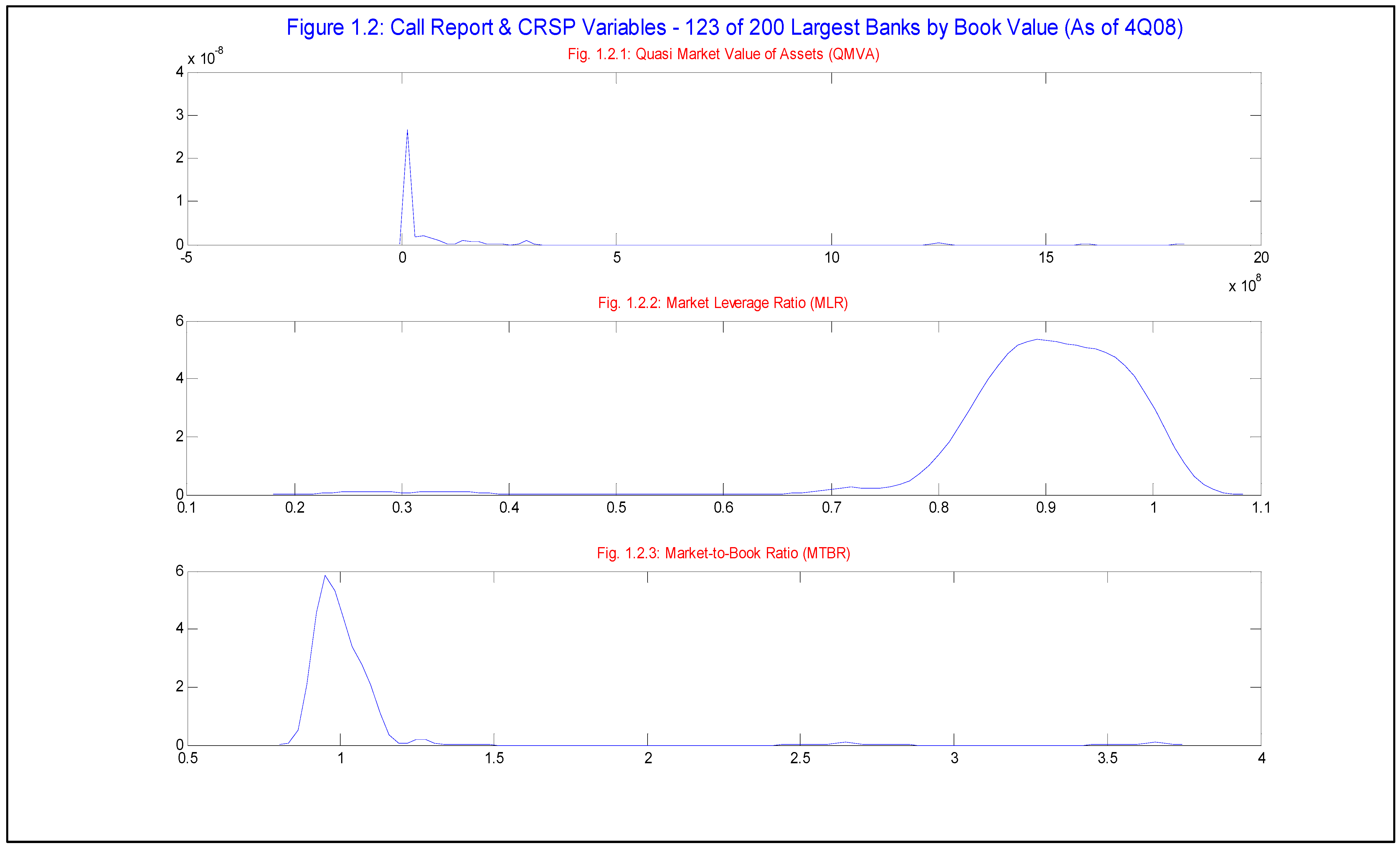
We gather equity price information from the Center for Research in Security Prices (CRSP) database as of 4Q08, extracting firms defined as financial institutions. In Table 1.2 and Figures 1.2.1-1.2.3, we summarize some equity market information for the banks in our sample, 123 of the Top 200 (which includes all the Top 5) for which we could make a definitive match to CRSP. This sample of banks for which we have equity price data (the “Top 123 CRSP”) allows us to compute various economically meaningful quantities, such as the “market leverage ratio” (defined as the ratio of the book value of total debt to itself plus the market value of equity – “MLR”), or the market-to-book ratio (defined as the ratio of the sum of the book value of total debt plus the market value of equity to the book value of assets - “MTBR”). We observe that the distributions of BLR and MLR are quite similar in the broader sample: respective medians of 90.3% and 90.7%. However, most of the Top 5 are somewhat more leveraged according to the MLR measure, ranging in 91.1% (WELLS) to 97.1% (CITI) by this metric, as compared to 91.31% (PNC) to 92.3% (CITI) for the BLR. This is reflective of the beating that the stocks of the largest banks had been subject to by year-end 2008. It is also worth noting that the Top 5 generally sell at a discount to book value according tom the MTBR, and lag the broader Top 123 CRSP sample where median (average) MTB is 98.8% (103.0%), and the Top 5 ranges from 95.1% (CITI) to100.4% (WELLS).

Table 1.3 and Figures 2 through 5 summarize distributional properties of and correlations amongst our 5 accounting based proxies for corresponding risk types. These calculated from quarterly Call Reports in the period 1Q84-4Q08, for the AT200 and Top 5 banks. We measure credit risk (“CR”) as gross charge-offs (“GCO”). We measure operational risk (“OR”) as other non-interest expense (“ONIE”). Market risk (“MR”) is proxied for by the deviation to the trailing 4-quarter average in net-trading revenues (“NTR-4QD”); such a measure is discussed in Jorion (2006). Whereas our proxy to CR of GCO is the same as in Rosenberg and Schuermann (2006), we deviate from that in estimating OR and MR, for which the authors used external operational risk data and a GARCH factor model fit to macro data, respectively. In our extension of capturing Liquidity Risk (“LR”) and Interest Rate (or Income) Risk (“IR”), we also follow the Jorion (2006) prescriptions. LR is approximated by the liquidity gap, defined as total loans minus total deposits, as a deviation from a moving 4-quarter trailing average ("LG-4QD"). Similarly, IR is approximated by the interest rate gap, defined as total interest expense minus total interest income, as a deviation from a moving 4-quarter trailing average ("IRG-4QD").

First considering quarterly GCO, we observe in Table 1.3 that median quarterly GCO ranges from $1.00B-$1.91B amongst the 4 largest of the Top 5, with PNC much lower at $270M. The range over time across the Top 5 is wide from $10M to $5.81B. In all cases GCO exhibits high positive skew. Median (mean) GCO for the AT200 is $6.66B ($7.89B), with a wide range of $1.92B to $31.16B, and significantly positive excess skewness. Median NIE ranges in $2.90B-$4.08B amongst the 4 largest of the Top 5, with PNC much lower at $84M. The range over time across the Top 5 is wide from $42M-$33.1B. In the case of 4 out of 5 of the 5 largest banks, GCO exhibits high positive skew, the exception being PNC. Median (mean) NIE for the AT200 is $6.66B ($7.89B), with a wide range of $1.92B to $31.16B, and significantly positive excess skewness. Median NTR-4QD ranges in $-88M to $4.08B amongst the Top 5. The range over time across the Top 5 is wide in -$0.88M to $9.09B. In the case of 4 out of 5 of the 5 largest banks, NIE exhibits high positive skew, with the exception of PNC. Median (mean) NTR-4QD for the AT200 is -$130M (-$10M), with a wide range of -$7.20B to $16.13B, and significantly positive excess skewness. Median LG-4QD ranges in -$6.85B to -$760M amongst the Top 5. The range over time across the Top 5 is wide in -$82.9B to $90.05B. LG-4QD exhibits less excess positive skewness than the other variables. Median (mean) LG-4QD for the AT200 is -$20.5B (-$20.1B), with a wide range of -$159.7B to $375.8B, and significantly positive excess skewness. Median IRG-4QD ranges in -$910M to $920M amongst the Top 5. The range over time across the Top 5 is wide in -$35.0B to $31.7B. Unlike the other variables, IRG-4QD exhibits mild negative skewness. Median (mean) IRG-4QD for the AT200 is -$2.62B (-$7.34B), with a wide range of -$171.72B to $153.01B, yet not having significantly negative excess skewness.

In Figure 2.1.1 through Figure 2.1.6 are displayed the smoothed kernel distributions of historical losses for each risk type, our accounting based proxies. We observe from these figures that indeed there is wide variation in the distributional properties of the different risk types. In the case of GCO, for AT200 and for all of the Top 5, we see the familiar right skewed and long tailed distribution of historical credit losses, as well as of theoretical loss distributions such as the Basel asymptotic single risk factor model. In some case however, we observe bi-modality, such as for JPMC and CITI. The distribution of ONIE, the OR proxy, is similarly non-negative and right-skewed with an elongated tail. Additionally, the mode appears shifted rightward relative to that of GCO (and not as peaked), the tails appear somewhat heavier and do not exhibit the multi-modality as in the distribution of GCO. On the other hand, the proxies for MR, LR and IR are all symmetric. However, there are subtle differences amongst these that are worthy of note. NTR-4QD exhibits the greatest degree of peakedness amongst these, while IRG-4QD the least. In the lower-left panel for each of these we show the distribution of the proxy for “Total Risk”, which is simply the sum of the 5 proxies. These are generally closer to symmetric than GCO and ONIE, but are heavier tailed and more skewed to the right than the remaining 3 proxies.

Given these distributional features, when we implement the copula models, we choose to model the marginal distributions of GCO and ONIE as 2-paramter GEV (equations 3.2.15 and 3.2.16), having non-negative support; and that of the remaining risk proxies (NTR-4QD, LG-4QD and IRG-4QD) as Student’s T distributions (equations 3.2.17), symmetric and with degrees of freedom determined by the data. We could fit alternative marginal distributions, potentially giving a better fit to the empirical distributions or better modeling the tails30, but we wish to make the simplest parametric choices possible that are still conservative, in that these exhibit heavy tails relative to normal or log-normal. This is for the purpose of making this exercise easily replicable by practitioners.

In Figure 2.2.1 through Figure 2.2.6 are displayed the quarterly time series of historical losses for accounting loss proxies of each risk type. We observe from these figures that indeed there is wide variation in the time series properties of the different risk types. In the case of GCO, for AT200 and for all of the Top 5, we see the familiar long cycling characteristic of annual loss rates in rating agency publications. In particular, note the peaks during the downturns of the early 1990’s and 2000’s, as well as most recently at the end of 2008 during the height of the financial crisis. It is more difficult to detect the cyclical effect in the time series of the OR proxy ONIE, and there appear to be greater differences across banks. In the case of AT200 and 3 of the Top 5, something like a smooth upward trend is evident, but not so for WELLS and PNC. In aggregate and across the most of the Top 5, the MR proxy NTR-4QD appears to fluctuate mildly around zero, with the exception of JPMC where the degree fluctuation is greater and appears to be increasing over time. And in all cases, there is an upward blip in the MR measure sometime in 2008, which is (with the exception of JPMC) a change of historically unprecedented magnitude. LG-4QD seems to lie somewhere between GCO and NTR-4QD in its time series behavior, having more variation over time than the latter, and faintly some of the long cycling of the former. One can see slight elevation in the liquidity risk measure in the last downturn and recently for JPMC, BofA and WELLS. On the other hand, IRG-4QD behaves quite differently than the other risk proxies, in all cases exhibiting very clear autocorrelation, having a saw-tooth pattern with much greater variability than but with no detect sensitivity to the cycle nor any discernable “blip” as compared with NTR-4QD. However, in most cases we can detect that the variability in this measure has mildly decreased over time (especially from early on in the sample period), possibly reflecting then use of derivatives on the part of banks to better manage this risk.

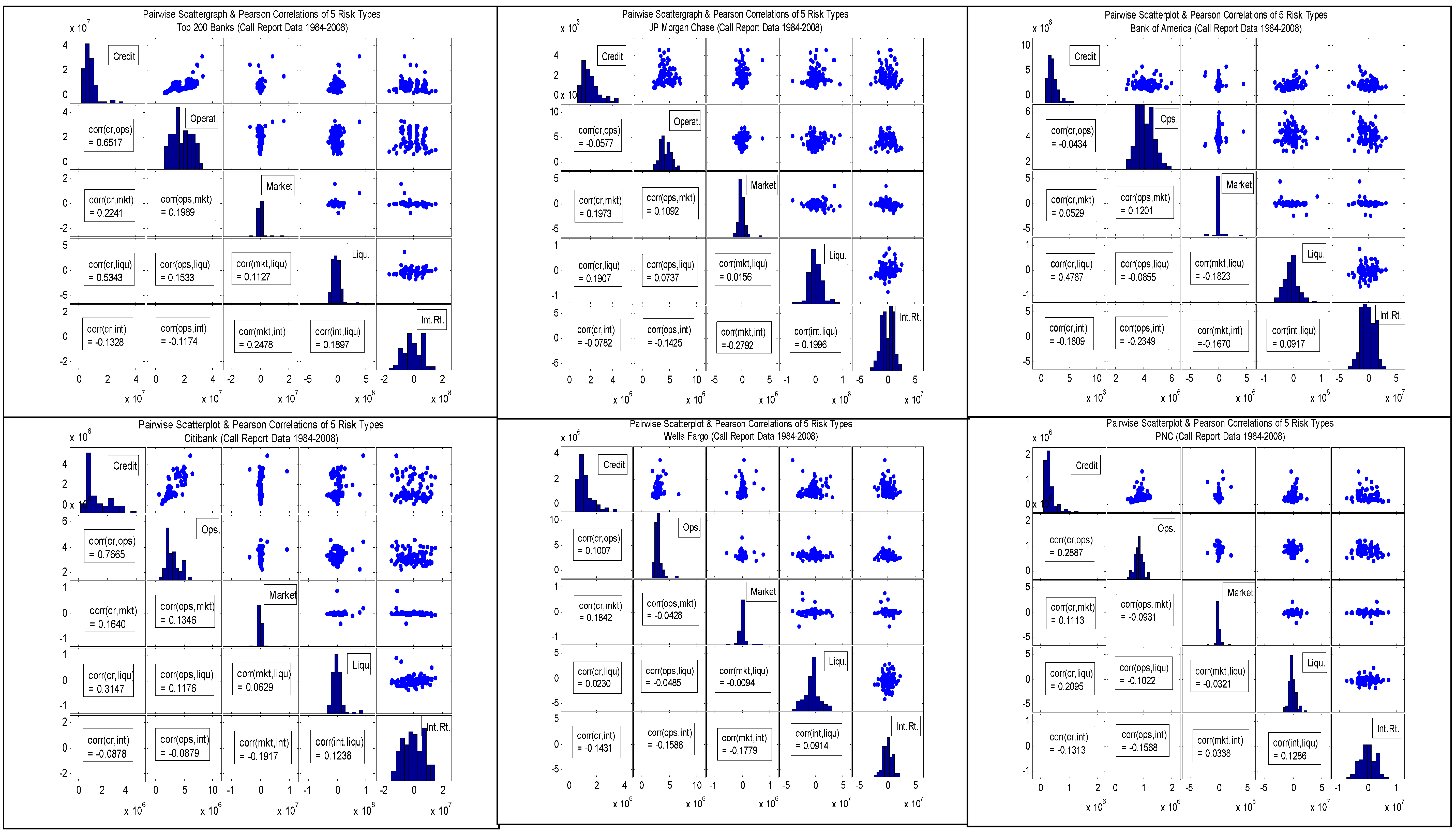
In Table 1.4, and in Figure 3.1 through Figure 3.6 (Figure 4.1 through Figure 4.6), we show the linear Pearson (rank-order Spearman31) correlations amongst the 5 proxies of the risk types. First, we observe some wide disparities across banks in the signs and magnitudes of the correlations. The second general observations is that magnitudes are generally on the low side, and in some cases negative, which would support the presence of substantial diversification benefits. Finally, the Spearman rank order correlations also exhibit wide disparity in signs and magnitudes across risk pairs, and moreover are not in generally in-line with the results of the linear correlation analysis.

In the case of CR and OR, Pearson correlations range from large and positive (0.65 and 0.77 for AT200 and CITI, respectively), to modest and positive (0.10 and 0.29 for WELLS and PNC, respectively), and then to small and negative (-0.06 and -0.04 for JPMC and BofA, respectively). The Spearman correlations are the same in sign and generally close to the Pearson correlations in magnitude for this pair, albeit significantly larger for PNC (41%). This runs counter to some empirical evidence that operational and credit risk losses may be positively correlated (Chernobai et al, 2008). Possibly this reflects the heterogeneity in control processes across banks that are better captured in this analysis.

In the case of CR and MR, in almost all cases Pearson correlations are positive and of modest magnitude, ranging from 0.16 (CITI) to 0.22 (AT200) in the 4 out of 5 cases, but is only 0.05 (0.09) for BofA (PNC). The Spearman correlations are close in most cases, except that it is negative (much smaller) for AT200 (CITI), -0.05 vs. 0.22 (0.08 vs. 0.16). These observations may be considered in line with empirical evidence and theoretical arguments that support a positive correlation between credit and market risks (Jarrow and Turnbull, 2000).

While CR and LR are all positively correlated by the Pearson measure, we observe that the magnitudes vary widely across banks: from large (0.53 and 0.48 for AT200 and BofA, respectively), to modest (0.19, 0.31 and 0.21 for JPMC, CITI and PNC, respectively), and to small (0.02 for WELLS). However, Spearman correlations agree neither in sign nor magnitude, being negative and small to modest in most cases: -0.12, -0.17, -0.03, -0.15 and -0.15 for JPMC, BofA, CITI, WELLS and PNC, respectively; only in the case of AT200 do we get a positive sign on the Spearman correlation, but of diminished magnitude (0.10) relative to the Pearson (0.53). Again, this is partly consistent with various empirical studies and models which have found or purport a positive relationship between credit and liquidity risk (Ericsson and, 2005), as well as certain theoretical models (Cherubini and Lunga, 2001.)

In the case of CR and IR, Pearson correlations are all negative, ranging in magnitude rather narrowly from small (-0.08 and -0.09 for JPMC and CITI, respectively) to modest (-0.13, -0.18, -0.14 and -0.13 for AT200, BofA, WELLS and PNC, respectively). But again we are in a situation in which the Spearman correlations are radically different, all positive and of relatively large, ranging from 0.17 to 0.33. While certain credit risk models in the structural class suggest a negative correlation (Merton, 1974), empirically we do not have a firm sense a priori of what the sign on this correlation ought to be.

In 4 out of 6 cases, OR and MR have modest positive Pearson correlations, ranging from 0.11 for JPMC to 0.20 for AT200, but are negative and have small (modest) values of -0.04 (-0.09) for WELLS (PNC). The Spearman correlations are also positive in most cases, but of diminished magnitude, ranging from 0.01 for WELLS to 0.10 for both JPMC and BofA; but as in the Pearson measure it is still negative for PNC (-0.07). There is really no empirical evidence of theory that can guide us in forming a prior on what the sign of this correlation should be. One may speculate that during market dislocations, strains on systems and personnel may increase the likelihood of an operational risk event, such as a trading error or the revelation of a fraud (e.g., see Jorion 2006 for the Barrings and Daiwa case studies).

Considering the Pearson correlation between our proxies for OR and LR, we see much diversity in sign and magnitude, while the Spearman correlations are all negative and of modest size. In the cases of JPMC, CITI and AT200 we observe Pearson correlations of small to modest magnitude (0.07, 0.12 and 0.15, respectively). On the other hand, the respective negative Pearson correlations of -0.05, -0.09 and -0.10 for WELLS, BofA and PNC tend to lie on the low range. The Spearman correlations are all negative and range from small (-0.02 for AT200) to modest (-0.24 and -0.26 for BofA and WELLS, respectively). Here we not only don’t have any research precedent to go on, but cannot offer much in the way of speculation about what the sign should be. It may very well be that during periods of a liquidity crunch internal controls are tightened in order to maximize available sources of funds, thereby mitigating the likelihood of an operational risk event, implying a negative relationship. Similarly, to the extent that liquidity may be more favorable during times of favorable credit quality or rising markets, when internal controls may be lax, this also supports a direct relation. And further supporting a positive dependence, we can imagine that the onset of an adverse operational loss may precipitate a loss of liquidity for a bank, which supports a direct relationship.

All of the Pearson correlations between OR and IR are negative and generally modest in magnitude: -0.09, -0.12, -0.14,-0.16, -0.16 and -0.23 for CITI, AT200, JPMC, WELLS, PNC and BofA, respectively. But the Spearman correlations are split in sign between positive (0.07, 0.10 and 0.12 for AT200, JPMC and CITI, respectively) and negative (-0.30, -0.05 and -0.04 for BofA, WELLS and PNC, respectively). Again here it is challenging to explain what these result should be. One may speculate that to the extent operational losses may occur in periods where bank margins are healthier (and not necessarily in economic upturns or good parts of the credit cycle) and controls are lax, the positive correlations observed in some cases may make sense.

We observe a wide range of in the signs and magnitudes of the Pearson correlations between MR and LR, while in 4 out of 6 cases Spearman correlations are moderately sized and negative. AT200 (BofA) has a modestly sized positive (negative) Pearson correlation of 0.11 (-0.18), and CITI (PNC) has a small positive (negative) correlation of 0.06 (-0.03), while JPMC (WELLS) has an insignificant positive (negative) correlation of 0.02 (-0.01). On the other hand, JPMC, BofA, CITI and WELLS have substantial negative Spearman correlations of -0.36, -0.23, -0.23 and -0.25, respectively; while AT200 and PNC stand out by this measure with insignificant positive correlations of 0.02 and 0.002. We find the Pearson results a little surprising, since it may be natural to think that liquidity measures would tend to be higher during downward market moves, as is more consistent with the Spearman measure results.

In the case of the MR-IR pair, the Pearson correlations are generally negative, while the Spearman correlations are for the most part positive. While for AT200 the Pearson correlation between MR and IR is positive and reasonably large (0.25), in the case of 4 out of the Top 5 it is moderately negative: -0.28, -0.19, -0.18 and -0.17 for JPMC, CITI, WELLS and BofA, respectively. And for the smallest of the Top 5, PNC, it is insignificantly positive at 0.03. But the Spearman measures tell a slightly different story: ranging from modestly (0.19 for AT200) to small (0.07 and 0.09 for WELLS and BofA, respectively) and positive on the one hand, to negative in one case (-0.09 for JPMC) and insignificant and positive in another (0.04 for PNC). Therefore, by the Pearson measure we observe that for the very largest of banks, adverse moves in our market risk proxy tend to coincide with favorable shocks to our interest rate risk measure. A possible explanation is that in periods of down markets, banks benefit from rising credit spreads on its loan book, while the rate on deposits is lagging. But we are not seeing this in the Spearman measure of dependence.

Finally, the correlation between IR and LR is consistently positive for both measures of correlation. In the Pearson case, these range from small (0.09 for both BofA and WELLS) to moderate (0.12, 0.13, 0.19 and 0.20 for CITI, PNC, AT200 and JPMC, respectively). The Spearman correlations are similar, albeit slightly larger: 0.08, 0.13, 0.15, 0.18, 0.21 and 0.26 for WELLS, AT200, BofA, PNC, JPMC and CITI, respectively. As with many of these results, we have little to go on in the way of prior expectations other than reasoned speculation. It is possible that in periods in which deposits are growing faster than expansion in loans happen to coincide with periods in which banks are competing for deposits, and hence the interest rate gap is widening.

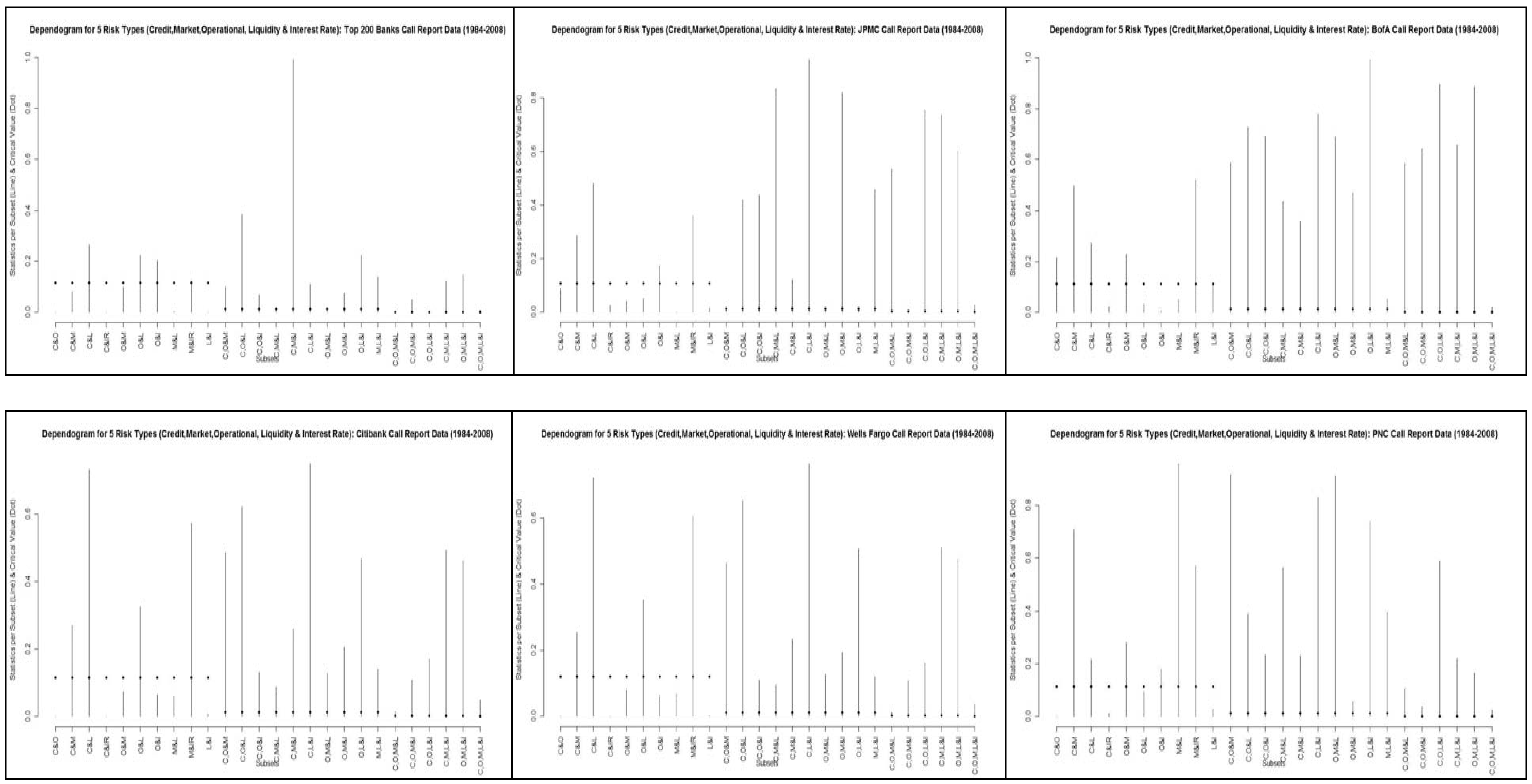
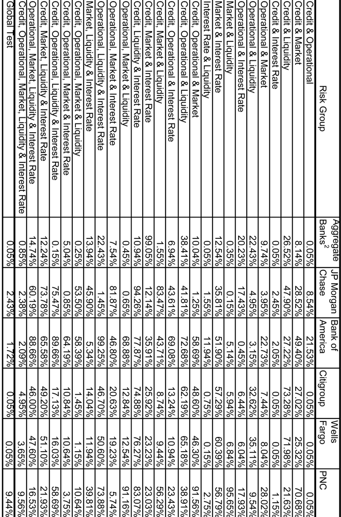
In Table 1.5 and in Figures 5.1-5.6 we present results group-wise tests of multivariate stochastic independence amongst our risk proxies developed by Genest et al (2004, 2009). The p-values of Table 1.5, derived under the null-hypothesis of independence with respect to each group, are based upon a comparison to the empirical copula process. Figures 5.1-5.6 are the dependograms of the test statistics and the corresponding critical values32. We find that across all the possible 26 sub-sets and 6 entities under consideration, in the majority of cases we fail to reject independence. For example, in only 14, 10, 5, 9, 9 and 6 groups do we reject the null hypothesis of independence at better than the 10% level for Top 200, JPMC, BofA, CITI, WELLS and PNC, respectively. At better than the 1% level, this drops off dramatically: 8, 3, 1, 3, 3 and 1 groups for the Top 200, JPMC, BofA, CITI, WELLS and PNC, respectively. It seems that we are able to reject independence in the most cases for Top 200, and the least for either BofA or PNC. However, in the case of the broad tests of the 5 risk types together in the second to last row, as well as the global test of at least one subset being independent in the final row, in all cases we are able to reject at the 10% level or better for all banks.

5.  ESTIMATION RESULTS: INTEGRATED RISK THROUGH ALTERNATIVE AGGREGATION METHODOLOGIES

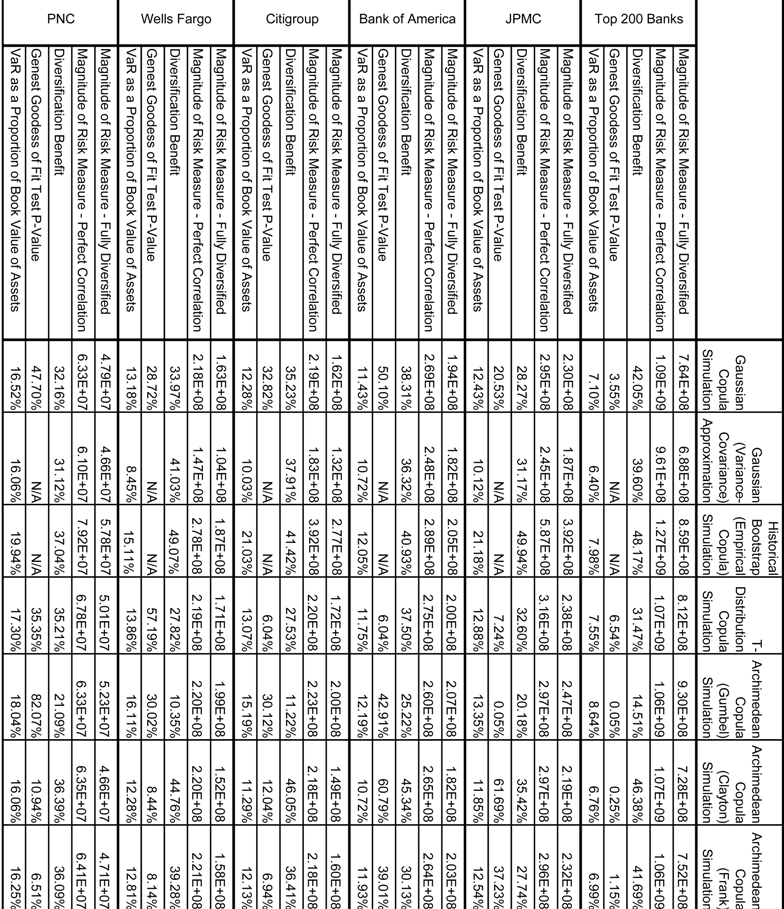
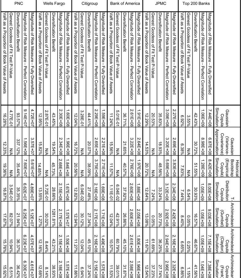
The main results of this paper are tabulated in Table 2.1, Table 2.2, Table 3.1 and Table 3.2; and shown graphically in Figures 6.1-7. In Table 2.1 we report the 99.97^th percentile VaR (Equation 3.1.2) for alternative risk aggregation methodologies for each AT200 and the Top 5 in row-wise panels, and in Table 2.2 we replicate this for the Expected Shortfall (ES) at the 99^th percentile (Equation 3.1.3). The different techniques are arrayed by column as “Gaussian Copula Simulation” (Equations 3.2.6-3.2.8; henceforth "GCS") 33, “Gaussian (Variance-Covariance) Approximation” (Equations 3.2.6-3.2.8; henceforth "VCA"), “Historical Bootstrap (Empirical Copula) Simulation” (Equation 3.2.9; henceforth "ECS"), “T - Copula Simulation” (Equation 3.2.8 henceforth "TCS"), “Archimadean Copula (Gumbel) Simulation” (Equation 3.2.13; henceforth "AGCS"), “Archimadean Copula (Clayton) Simulation” (Equation 3.2.12; henceforth "ACCS") and “Archimadean Copula (Frank) Simulation” (Equation 3.2.14; henceforth "AFCS"). The 1^st row in each panel labeled “Magnitude of Risk – Fully Diversified” represents the 99.97^th percentile (ES at the 99^th percentile) of the loss distribution, either simulated in the case of the copula methods or analytic in normal approximation, in Table 2.1 (Table 2.2). The second rows of each panel labeled “Magnitude of Risk – Perfect Correlation” represents the simple sum of the 99.97^th percentiles (ES at the 99^th percentile) of the simulated loss distributions for each risk type in the case of the copula methods, or the sum of the standard deviations of the loss in the analytic normal approximation (in either case, “simple summation” of risks), in Table 2.1 (Table 2.2). In the corresponding 3^rd rows we show the “Proportional Diversification Benefit” (henceforth PDB), which is defined as the difference in the risk measure between the perfect correlation and fully diversified cases, expressed as a proportion of fully diversified VaR or ES for the respective tables:

$$\text{\%\hspace{0.17em}}DiversificationBenefit{}^{Va{R}_{99.97\text{\%}}}=\frac{Va{R}_{PerfectCorrelation}^{Va{R}_{99.97\text{\%}}}-Va{R}_{FullyDiversified}^{Va{R}_{99.97\text{\%}}}}{Va{R}_{FullyDiversified}^{Va{R}_{99.97\text{\%}}}}$$

(30)

$$\text{\%\hspace{0.17em}}DiversificationBenefit{}^{E{S}_{99.9\text{\%}}}=\frac{Va{R}_{PerfectCorrelation}^{E{S}_{99.9\text{\%}}}-Va{R}_{FullyDiversified}^{E{S}_{99.9\text{\%}}}}{Va{R}_{FullyDiversified}^{E{S}_{99.9\text{\%}}}}$$

(31)

In the second-to-bottom rows we tabulate the p-values of the Genest and Remillard (2009) goodness-of-fit tests for the copula models. Approximate p-values for this test are based upon the a comparison of the empirical copula (EC) to a parametric estimate of the copula in question, that is generated through a parametric bootstrap, under the null hypothesis the data is generated through the EC process34.

In the bottom row of each panel in Table 2.1 and Table 2.2 we show the diversified VaR and ES as a proportion of the book value of total assets (BVTA), for AT200 and each Top 5 institution as of the year-end 2008. We observe wide variation in all risk and diversification measures across aggregation methodologies for a given institution, as well as across banks for a given technique.

First we shall discuss the VaR results in Table 2.1. The dollar VaR (shown graphically in Figure 6.1) is increasing in size of institution, ranging cross diversification methodologies: $688B-$930B for AT 200, $187B-$392B for JPMC, $182B-$207B for BofA, $132B-$277B for CITI, $104B-$199B for WELLS, and finally a big drop-off $46.6B-$57.8B for PNC. We show these graphically in Figure 5.1.

VaR expressed as a proportion of BVA (shown graphically in Figure 2.2) also shows much variation across both aggregation techniques and institutions, ranging from the mid single-digits to just below 20%. These percentages generally decrease with the size of the institution, although the relationship is not strictly monotonic. We observe percentages lowest for the hypothetical aggregate AT200 (6%-9%), highest for PNC (16%-18%), and generally hovering just north of 10% for the middle 4 banks: 10%-20%, 11%-12%, 10%-15%, 8%-16% for JPMC, BofA, CITI and WELLS, respectively. Note that the ranges of VaR/BVA across methodologies appear to be increasing from JPMC down to WELLS. We are cautious to conclude much from this, such as a “business line diversification story”, due to the small sample size. Comparing different risk aggregation methodologies across banks, we observe that VCA produces consistently the lowest VaR, and that either the ECS or the AGCS produce the highest VaR, across all institutions. ECS and ACGS is followed by TCS in terms of conservativeness, while the GCS “benchmark” is usually somewhere in the middle, and ACCS is toward the low side. AFGS tends to be closest to GCS, albeit usually just a little lower. While TCS is always higher than GCS, in some cases it is not by a very wide margin.

In the case of AT200, VaR under ECS (VCA) is $859B ($688B), $392B ($187B), $205B ($182B), $277B ($132B) , $187B ($104B) and $57.8B ($46.6B) for AT200, JPMC, BofA, CITI, WELLS and PNC, respectively; and this brackets the respective GCS VaRs of $764B, $230B, $194B, $162B, $163B and $47.9B. AGCS is in some cases close to ECS, and in others still higher than GCS (understandably, with the property of upper tail dependence), with VaRs of $930B, $247B, $207B, $200B, $199B and $52.3B for AT200, JPMC, BofA, CITI, WELLS and PNC, respectively. On the other hand, TCS is always higher than GCS, but in some cases by only a modest amount (and generally less than AGCS or ECS): VaRs of $812B, $238B, $200B, $172B, $171B and $50.1B for AT200, JPMC, BofA, CITI, WELLS and PNC, respectively. The ACCS is generally second-place to VCA in lack of conservativeness, understandably so given its property of lower tail dependence: VaRs of $728B, $219B, $182B, $149B, $152B and $46.6B for AT200, JPMC, BofA, CITI, WELLS and PNC, respectively. Finally, we see that the AFCS (the Archimadean copula characterized by neither upper nor lower tail dependence) is middling and often close to GCS in VaR magnitude as compared to its brethren methodologies: VaRs of $752B, $232B, $203B, $160B, $158B and $47.1B for AT200, JPMC, BofA, CITI, WELLS and PNC, respectively.

The proportional diversification benefits, or PDBs (shown graphically in Figure 6.3), exhibit a great deal variation across banks and aggregation techniques, range from 10% to 50%, with the ECS (AGCS) yielding clearly higher (lower) values than the other methodologies. PDBs ECS ranges in 40% to 50%, while they range in 10% to 25% for AGCS. Across banks, the GCS “benchmark” tends to lie in the middle (41-58%), and the VCA to the lower end of the range (31-41%), while AGCS is the lowest (10-21%).

Looking at the range of the PDBs across aggregation methodologies for a given bank, we attempt to measure the impact of business mix. However, we cannot observe a directionally consistent pattern. The 2 banks with the highest proportion of trading have diversification benefits lying in a low and wide (11.2% to 46.1% for CITI) to a high and narrow range (20.3% to 36.6% for JPMC). On the other hand, considering banks with proportionately more lending assets, BofA has a range similar to JPMC (25.2% to 38.3%), while Wells and PNC more closely resemble CITI (10.4% to 49.1% and 21.1% to 37.0%, respectively). We shall not discuss the 99th percentile expected shortfall (ES) results in Table 2.2, as generally the results are quite in both absolute quantities and in comparisons across institutions or aggregation methodologies.

The results of the Genest et al (2009) GOF tests (shown graphically in Figure 6.4) are highly mixed (we reject the null in just under one-half of cases, 14 out of 30) and do not lend themselves to the extraction of a clear pattern. Generally, the rejections of fit to the empirical processes are not at very high levels of significance, so that perhaps we can say that the models are doing a decent job. There are only 3 rejections at better than the 1% level (AGCS for AT200 and JPMC, AGCS for JPMC), only one at the 5% level (AFCS for AT200), and the remaining 9 at only the 10% level (and in one case, the p-value is just above 0.10). AT200 has the most rejections (in all cases, models are rejected at the 10% level), followed by JPMC (2 rejections for TCS and AGCS), CITI and WELLS (2 rejections each at the 10% level), with BofA and PNC having the least (only 1 each at the 10% level). Across banks, the GCS and AGCS models fail to reject a fit to the data most often (1 and 2 rejections, respectively; however, AGCS has the 2 lowest p-value), while the TCS (4 at the 10% level) and AFCS (3 at the 10% level and 1 at the 5% level) have the most rejections.

The object of the second analysis that we perform, a bootstrap (or resampling) exercise, is to measure the uncertainty in the VaR and PDB estimates. This is now a widely used technique in finance and economics, originating mainly in the statistics literature, which has the potential to develop estimates of standard errors or confidence intervals for complex functions of random variables for which distribution theory is undeveloped (Efron and Tibshirani, 1986). The type of bootstrap that we implement is the so-called non-parametric version, in which the data is resampled with replacement. In each iteration, the function of interest is recalculated, yielding a distribution of the latter which can be analyzed. As the VaR estimate in any of the aggregation frameworks depends upon a random sample of observations, and in the case of the VCA or the copulas parametric estimates of the marginal distributions or of the correlation matrices, the uncertainty in the latter flows through to the former. This manner of analysis is of keen importance to regulators, as they must seek to understand how we may decompose the volatility of capital from year-to-year into that driven by the variability in model inputs, from that stemming from changes to a bank’s risk profile.

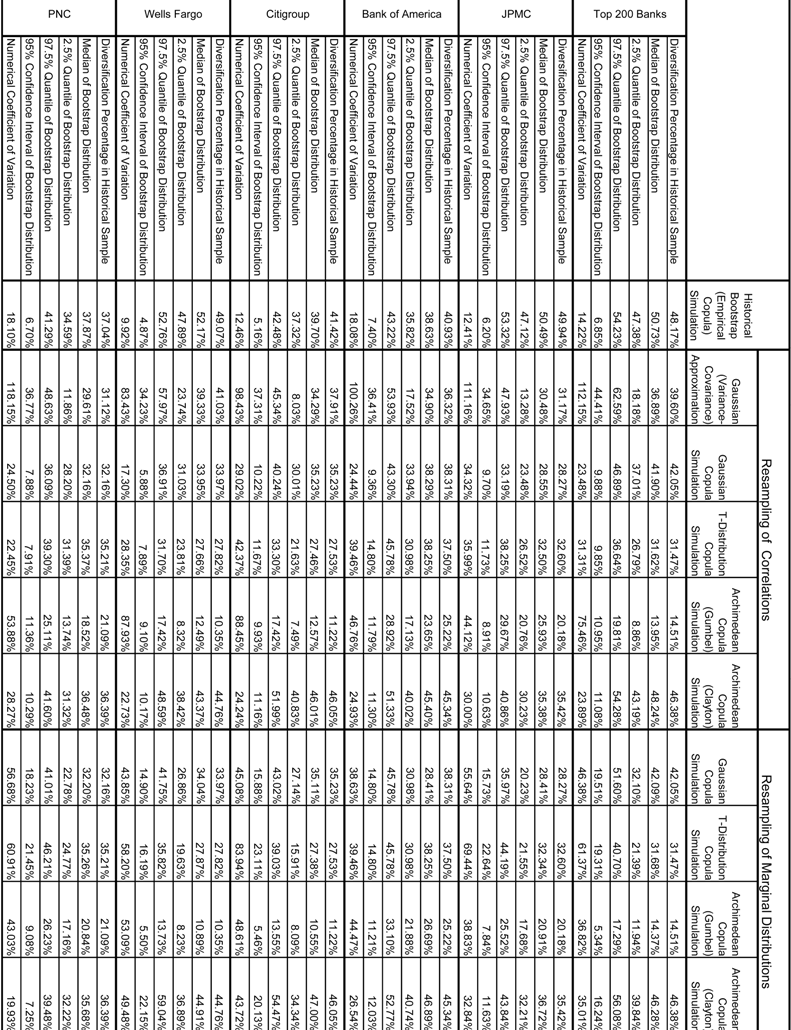
The results of this experiment are tabulated in Table 3.1 and Table 3.2 for the VaR and PDB estimates, respectively. We resample with replacement 10,000 times, and in each bootstrap we run a simulation of 100,000 years as in the main results. The numerical coefficients of variation (NCV) of VaR and PDB across banks and techniques are shown in the final rows of each panel in Table 3.1 and Table 3.2, as well as graphically in Figures 7.1-7.4. We define the NCV as the ratio of the 95% confidence interval in the bootstrapped sample to the estimate in the historical sample:

$$NC{V}_{95\text{\%}}^{Va{R}_{99.97\text{\%}}}=\frac{Va{R}_{BTSTR{P}_{Q97.5\text{\%}}}^{99.97\text{\%}}-Va{R}_{BTSTR{P}_{Q2.5\text{\%}}}^{99.97\text{\%}}}{Va{R}_{SMPL}^{99.97\text{\%}}}$$

(32)

$$NC{V}_{95\text{\%}}^{PD{B}_{99.97\text{\%}}}=\frac{PD{B}_{BTSTR{P}_{Q97.5\text{\%}}}^{99.97\text{\%}}-PD{B}_{BTSTR{P}_{Q2.5\text{\%}}}^{99.97\text{\%}}}{PD{B}_{SMPL}^{99.97\text{\%}}}$$

(33)

We do this bootstrap in two ways: holding the estimates of the marginal distributions constant, and re-estimating the correlations, and vice-versa (i.e., assuming that we know the true correlation matrix, but that the parameters the marginal distribution is measured with error), shown in the left and right panels of the tables, respectively. However, in the case of ESC, we cannot do either of these and simply draw a new sample from which we estimate an empirical copula from the resampled data. And in the case of the VCA, we can only do the correlation resampling, as that methodology does not depend upon fitting marginal distributions.

There are several clear conclusions that we can draw based upon these results. First, we fail to observe a consistent pattern in the variability of VaR or PDB across size or types of banks (i.e., business mix). Second, regarding which model is most or least stable, we observe that for either the bootstrap of VaR or PDB, the ECS and GSC techniques yields generally the lowest NCVs as compared to other methodology. Third, we see that in contrast to this, the VCA is consistently the most variable in the bootstrap, having for the most part the highest NCVs. In the comparison between VCA and the copula methods (excluding ECS) this is somewhat surprising, since VCA does not require estimation of marginal distribution parameters, yet nonetheless has much higher NCVs in the resampling of correlations for any of the copula methodologies. In the bootstrap of VaR, NCV ranges in 6.4%-13.6% for ECS and 27.9%-45.3% for VCA, while in the resampling of correlations (margins) for GCS they range in 7.1%-9.0% (35.4%-48.2%). Fourth, for either the bootstrap of VaR or PDB, NCVs are an order of magnitude higher for the resampling of margins as compared to the resampling or correlations, and this difference is accentuated for the bootstrapping of VaR as compared to PDB. Five, NCVs are higher for the PDB as compared to the VaR statistics. In the case of VaR, NCVs in the bootstrap of correlations (margins) range in 5.9%-45.3% (25.2%-69.6%), while in the case of PDB the corresponding numbers are 9.9%-158.2% (22.7%-118.2%). Finally, according to the NCV criterion, the PDB is much more imperfectly estimated than the VaR, across methodologies or banks.

In the case of the VaR bootstrapping in Table 3.1, the NCV for ECS is 8.1%, 6.4%, 13.6%, 9.1%, 9.1% and 8.9% for AT200, JPMC, BofA, CITI, WELLS and PNC, respectively. The corresponding NCV of VaR numbers for VCA in the bootstrap of correlations are much higher: 28.2%, 30.3%, 27.9%, 45.3%, 27.0% and 32.9%, respectively. However, in the case of GCS, the corresponding NCVs for the correlation bootstrap of VaR are slightly lower than ECS at 7.1%, 7.8%, 8.9%, 8.0%, 8.1% and 9.0% for AT200, JPMC, BofA, CITI, WELLS and PNC, respectively. In this exercise of varying the correlations, the NCVs of both the Student-T (8.5%, 7.5%, 11.1%, 12.0%, 16.4% and 10.9%) and AGCS (10.6%, 7.5%, 10.8%, 9.6%, 9.3% and 10.0%) slightly higher for AT200, JPMC, BofA, CITI,WELLS and PNC, respectively. Finally, ACCS is slightly lower in NCV across banks: 6.6%, 7.0%, 6.5%, 6.5%, 6.0% and 5.9% for AT200, JPMC, BofA, CITI, WELLS and PNC, respectively.

In the bootstrapping of margins for VaR in the right panel of Table 3.1, we observe that the NCVs of all the copula models are higher than VCA and far exceed ECS, but it is hard to tell which of these is consistently greater or less. In the case of GCS the NCVs for the margin bootstrap of VaR are 35.4%, 41.4%, 48.2%, 38.4%, 40.0% and 44.8% for AT200, JPMC, BofA, CITI, WELLS and PNC, respectively. The NCVs of Student-T are all higher than those for GCS: 43.6%, 46.6%, 56.1%, 62.2%, 46.0% and 47.4% for AT200, JPMC, BofA, CITI, WELLS and PNC, respectively. But the comparison to of GCS or TCS to either AGCS (39.3%, 33.5%, 37.8%, 52.7%, 45.7% and 44.9% for AT200, JPMC, BofA, CITI, WELLS and PNC, respectively) and ACCS (44.36%, 50.0%, 25.2%, 54.4%, 62.1% and 69.6% for AT200, JPMC, BofA, CITI,WELLS and PNC, respectively) is mixed across banks.

As with the VaR bootstrapping, in the resampling of PDB in Table 3.2, we observe that overall NCVs are higher than in the estimation of VaR, across methodologies and institutions. The estimation of PDB is least precise for VCA, and generally most accurate for ECS, followed closely by GCS in having low NCVs. In the resampling of correlations, the GCS and CCS are notably more variable, in that order, as compared with the VaR estimation. As with the case of VaR, the resampling of margins has higher NCVs, although the difference as compared to the correlation bootstrapping is not as stark as in VaR estimation.

In Table 3.2 for PDB in the resampling of correlations we observe that the NCV for ECS is 14.2%, 12.4%, 18.1%, 12.5%, 9.9% and 18.1% for AT200, JPMC, BofA, CITI, WELLS and PNC, respectively. The corresponding NCVs for GCS are significantly higher in most cases at 23.5%, 34.3%, 24.4%, 29.0%, 17.3% and 24.5%. The NCV of PDB numbers for VCA are much higher: 112.2%, 111.2%, 100.3%, 98.4%, 83.4% and 118.2% for AT200, JPMC, BofA, CITI, WELLS and PNC, respectively. In the exercise of varying the correlations, the NCVs of PDB is slightly higher for TCS than GCS (31.3%, 36.0%, 39.5%, 42.4%, 28.4% and 22.5% for AT200, JPMC, BofA, CITI, WELLS and PNC, respectively). On the other hand, AGCS is much higher than GCS or TCS in some cases: 75.5%, 44.1%, 46.8%, 88.5%, 87.9% and 53.9% for AT200, JPMC, BofA, CITI, WELLS and PNC, respectively. And ACCS is somewhere between GCS and TCS: 23.9%, 30.0%, 24.9%, 24.2%, 22.7% and 28.3% for AT200, JPMC, BofA, CITI, WELLS and PNC, respectively.

In Table 3.2 for PDB in the resampling of margins we observe that the NCVs for GCS are quite a bit higher than in the resampling of correlations, now 46.4%, 55.6%, 38.6%, 45.1%, 43.9% and 56.7% for AT200, JPMC, BofA, CITI, WELLS and PNC, respectively. While always higher, in contrast with the exercise of varying the correlations, the NCVs of PDB are in some cases much higher for TCS than for GCS: 61.4%, 69.4%, 39.5%, 83.9%, 58.2% and 60.9% for AT200, JPMC, BofA, CITI, WELLS and PNC, respectively. On the other hand, AGCS is now generally lower than TCS but not for from GCS: 36.8%, 38.8%, 44.5%, 48.6%, 53.1% and 43.0% for AT200, JPMC, BofA, CITI, WELLS and PNC, respectively. And ACCS is still somewhere between GCS and TCS: 35.0%, 32.8%, 26.5%, 43.7%, 49.5% and 19.9% for AT200, JPMC, BofA, CITI, WELLS and PNC, respectively.

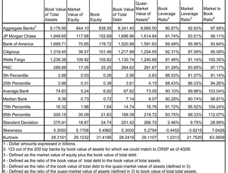
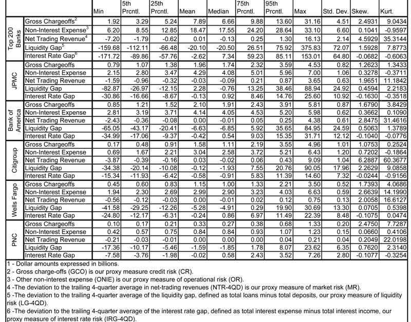
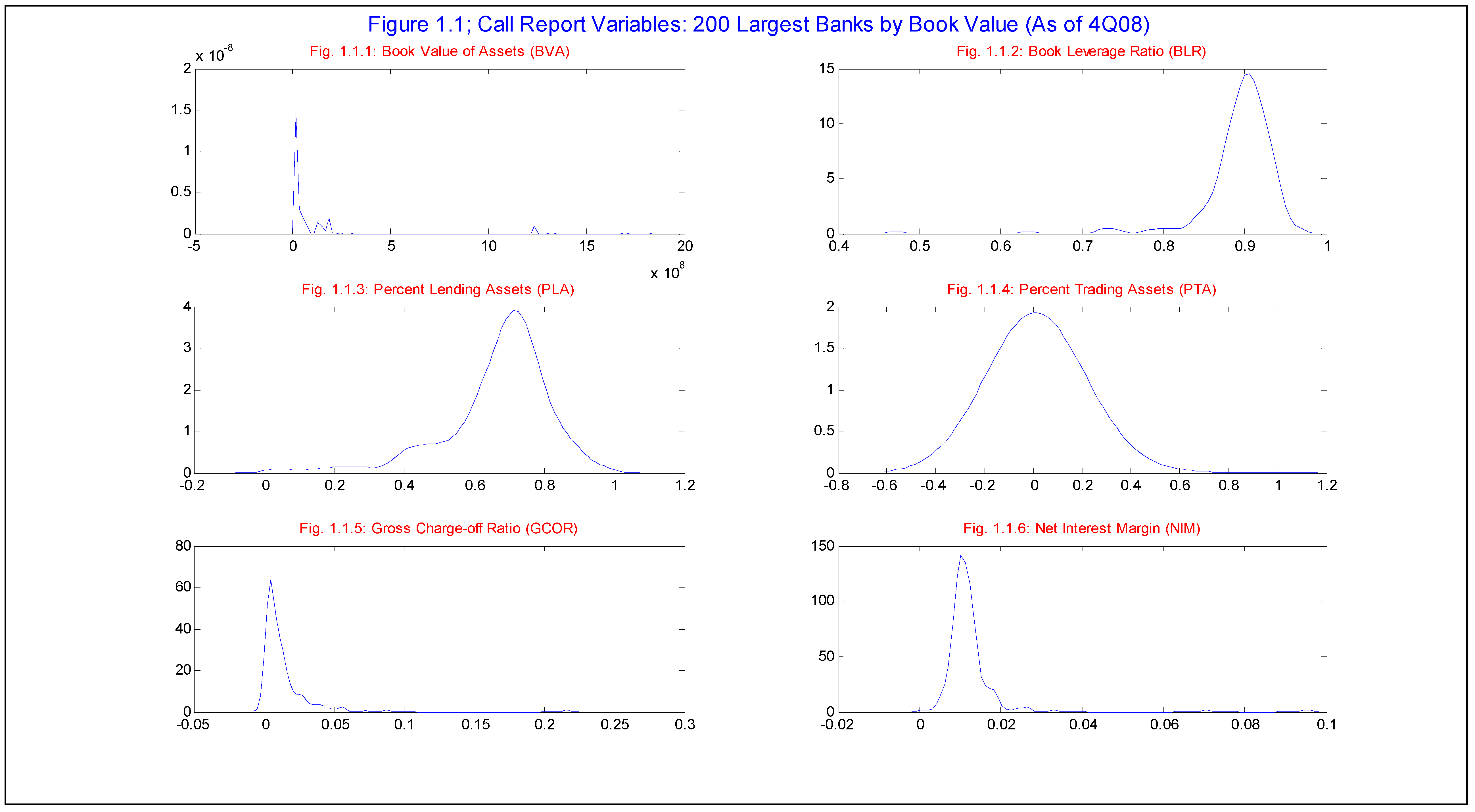
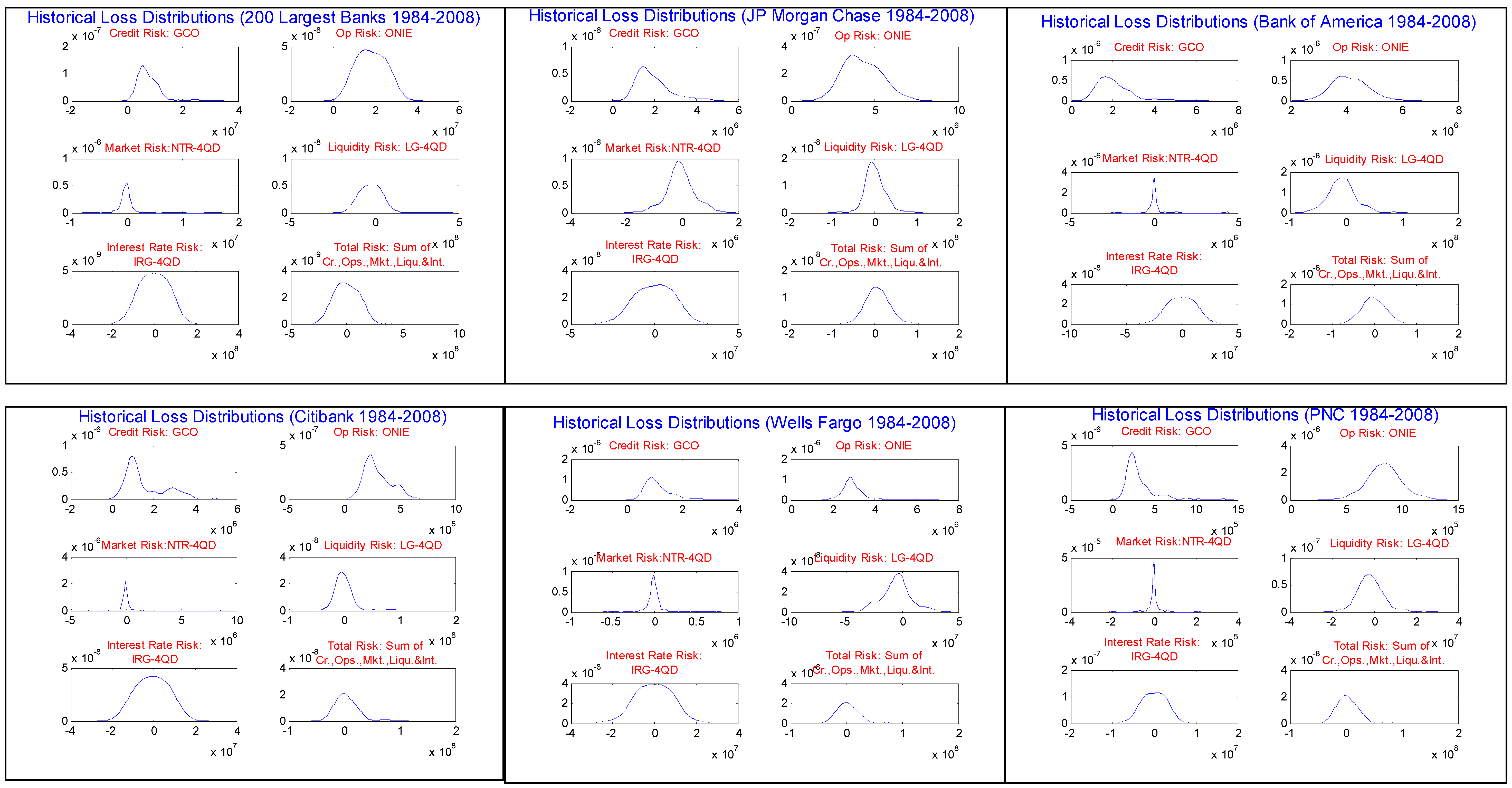
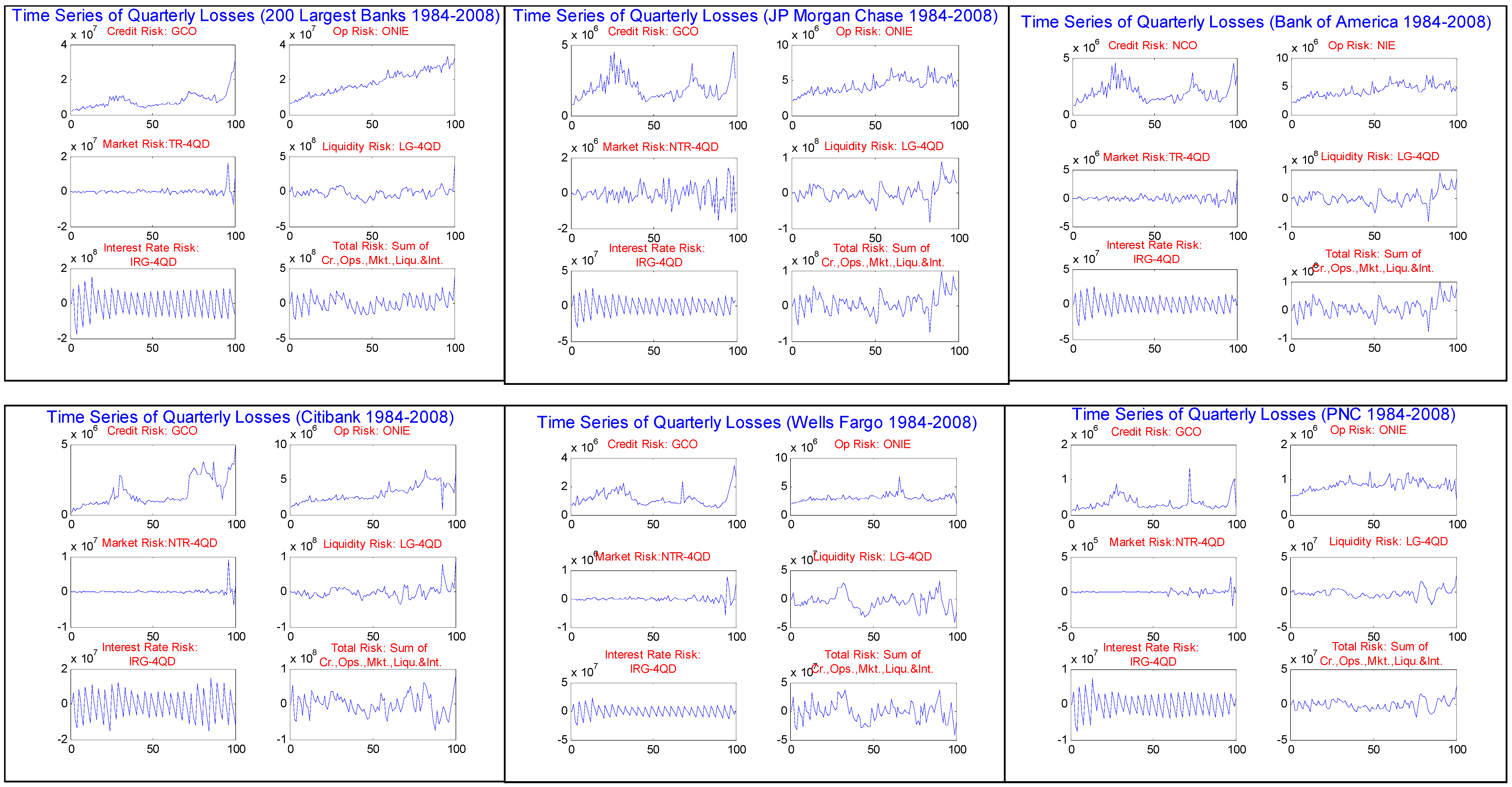6.  SUMMARY OF MAJOR CONCLUSIONS AND DIRECTIONS FOR FUTURE RESEARCH

In this study, we have compared alternative risk aggregation methodologies. We have described various models used in practice, including the variance-covariance approximation (VCA), as well as various copula simulations formulations that include the well-known parametric Gaussian copula simulation (GCS) and the less-well known (in this context) empirical copula simulation (ECS). Through differences observed across the five largest banks by book value of assets as of the end of 2008, proxying for five risk types using accounting data from Call Reports submitted to national supervisors, we have identified a range of results across different models for aggregating risk. The first major exercise involved fitting the models, describing and comparing value-at-risk (VaR) and proportional diversification benefits (PDBs) across banks and models, as well as goodness-of-fit statistics (GOF) for the latter. The second part involved measuring the statistical variation in the VaR and PDB measures through a non-parametric bootstrap.

First, while we documented that dollar 99.97^th percentile VaR is increasing in size of institution, VaR as a fraction of book value does not appear to be a monotonically increasing in size (however, it appears to decrease overall). Second, we saw that across different risk aggregation methodologies and banks that consistently the ECS and AGCS produce the highest absolute magnitudes of VaR as compared to either GCS “benchmark”, STCS or any of the other Archimadean copulas. Furthermore, ECS – a variant of the well-established “historical simulation” methodology in market risk practice – was in many cases found to be most conservative, a surprise in that according to asymptotic theory it should be the lower bound across copula models. On the other hand, the VCA consistently produced the lowest VaR number, which is disturbing in that several bank practitioners are (for the lack of theoretical or supervisory guidance) adopting this computational shortcut. Third, we also noted that the PDB tended to be largest for the ECS than the other methodologies, including the GCS “benchmark” or the VCA, while the AGCS produced the lowest. Therefore, if we regard ECS as a reasonable benchmark with much to recommend it, we caution that banks choosing either the VCA or other copula models may possibly understate diversifications benefits. Fourth, through differences observed across the two (three) of five largest banks having proportionately more trading (lending) assets, we failed to find business mix to exert a directionally consistent an impact on total integrated risk. Fifth, in an application of a blanket goodness-of-fit tests for copula models (Genest et al, 2009), we found mixed results: while in about half the cases commonly utilized parametric copula models fail to fit the data, confidence levels tended to be modest, so clearly this is an area that warrants further investigation and experimentation. Finally, the bootstrapping experiment revealed the variability of the VaR itself to be significantly lowest (highest) for the ECS and GCS (VCA) relative to other risk aggregation models. Furthermore, we found that the contribution of the sampling error in the parameters of the marginal distributions to be an order of magnitude greater than that of the dependency measures. Overall, our results constituted a sensitivity analysis that argues for practitioners to err on the side of conservatism in considering a non-parametric copula alternative in order to quantify integrated risk. This is because standard copula formulations produced a wide divergence in measured VaR, diversification benefits as well as the sampling variation in both of these across different measurement frameworks and types of institutions.

There are various fruitful avenues along which this research may be extended. First, motivated by some of our descriptive analysis (i.e., pairwise correlations and group-independence tests), we may want to model sub-sets of risk factors according to different dependency structures (e.g., different copula models). An ideal framework for accomplishing this is the pair-copula formulation (Aas and Berg, 2007). While this is computationally challenging, we believe the returns to be substantial, and at this point we are pursuing such an empirical strategy. Indeed, it may well turn out that this more realistic framework performs not only better than standard copulas, but beats the ECS model that this paper has found so robust. Second, we may consider alternatives to the copula paradigm, such as a dynamic time series model; an example that comes to mind is the dynamic conditional correlation (DCC) model of Engle and Sheppard (2001) and Engle (2002). Third, we may investigate alternative proxies for risk factors, or different risk factors themselves, in this or in a competing framework. Lastly, we could expand the universe of banks that we study (e.g., the Top 10 or 20 by assets size).

TABLES AND FIGURES

Table 1.1. Summary Statistics on Characteristics of Top 200 and 5 Largest Banks by Asset Size (Call Report Data As of 2008¹)

Table 1.1. Summary Statistics on Characteristics of Top 200 and 5 Largest Banks by Asset Size (Call Report Data As of 2008¹)

Table 1.2. Summary Statistics on Market Value Characteristics of Banks by Asset Size (Call Report and CRSP Data As of 2008¹)

Table 1.2. Summary Statistics on Market Value Characteristics of Banks by Asset Size (Call Report and CRSP Data As of 2008¹)

Table 1.3. Summary Statistics on Risk Measures for Top 200 and 5 Largest Banks by Asset Size (Call Report Data 1984-2008¹)

Table 1.3. Summary Statistics on Risk Measures for Top 200 and 5 Largest Banks by Asset Size (Call Report Data 1984-2008¹)

Table 1.4. Pairwise Correlations for Top 200 and 5 Largest Banks Risk Proxies (Call Report Data 1984-2008)

Table 1.4. Pairwise Correlations for Top 200 and 5 Largest Banks Risk Proxies (Call Report Data 1984-2008)

Table 1.5. Genest et al (2004) Mulivariate Groupwise Independence Test P-Values: Top 200 and 5 Largest Banks Risk Proxies (Call Report Data 1984-2008)

Table 1.5. Genest et al (2004) Mulivariate Groupwise Independence Test P-Values: Top 200 and 5 Largest Banks Risk Proxies (Call Report Data 1984-2008)

Table 2.1. 99.97% Confidence Level Value-at-Risk for 5 Risk Types: Credit, Operational, Market, Liquidity & Interest Rate (200 Largest Banks: Call Report Data 1984-2008)

Table 2.1. 99.97% Confidence Level Value-at-Risk for 5 Risk Types: Credit, Operational, Market, Liquidity & Interest Rate (200 Largest Banks: Call Report Data 1984-2008)

Table 2.2. 99.9% Confidence Level Expected Shortfall for 5 Risk Types: Credit, Operational, Market, Liquidity & Interest Rate (200 Largest Banks: Call Report Data 1984-2008)

Table 2.2. 99.9% Confidence Level Expected Shortfall for 5 Risk Types: Credit, Operational, Market, Liquidity & Interest Rate (200 Largest Banks: Call Report Data 1984-2008)

Table 3.1. Bootstrap Analysis of 99.97% Confidence Level Value-at-Risk for 5 Risk Types: Credit, Operational, Market, Liquidity & Interest Rate (200 Largest Banks: Call Report Data 1984-2008)

Table 3.1. Bootstrap Analysis of 99.97% Confidence Level Value-at-Risk for 5 Risk Types: Credit, Operational, Market, Liquidity & Interest Rate (200 Largest Banks: Call Report Data 1984-2008)

Table 3.2. Bootstrap Analysis 99.97% Confidence Percent Level Diversification Benefit for 5 Risk Types: Credit, Operational, Market, Liquidity & Interest Rate (200 Largest Banks: Call Report Data 1984-2008)

Table 3.2. Bootstrap Analysis 99.97% Confidence Percent Level Diversification Benefit for 5 Risk Types: Credit, Operational, Market, Liquidity & Interest Rate (200 Largest Banks: Call Report Data 1984-2008)

Figures 1.1.1-1.1.6. Distributions of Key Call Report Variables as of 4Q08 for Top 200 Banks by Book Value of Assets

Figures 1.1.1-1.1.6. Distributions of Key Call Report Variables as of 4Q08 for Top 200 Banks by Book Value of Assets

Figures 1.2.1-1.2.3. Distributions of Key Call Report Variables as of 4Q08 for Top 200 Banks by Market Value of Assets

Figures 1.2.1-1.2.3. Distributions of Key Call Report Variables as of 4Q08 for Top 200 Banks by Market Value of Assets

Figures 2.1.1-2.1.6. Kernel Density Estimated Distributions of Historical Losses

Figures 2.1.1-2.1.6. Kernel Density Estimated Distributions of Historical Losses

Figures 2.2.1-2.1.6. Quarterly Time of Historical Losses

Figures 2.2.1-2.1.6. Quarterly Time of Historical Losses

Figures 3.1-3.6. Pairwise Panel Scattergrams and Pearson Correlations of Risk Proxies

Figures 3.1-3.6. Pairwise Panel Scattergrams and Pearson Correlations of Risk Proxies

Figures 4.1-4.6. Pairwise Panel Scattergrams and Spearman Correlations of Transformed Risk Proxies

Figures 4.1-4.6. Pairwise Panel Scattergrams and Spearman Correlations of Transformed Risk Proxies

Figures 5.1-5.6. Genest et al (2009) Dependograms of Independence Tests

Figures 5.1-5.6. Genest et al (2009) Dependograms of Independence Tests

Figures 6.1-6.4. Dollar & Relative Value-at-Risk, Proportional Diversification Benefits and, Genest et al (2009) G.O.F. Test P-Values

Figures 6.1-6.4. Dollar & Relative Value-at-Risk, Proportional Diversification Benefits and, Genest et al (2009) G.O.F. Test P-Values

Figures 7.1-7.4. Coefficients of Variation of Bootstrapped Value-at-Risk and Percent Diversification Benefit across Methodologies and Banks

Figures 7.1-7.4. Coefficients of Variation of Bootstrapped Value-at-Risk and Percent Diversification Benefit across Methodologies and Banks