Performance of Pairs Trading Strategies Based on Various Copula Methods

Abstract

This study evaluates three pairs trading strategies—the distance method (DM), mispricing index (MPI) copula, and mixed copula—across the Chinese equity market from 2005 to 2024, incorporating time-varying transaction costs. To enhance computational efficiency, a novel two-step methodology is proposed that first selects candidate pairs based on the sum of squared differences and then applies copula models to capture nonlinear and asymmetric dependence structures between stocks. Pre-cost monthly excess returns are 84, 30, and 25 basis points, respectively, dropping to 81, 23, and 15 basis points post-costs. While the DM consistently delivers higher returns, copula strategies offer advantages in stability and resilience, especially in volatile markets. The Student-t copula proves particularly effective in capturing dependence structures with fat tails and asymmetric correlations. Although copula methods face challenges such as unconverged trades—instances where spreads fail to revert within the trading horizon—they nonetheless highlight the diversification and risk mitigation potential of advanced dependence-based approaches. Enhancing trade convergence and controlling downside risk could further improve copula strategy performance. Overall, the results highlight the diversification and risk mitigation potential of advanced copula-based pairs trading models under dynamic market conditions.

1. Introduction

Over the past twenty years, the global markets have experienced two significant bear markets—the bursting of the high-tech bubble and the subprime mortgage Global Financial Crisis. These events have posed serious challenges to traditional financial theories. Many investors suffered substantial losses during these crises, forcing some to delay their retirement plans. The volatility and uncertainty of the markets have highlighted the limitations of traditional portfolio management methods, such as the mean-variance optimization theory proposed by Markowitz (1952), in safeguarding investments against systemic risks. Consequently, market participants have begun to question the validity of these widely adopted frameworks and have shown a growing interest in specific long-short equity strategies that are market-neutral. Such strategies aim to minimize exposure to systematic market risks and achieve stable returns even in turbulent market conditions. Among these market-neutral approaches, pairs trading has emerged as one of the most widely studied and applied strategies.

Pairs trading is a statistical arbitrage strategy that relies on historical price data and contrarian principles. The core of this strategy is to identify two stocks with a strong historical co-movement. When the prices of these two stocks deviate significantly from their equilibrium, i.e., when the spread between them widens, the investor simultaneously takes a short position in the relatively overvalued stock and a long position in the relatively undervalued stock. This approach essentially bets on the convergence of the stock prices back to their historical equilibrium. The strategy has gained substantial attention in finance due to its potential to generate positive and low-volatility returns that are largely uncorrelated with broader market movements.

Pairs trading has become a widely adopted market-neutral strategy that aims to generate profits irrespective of overall market movements. The strategy was pioneered in the 1980s by Gerry Bamberger and the quantitative trading team at Morgan Stanley (Bookstaber, 2007), and later adopted by Long-Term Capital Management (Lowenstein, 2000). However, the strategy gained widespread recognition following the influential study by Gatev et al. (2006), which introduced the “distance method” (DM) as a systematic approach to implementing pairs trading. Since then, pairs trading has become a fundamental tool in quantitative finance and continues to be widely researched and applied in various market environments.

Previous research demonstrates that the DM has historically been profitable, but its performance has declined in more recent years, particularly after trading costs are considered. Moreover, several studies find that its profitability varies substantially with market conditions, being more resilient during periods of turbulence. These mixed results motivate the search for alternative approaches. Copula models, in particular, offer a flexible framework for capturing nonlinear and asymmetric dependence that correlation-based methods cannot accommodate. While prior studies have explored copula-based pairs trading in specific markets and short samples, a comprehensive evaluation in the Chinese equity market is still lacking. This study addresses this gap by applying copula and mixed copula methods to a broad sample of Chinese stocks.

This study aims to expand the existing literature by comprehensively evaluating the performances of both copula-based and mixed copula-based pairs trading strategies using the iFinD dataset, covering Chinese stock market data from 2005 to June 2024. The dataset ends in mid-2024 because the study was initiated at that time. Using this cut-off ensures that all analyses are based on a consistent and complete data snapshot available at the start of the research. The horizon spans nearly two decades and includes several major market crises, providing a sufficiently comprehensive foundation for assessing alternative pairs trading strategies. Furthermore, by comparing the performance of copula and mixed copula-based strategies against the traditional DM benchmark, this study aims to determine whether these sophisticated approaches offer superior long-term profitability.

Understanding the performance differences between copula and mixed copula-based pairs trading strategies relative to the traditional DM provides important insights into the drivers of pairs trading profitability and the potential causes of the observed decline in DM profitability. One possible explanation is that the market has become more efficient over time, leading to a reduction in exploitable arbitrage opportunities. Alternatively, the decline may be due to the inherent simplicity of the DM, which could have attracted more arbitrageurs and, in turn, increased competition, thereby eroding its profitability. Conversely, the more sophisticated methodologies, such as copula and mixed copula models, may be better suited for capturing complex dependencies and exploiting subtle market inefficiencies that the DM cannot address. Addressing these questions is crucial, as it not only enhances the understanding of the current state of market efficiency but also guides future research for both academics and practitioners. The findings will contribute to the development of more advanced trading strategies that are better equipped to adapt to evolving market conditions and further enhance overall market efficiency.

This study examines how increasing the sophistication of methods used for pair selection and trading can influence the quality and accuracy of the relationships captured between paired assets and, ultimately, the performance of PTSs. Theoretically, when two assets exhibit a cointegration relationship, it suggests a stable, long-term equilibrium between them. Exploiting this relationship enables a more precise modeling of their co-movements, which can be leveraged to design a high-performing PTS. Additionally, equities often display asymmetric dependence structures (Longin & Solnik, 1995; Patton, 2004; Low et al., 2013; Dong et al., 2020). By using copulas to model the dependence structure between two assets, rather than relying on the limitations of the elliptical dependence assumptions in covariance-based models, the resulting PTS can potentially capture these asymmetries more effectively. This flexibility may lead to superior performance compared to simpler strategies, as copulas allow for more nuanced characterizations of the dependency patterns within pairs. However, employing more complex models does not always guarantee better results. These sophisticated models can be prone to overfitting, especially in out-of-sample testing, which may result in poorer performance. Moreover, the increased computational resources required for implementing such mathematically intricate models may outweigh their potential performance gains, thus diminishing the practical applicability of these strategies. Accordingly, the main contributions of this study can be summarized as follows.

First, a novel two-step framework is proposed that integrates the simplicity of the DM with the flexibility of copula-based modeling. The approach combines spread-based pair selection with copula estimation, ensuring computational efficiency while capturing nonlinear and fat-tailed dependence structures that simple correlation measures cannot reflect. In doing so, it overcomes the limitations of earlier studies that relied on single pairs, short samples, or a narrow set of copulas, thereby providing a more comprehensive foundation for evaluating sophisticated pairs trading strategies.

Second, an extensive performance evaluation is conducted for three distinct strategies—MPI-based copulas, optimal copulas, and mixed copulas—using a dataset covering the entire Chinese stock market from 2004 to 2024. Prior studies have not tested sophisticated strategies beyond the DM with such a long and comprehensive sample, leaving their long-term performance largely unexplored. Importantly, the Chinese equity market exhibits unique features—including rapid structural change, high volatility, a predominance of retail investors, and notable regulatory interventions—that generate frequent and pronounced pricing anomalies. These characteristics not only amplify arbitrage opportunities but also underscore the practical relevance of assessing advanced pairs trading models in this context.

Third, the performances of the proposed strategies are evaluated using a comprehensive set of economic and risk-adjusted return metrics. This enables the evaluation of whether the additional complexity of copula-based methods in pair selection and trading rules translates into superior profitability compared with the traditional DM. By doing so, the analysis not only addresses recent findings of declining profitability in standard pairs trading but also overcomes the limitations of earlier copula-based studies that were restricted to single pairs (Liew & Wu, 2013), short sample horizons (Xie et al., 2016), or a narrow set of copulas (Da Silva et al., 2023). This provides a more comprehensive foundation for assessing the long-term profitability of sophisticated pairs trading strategies in the Chinese equity market.

Fourth, the performances of these strategies are further analyzed in the context of the asset pricing literature, focusing on whether common risk factors such as momentum, liquidity, and, more recently, profitability and investment patterns can explain the returns of these pairs trading strategies. This analysis enhances the understanding of whether the profitability of pairs trading is driven by traditional risk factors or by other market anomalies, thereby providing a deeper insight into the underlying sources of profitability in these sophisticated trading strategies.

The structure of the paper is as follows: Section 2 provides a detailed review of the relevant literature on pairs trading and various copula models. Section 3 outlines the dataset utilized in this study. The research methodology is described in Section 4. Section 5 presents the empirical results, while Section 6 and Section 7 concludes the paper by summarizing the main findings and discussing their implications.

2. Literature Review

Before reviewing the existing literature, it is useful to provide a concise conceptual overview of the DM and copula-based approaches, which represent two distinct frameworks for implementing pairs trading.

The DM identifies pairs of stocks with historically similar price trajectories by minimizing the sum of squared deviations between their normalized price series. Trading decisions are then based on deviations of the price spread from its historical mean, under the assumption that such spreads are mean-reverting. This method is straightforward, computationally efficient, and easy to implement, but it relies heavily on linear correlation and may fail to capture more complex dependence patterns.

By contrast, copula-based methods model the joint distribution of stock returns by decoupling the marginal distributions from their dependence structure. This flexibility allows copulas to capture nonlinear and asymmetric dependencies, as well as tail dependence, which are often observed in financial markets but cannot be adequately represented by correlation-based measures. In the context of pairs trading, copulas enable the construction of mispricing indices or conditional probabilities that serve as trading signals, potentially offering greater robustness in volatile or crisis periods.

This conceptual distinction—between the DM’s reliance on spread-based mean reversion and copulas’ ability to capture richer dependence structures—forms the foundation for the following review of prior research and the comparative analysis conducted in this study. For clarity, the key differences between the DM and copula-based approaches are summarized in Appendix A 

Table A1. Conceptual Comparison between the Distance Method and Copula-Based Approaches.

Dimension	Distance Method (DM)	Copula-Based Approaches
Underlying Principle	Spread-based mean reversion; pairs selected by minimizing SSD; trades triggered when spread deviates from historical mean.	Dependence modeling; separates marginals from dependence structure; uses copulas to model joint behavior of returns.
Dependence Structure	Linear correlation; symmetric mean-reversion.	Nonlinear, asymmetric, and tail dependence; captures extreme co-movements.
Modeling Flexibility	Rigid, correlation-driven; limited for higher-order dependence.	Flexible, distribution-free; adapts to diverse dependence patterns.
Computational Requirements	Low; simple and efficient.	Higher; requires marginal modeling and parameter estimation (e.g., likelihood, EM).
Strengths	Transparent, intuitive, historically profitable; natural benchmark.	Richer dependence modeling; potentially more robust in volatile/crisis periods.
Limitations	Declining profitability; ignores nonlinearities and tail risk.	Computationally intensive; risk of overfitting; sensitive to copula choice.
Practical Relevance	Widely used baseline in practice.	Advanced framework; attractive to sophisticated investors seeking robustness.

Note: SSD refers to the sum of squared deviations, which is the key metric used in the DM for selecting pairs. EM stands for the expectation–maximization algorithm, which is commonly employed in the estimation of copula parameters. This table emphasizes the conceptual distinctions between the two approaches, while detailed empirical analyses are presented in Section 4 and Section 5 of the paper.

.

2.1. Distance Method

PTS are typically studied within the broader field of statistical arbitrage, which refers to strategies that use statistical models to identify and exploit mispricings while maintaining market neutrality. DM, first formalized by Gatev et al. (2006), remains the most widely used and simplest version of PTS.

• Foundational Studies

One of the earliest comprehensive studies on pairs trading was conducted by Gatev et al. (2006), who examined the performance of the distance method (DM)—the most widely used and simplest approach—using CRSP stocks from 1962 to 2002. Their findings indicate that the DM yields an average monthly excess return of 1.3% for the top five unrestricted pairs and 1.4% for the top 20 pairs, before accounting for transaction costs. Furthermore, when restricting the selection of pairs to stocks within the same industry, they document monthly excess returns of 1.1%, 0.6%, 0.8%, and 0.6% for the top 20 pairs in the utilities, transportation, financial, and industrial sectors, respectively. This study provides an unbiased assessment of the strategy’s effectiveness, as it employs the simplest form of pairs trading that is commonly utilized by practitioners. To address concerns of data-mining, Gatev et al. (2006) re-evaluated their strategy after an additional four years and confirmed its continued profitability, thereby strengthening the robustness of their findings.

Building upon the work of Gatev et al. (2006), Do and Faff (2010, 2012) further analyzed the DM to identify the sources of profitability and the impact of trading costs using CRSP data from 1962 to 2009. Their findings reveal that the performance of the DM strategy was strongest during the 1970s and 1980s, but began to decline in the 1990s. Notably, there were two exceptions to this downward trend, both of which occurred during major bear markets: 2000–2002 and 2007–2009. During these periods, the strategy exhibited strong returns, marking a temporary reversal in its overall profitability decline from 1990 to 2009. The enhanced performance in the 2000–2002 bear market was primarily driven by higher profitability from pairs completing multiple round-trip trades, rather than an increase in the number of such trades. Conversely, the performance spike in 2007–2009 was attributed to a greater number of pairs successfully completing more than one round-trip trade, highlighting a different dynamic in the profitability pattern during the second bear market. After incorporating time-varying transaction costs, Do and Faff (2012) concluded that the DM, on average, does not yield positive returns. However, a subset of four out of the 29 constructed portfolios still showed modest average monthly returns of 28 basis points, equivalent to an annualized return of approximately 3.37%. Furthermore, for the period from 1989 to 2009, the DM strategy remained profitable overall, with most of its gains concentrated in the 2000–2002 bear market.

• International Evidence

Several studies have examined the application of the DM for pairs trading across various international markets, time periods, and asset classes (e.g., Andrade et al., 2005; Perlin, 2009; Broussard & Vaihekoski, 2012).

Evidence from the UK further supports the robustness of the DM. Bowen and Hutchinson (2016) provide the first comprehensive UK evidence based on GGR’s (Gatev et al., 2006) strategy as well. Evidence suggests that the strategy performs well in crisis periods; therefore, risk and liquidity are controlled for in the performance assessment.

A comprehensive analysis of the DM across 34 countries reports that while the strategy yields positive returns, its profitability varies significantly over time (Jacobs & Weber, 2015). They suggest that the variation in profitability may be attributed to investors’ tendency to overreact or underreact to new information, which influences the mispricing between assets and drives the performance of the strategy.

Furthermore, Miao and Laws (2016) analyze the performances of PTSs from 12 countries. Their results show that in most countries, the strategy generates positive returns, without evidence of under performance during bear markets. Unlike prior research, they do not find that the trading profits diminish over recent years. The pairs trading strategy generates positive returns even after transaction costs. However, the returns deteriorate significantly at a higher level of transaction costs. It is also found that the correlation between the returns on their pairs trading portfolios and the returns on the corresponding stock market indexes is low, confirming its role as a diversifier to the traditional long only investments.

• Methodological Innovations

Beyond traditional implementations, researchers have explored methodological extensions to the DM. Bogomolov (2013) incorporates elements of technical analysis into pairs trading by utilizing two Japanese charting indicators—the Renko and Kagi indicators. This approach is non-parametric and does not rely on modeling the equilibrium price of a stock pair. Instead, these indicators capture the variability of the spread within a pair, which is used to determine how much the spread must deviate before a trade is considered potentially profitable, assuming a mean-reverting behavior in the pair. The strategy’s profitability is dependent on the stability of the spread’s volatility, yielding a pre-cost monthly return of 1.42% to 3.65% when applied to U.S. and Australian markets.

Another line of research has focused on optimizing the trading threshold itself. Zeng and Lee (2014) focus on optimizing this threshold value under the assumption that the spread follows an Ornstein-Uhlenbeck (OU) process. They frame this as an optimization problem, aiming to maximize the expected return per unit time. Other studies have also explored deriving automated trading strategies from technical analysis or developing profitable algorithms by integrating concepts from diverse disciplines (e.g., Dempster & Jones, 2001; Huck, 2009; Huck, 2010; Creamer & Freund, 2010).

Further innovations extend beyond spread modeling and thresholds by examining the microstructure of trading behavior. Yang et al. (2015) adopt a different approach by using limit orders to model the trading behavior of various market participants, thereby distinguishing between individual traders and algorithmic traders. Their methodology employs an inverse Markov decision process solved through dynamic programming and reinforcement learning to accurately categorize traders’ behaviors. All PTS rely on a predefined threshold that, when crossed by the spread, triggers a trading signal.

Overall, the DM literature demonstrates both the strengths and limitations of this foundational approach. Foundational studies confirmed robust profitability under simple rules, but subsequent research documented declining returns over time, particularly after accounting for realistic trading costs. International evidence shows that profitability persists across many markets, though returns are regime-dependent and sensitive to costs. Methodological extensions highlight the adaptability of DM to new tools such as charting indicators, reinforcement learning, and optimization, yet these approaches often rely on specific assumptions or market structures. Collectively, the literature establishes the DM as a critical benchmark against which more sophisticated methods—such as copula-based approaches—are evaluated.

2.2. Copula Method

Copulas have attracted increasing attention in financial research due to their ability to flexibly separate marginal distributions from the dependence structure and to capture nonlinear and asymmetric relationships, particularly tail dependence. This feature has made them widely applied in risk management (Siburg et al., 2015; Wei & Scheffer, 2015) and asset allocation (Patton, 2004; Chu, 2011; Low et al., 2013; Rad et al., 2016). Okimoto (2014), for instance, examines the asymmetric dependence structure of international equity markets, including the U.S., and finds two key results. First, the dependence among global equity markets has shown an increasing trend over the past 35 years. Second, the study highlights strong evidence of asymmetry in both upper and lower tail dependence, demonstrating that the traditional multivariate normal model fails to capture these characteristics effectively. These findings suggest that using standard correlation to model joint behavior, as is common in many quantitative methods, inadequately represents the true relationships between assets and is therefore no longer suitable. This motivates the adoption of copula models in the study to better capture the dependence structure of equity pairs.

• Early Applications of Copulas in Pairs Trading

Early applications of copulas to equity markets demonstrated the potential of these models to capture dependence structures beyond linear correlation. Liew and Wu (2013) provided one of the first systematic empirical applications of copulas in U.S. equities. They emphasized that linear correlation and cointegration are unable to capture asymmetric tail dependence, which is critical for identifying mispricing. Their framework, which separated marginal distribution estimation from the dependence structure, allowed for greater flexibility. Testing several copula families—including Gumbel, Clayton, and Student-t—they showed that copula-based strategies generated more consistent signals and higher profitability than DM and cointegration, even after transaction costs. Importantly, they demonstrated that different copula families capture distinct forms of tail dependence, highlighting the importance of model choice. Yet, their study was constrained by a relatively small dataset and remained exploratory in scope.

Building on this line of inquiry, Stander et al. (2013) also highlighted the importance of tail dependence in equity markets. They employed conditional copulas to derive confidence intervals, signaling trading opportunities when observed prices deviated from their historical dependence structure. Their backtests suggested that copula-based strategies could generate profits, but in cash equity trading these were largely offset by transaction costs. To address this, they proposed implementation via single-stock futures, which reduce costs and enhance practical feasibility. Moreover, their results showed that equity pairs exhibit both upper- and lower-tail dependence, further challenging Gaussian-based approaches that underestimate extreme co-movements.

Together, these early contributions established a theoretical and empirical foundation for copula-based pairs trading, showing that copulas can capture asymmetry and tail risk overlooked by traditional methods. However, their reliance on narrow samples, short horizons, and limited markets left open the question of whether copulas could deliver robust performance in larger and more diverse settings.

• Expanded Empirical Studies and Comparisons

Later studies sought to broaden the empirical scope and provide more systematic comparisons. Xie et al. (2016) extend this analysis by applying a similar copula-based methodology to a larger dataset of 89 utility stocks from 2003 to 2012. Their results show that the copula-based strategy outperforms the DM, and that it generates fewer trades with negative returns compared to the DM. Despite these promising results, the copula-based studies, much like those employing cointegration methods, suffer from a common shortcoming—namely, the lack of robust empirical testing across a large set of stocks and over a sufficiently long sample period. This limitation prevents a comprehensive evaluation of the strategy’s long-term performance and its robustness in diverse market environments.

A more comprehensive perspective was introduced by Rad et al. (2016), who provided the first long-horizon, market-wide comparison of DM, cointegration, and copula-based strategies using U.S. equities from 1962 to 2014. They found that copula methods underperformed DM and cointegration in terms of average excess returns after transaction costs, but offered more stable trading opportunities in later years. Importantly, their study revealed a trade-off: while copula models provide robustness against declining DM profitability, they suffer from high computational costs and a significant proportion of unconverged trades. These findings underscored both the potential and the limitations of copula-based strategies when applied to large-scale, real-world markets.

This stream of research marked an important shift from narrow, proof-of-concept studies to broader empirical testing. It showed that copulas can reduce noise and improve stability, but also raised concerns about their practical viability given computational intensity and reduced profitability compared to simpler benchmarks.

• Advanced Extensions of Copula Approaches

While early studies primarily focused on bivariate copulas and relatively small samples, more recent research has advanced toward richer dependence structures and higher-dimensional applications.

Stübinger et al. (2018) introduced vine copulas, which decompose high-dimensional dependence into bivariate structures, enabling the richer modeling of nonlinear relationships across many assets. Using S&P 500 data from 1990 to 2015, they reported annualized returns of 9.25% after transaction costs, with a Sharpe ratio of 1.12 and a maximum drawdown of only 6.57%. They also observed that tail-dependent copulas became more prevalent during crises, suggesting that vine copulas adapt well to regime shifts.

Building on this stream of work, Keshavarz Haddad and Talebi (2023) construct a hypothetical portfolio of stock pairs in the Toronto Stock Exchange and compare the profitability of distance, cointegration, and copula-based trading strategies from January 2017 to June 2020. The results indicate that the copula method yields the highest profitability, and its performance remains robust even during the COVID-19 crisis.

Further advances were made by He et al. (2024), who investigated multivariate pairs trading under the copula approach with mixture-based distributions. Their study highlights that incorporating trivariate copulas provides richer dependence information and increases trading opportunities compared to conventional two-asset strategies. Moreover, by employing mixture distributions—specifically combinations of normal and Student-t marginals—the authors demonstrate a better fit to financial return data, which often exhibit heavy tails and skewness. Their empirical results suggest that multivariate copula-based strategies not only improve the accuracy of dependency modeling but also enhance risk management by reducing false trading signals. This line of research underscores the potential of moving from simple bivariate copula models to more sophisticated multivariate and mixture-based approaches in order to capture complex market dynamics more effectively.

For the mixed copula method, Da Silva et al. (2023) introduce an alternative pairs trading strategy using Archimedean copulas to capture a wider range of tail dependence patterns, applied to S&P 500 stocks from 1990 to 2015. Results indicate that the mixed copula approach generates higher risk-adjusted returns and lower drawdown risk compared to the traditional DM, even after accounting for trading costs. Specifically, the mixed copula method yields a mean annualized value-weighted excess return of 3.68% for the top 5 pairs, compared to 2.30% for the DM, with Sharpe ratios of 0.58 and 0.28, respectively. The strategy also demonstrates a higher probability of positive returns across various market conditions, outperforming the DM, particularly during periods of stronger joint tail dependence.

Collectively, these advanced extensions highlight that moving from simple copula models to vine, mixed, and multivariate frameworks can improve profitability, adaptability, and robustness under complex market dynamics. However, they also underscore challenges such as high computational requirements, overfitting risks, and the need for further validation in non-U.S. markets. To provide a structured overview of the literature, Appendix A 

Table A2. Summary of Key Studies on Pairs Trading Using Distance and Copula Methods.

Study	Sample Period	Market	Method	Main Findings
Gatev et al. (2006)	1962–2002	U.S. (CRSP)	Distance Method	DM generates significant excess returns; ~1.3% monthly; robust after re-testing.
Do and Faff (2010, 2012)	1962–2009	U.S.	Distance Method	Profitability peaked in 1970s–80s; declined post-1990s; still positive in bear markets; eroded by transaction costs.
Andrade et al. (2005)	1990–2002	U.S. Treasury bond futures	Distance Method	Pairs trading generates consistent abnormal profits in futures markets.
Perlin (2009)	1995–2002	Brazil (BOVESPA)	Distance Method	Strategy yields significant excess returns in an emerging market setting.
Broussard and Vaihekoski (2012)	1926–2010	Finland	Distance Method	DM profitable over long horizons; profitability varies by regime and transaction costs.
Jacobs and Weber (2015)	34 countries	Global	Distance Method	DM yields positive returns; profitability varies with investor over/under-reaction.
Miao and Laws (2016)	12 countries	Global	Distance Method	Profitable in most countries, even in bear markets; returns deteriorate under high costs.
Bogomolov (2013)	2004–2012	U.S. Australia	Distance + Technical (Renko, Kagi)	Non-parametric extension; monthly returns up to 3.65%.
Zeng and Lee (2014)	2009–2012	U.S.	Distance + OU process	Optimized thresholds improve performance.
Liew and Wu (2013)	2000–2009	U.S.	Copula (Gumbel, Clayton, t)	Copulas capture tail dependence, outperform DM; limited dataset.
Stander et al. (2013)	1999–2009	U.S.	Conditional Copulas	Profitable signals, but profits eroded by equity costs; futures improve feasibility.
Xie et al. (2016)	2003–2012	U.S. utilities	Copula	Outperforms DM; fewer negative-return trades; limited horizon.
Rad et al. (2016)	1962–2014	U.S.	DM, Cointegration, Copula	DM > Copula in raw returns, but copulas more stable in later years; computationally costly.
Stübinger et al. (2018)	1990–2015	U.S. (S&P 500)	Vine Copula	Annualized returns 9.25%, Sharpe 1.12; robust under crises.
Keshavarz Haddad and Talebi (2023)	2017–2020	Canada (TSX)	DM, Cointegration, Copula	Copula highest profitability; robust during COVID-19.
He et al. (2024)	2010–2022	China (A-shares)	Multivariate and Mixture Copula	Trivariate copulas improve dependence modeling, reduce false signals.

Note: The table reports each study’s sample period, market, methodological framework, and main findings. This comparative summary highlights the evolution of the literature—from foundational work documenting the profitability of the DM, through international evidence and methodological extensions, to more recent applications of copula-based and mixed-copula strategies. The synthesis underscores both the enduring role of the DM as a benchmark and the increasing attention to copula-based models for capturing nonlinear dependence structures and enhancing robustness under different market conditions.

summarizes key studies on pairs trading using both the DM and copula-based approaches.

3. Data

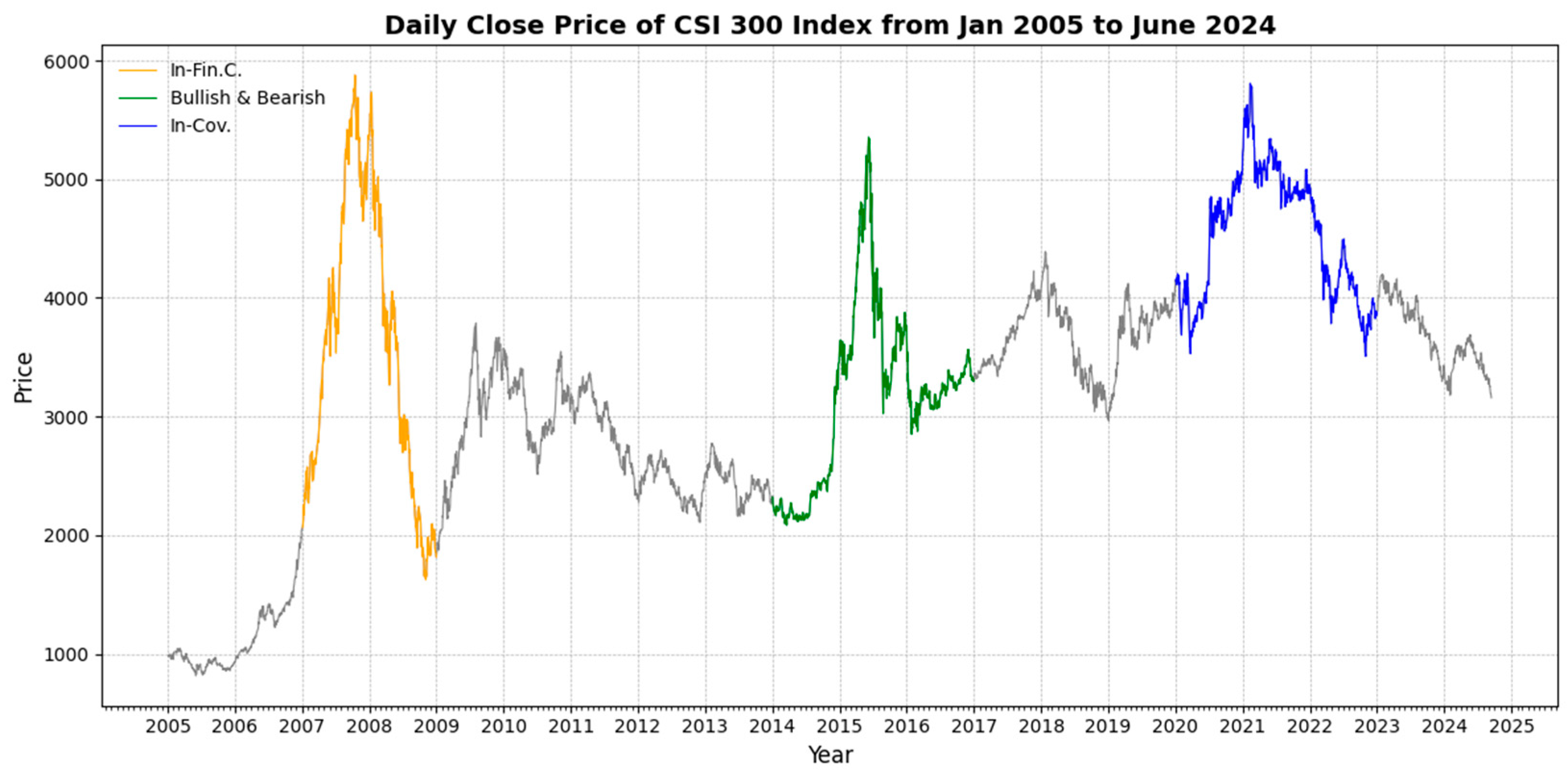
The dataset consists of daily stock data from the iFinD database, covering the period from 1 January 2005, to 28 June 2024, spanning 7118 days (233 months) and including a total of 5612 Chinese stocks. The cut-off at June 2024 corresponds to the timeframe available when the research was initiated. The chosen horizon already spans nearly two decades and covers three major market crises, providing a sufficiently comprehensive basis for the analysis.

The selection criteria and methodology used to construct the sample are consistent with the study of Do and Faff (2012). To minimize trading costs and avoid potential complications, this study further refines the sample to include only liquid stocks by excluding the bottom decile of stocks by market capitalization in each formation period. The formation period refers to the historical window during which stock pairs are identified and dependence structures are estimated, before strategies are implemented in the subsequent trading period.

In addition, stocks priced below RMB 1 (YUAN) during the formation period are excluded to avoid the influence of penny stocks, which typically suffer from poor liquidity, higher transaction costs, and greater susceptibility to speculative trading and price manipulation. To enhance robustness and better replicate real-world trading conditions, stocks that experience at least one non-trading day in any formation period within the corresponding trading period are also excluded. Overall, the data screening procedure ensures sample liquidity and consistency with prior literature (Do & Faff, 2012).

Also, the sample is well diversified across industries. Based on the Wind/CSMAR sector classification, the dataset covers all major sectors of the Chinese economy, with financials, industrials, and information technology jointly accounting for more than half of the firms, while consumer staples, energy, utilities, and healthcare also have meaningful representation. This broad sectoral distribution ensures that the analysis is not dominated by any single industry and captures heterogeneous trading behaviors across the market.

Furthermore, the sample period spans several important structural shifts in the Chinese equity market. These include the completion of the split-share reform in 2005, the introduction of stock index futures in 2010, the market turmoil and government interventions during the 2015 crash, and more recent institutional changes such as the adoption of the registration-based IPO system in 2019 and the increasing participation of northbound capital flows through the Stock Connect program after 2020. By covering nearly two decades and incorporating these diverse market regimes, the dataset provides a comprehensive setting to assess the robustness and stability of pairs trading strategies under varying structural and regulatory conditions.

4. Methodology

Pairs trading is a mean-reverting, contrarian investment strategy based on an assumed price relationship between two securities. This strategy involves taking long and short positions simultaneously—buying the undervalued security while short selling the overvalued one—to exploit short-term deviations from their expected relationship. Once the price relationship reverts to its mean, both positions are closed, allowing the investor to realize profits.

This study evaluates the performances of four distinct PTSs using data from the iFinD database, covering Chinese stocks from 2005 to 2024. For each strategy, a six-month trading period is employed, during which the strategy is executed based on parameters estimated over the preceding 12 months, referred to as the formation period. These strategies are implemented on a monthly basis without waiting for the current trading period to complete, resulting in six overlapping portfolios, with each portfolio corresponding to a trading period initiated in a different month. This rolling-window structure naturally separates model estimation and trading execution, ensuring that all reported strategy performance is evaluated out-of-sample.

In the DM outlined in Section 4.1, the benchmark strategy, potential security pairs are ranked based on the sum of squared deviations of their normalized prices during the formation period. Once the pairs are established, the spread between the two securities is monitored throughout the trading period. If the spread deviates beyond a predetermined threshold, this triggers the opening of simultaneous long and short positions. This strategy serves as the primary benchmark to assess the performance of the copula and mixed copula-based pairs trading strategies.

The copula-based strategy is specifically designed to enhance computational efficiency, making it practical for implementation by traders. This approach combines elements of the DM with the copula framework. Stock pairs are first ranked and selected based on the sum of squared deviations, after which a range of marginal and copula distributions are fitted to the selected pairs. Copulas are then employed (as detailed in Section 4.2) to model the dependence structure between the stocks in each pair and to detect deviations from their most likely relative pricing (Xie et al., 2016). To implement trading, two mispricing indices are defined to capture the relative overvaluation or undervaluation of the stocks within each pair, which serve as triggers for initiating long-short positions when prices deviate from their estimated fair values. Additionally, the analysis is extended by incorporating mixed copulas to further explore and refine the copula-based strategy.

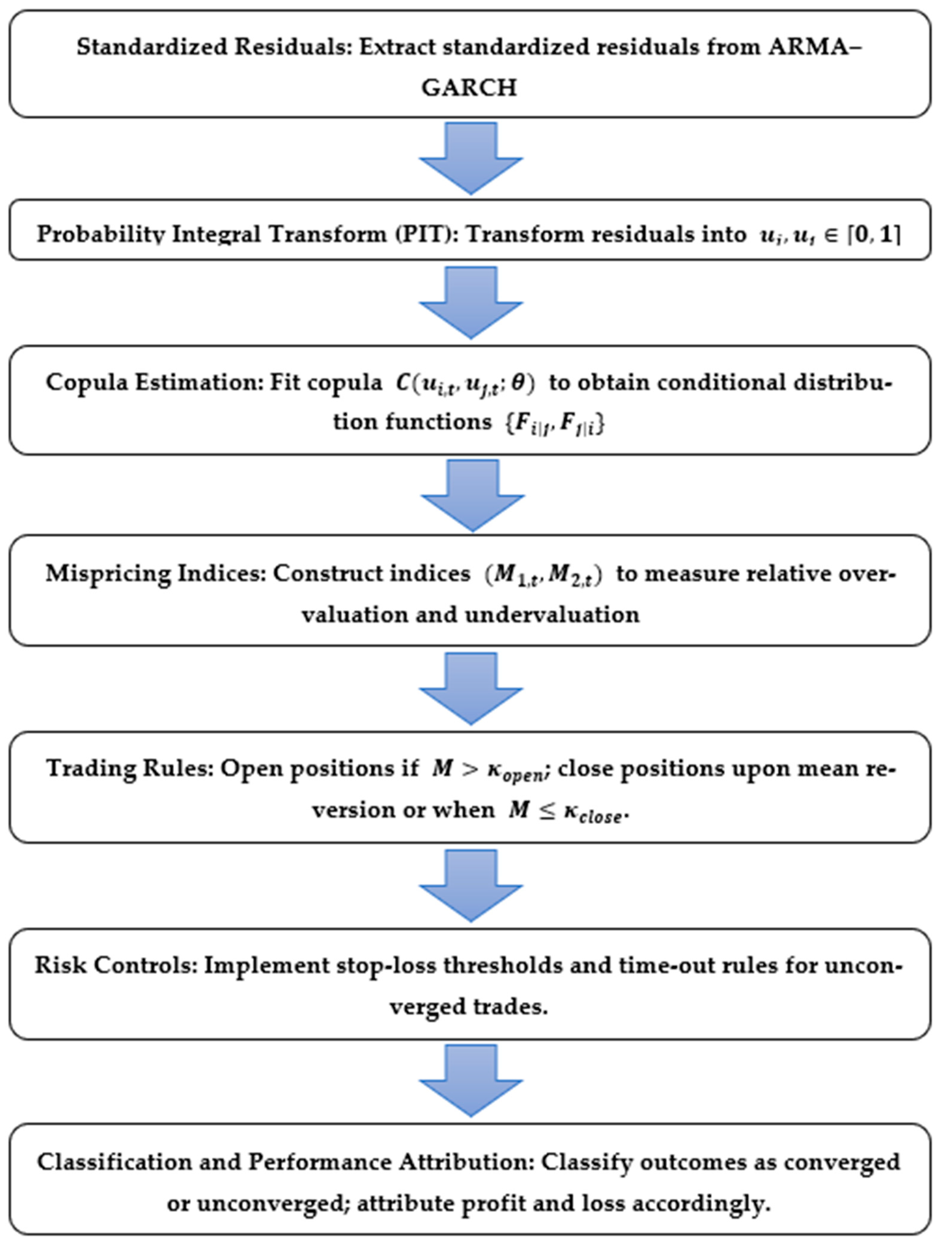
Before delving into the technical details, it is useful to provide an overview of the proposed framework. Figure 1 summarizes the two-step copula-based pairs trading strategy, from data preparation and pair selection to copula modeling, signal generation, and portfolio evaluation.

4.1. The Distance Method

In the DM, the spread between the normalized prices of all potential stock pairs is computed during a 12-month formation period. The normalized price is defined as a cumulative return index adjusted for dividends and corporate actions, with a base value of 1 RMB at the start of the formation window. Following Gatev et al. (2006), the Sum of Squared Deviations (SSD) of the spread is then calculated for each pair. The SSD statistic is the sum of squared deviations of normalized spreads over the formation period, and lower values indicate more stable and tightly co-moving spreads. This property makes SSD a natural criterion for identifying potentially profitable pairs in statistical arbitrage. The top N pairs with the lowest SSD are selected as the set of nominated pairs for trading in the subsequent 6-month trading period. In addition, the standard deviation of the spread during the formation period is recorded and used as a key threshold in trading decisions. A single stock can appear in multiple pairs, provided that the other stock differs.

At the start of each trading period, stock prices are rescaled to RMB 1, and spreads are recalculated and continuously monitored. A trade is opened whenever the spread deviates by two or more historical standard deviations (measured in the formation period): a long position is taken in the undervalued stock and a short position in the overvalued stock. Positions are closed once the spread converges back to zero, completing a round-trip trade, after which the pair remains eligible for subsequent trades within the same trading period. Since the entry threshold is fixed at two standard deviations, pairs with lower volatility require smaller absolute deviations to trigger trades, which may increase the risk of convergence failures. Time-varying transaction costs (see Section 4.5) further influence performance, and a detailed sensitivity analysis is provided in Section 5.

Building on this framework, Do and Faff (2012) propose the SSD-NZC selection method, which further filters pairs by incorporating the Number of Zero-Crossings (NZC). Specifically, SSD-NZC method is defined as the intersection of pairs in the first (lowest) SSD decile and the first (lowest) NZC decile, denoted as “Top N Pairs in 1st SSD Decile ∩ 1st NZC Decile”. The NZC metric counts how often the price spread crosses zero during the formation period, with more crossings implying more frequent mean reversion. Thus, SSD-NZC method selects pairs that not only have stable spreads but also exhibit a strong tendency to revert toward equilibrium, thereby reducing the likelihood of prolonged divergence.

Extending this idea, the SSD-Hurst selection method is introduced, which replaces NZC with the Hurst exponent as an alternative measure of mean-reversion strength. The Hurst exponent, originally developed in the context of long-memory processes, quantifies the persistence or anti-persistence of a time series. A value of H < 0.5 indicates anti-persistence, i.e., strong mean-reverting behavior, whereas H > 0.5 reflects persistence, i.e., trending behavior. In the SSD-Hurst approach, it is defined the portfolio as “Top N Pairs in 1st SSD Decile ∩ 1st Hurst Decile”. By selecting pairs that simultaneously rank in the lowest SSD decile (stable spreads) and the lowest Hurst decile (strongest mean reversion), SSD-Hurst method is designed to capture pairs that combine low deviation in spreads with the highest theoretical propensity for mean reversion.

4.2. The Mispricing Index Copula Method

4.2.1. Method Framework Overview

A copula is a mathematical function that links marginal distribution functions to form their joint distribution, thereby capturing the dependence structure among the marginal distributions. A copula function is defined as a multivariate joint distribution function with uniform marginal distributions:

$$C(u_1,u_2,\dots ,u_n)=P(U_1\le u_1,U_2\le u_2,\dots ,U_n\le u_n)$$

(1)

where $u_i\in \left[\mathrm{0,1}\right]$ for $i=\mathrm{1,2},\dots ,n$. Now consider a set of $n$ random variables $X_1,X_2,\dots ,X_n$ with continuous marginal distribution functions $F_1\left(x_1\right),F_2\left(x_2\right),\dots ,F_n\left(x_n\right)$. Since any random variable can be transformed into a uniform random variable by applying its cumulative distribution function (CDF), i.e., $U_i=F_i\left(X_i\right)$ where $U_i\sim Uniform\left(\mathrm{0,1}\right)$, the copula function of these random variables can be defined as follows:

$$F(x_1,x_2,\dots ,x_n)=C\left(F_1\right(x_1),F_2(x_2),\dots ,F_n(x_n\left)\right)$$

(2)

If the marginal distribution functions $F_i$ and the copula function $C$ are differentiable up to the first and $n-th$ order, respectively, the joint probability density function (pdf) can be expressed as the product of the marginal density functions and the copula density function $f\left(x_1,x_2,\dots ,x_n\right)=f_1\left(x_1\right)\times f_2\left(x_2\right)\times \dots \times f_n\left(x_n\right)\times c\left(F_1\right(x_1),F_2(x_2),\dots ,F_n(x_n\left)\right)$.

Where $c$ is the copula density function, obtained by differentiating the copula function $C$ with respect to each of its arguments:

$$c(u_1,u_2,\dots ,u_n)={\displaystyle \frac{{\partial }^{n}C(u_1,u_2,\dots ,u_n)}{\partial u_1\partial u_2\dots \partial u_n}}$$

(3)

Equation (3) allows the separation of a multivariate distribution into two components: the individual marginal density functions and the copula density function. This decomposition is crucial because the marginal density functions capture the characteristics of the individual distributions, while the copula density function represents the dependency structure between them. Consequently, all dependence properties between the random variables are encapsulated within the copula density function, making it an essential tool for modeling complex dependencies.

Therefore, copulas offer greater flexibility in modeling multivariate distributions by enabling the independent modeling of each marginal distribution without imposing assumptions on their joint behavior. Furthermore, the selection of the copula is independent of the choice of the marginal distributions, allowing for a more versatile approach to dependency modeling. Unlike traditional methods that often assume linear dependence structures between variables, copulas eliminate this constraint and provide a way to capture more complex dependency patterns. By choosing appropriate copula functions, a variety of dependence structures, including asymmetric dependencies, can be effectively modeled.

Let $X_1$ and $X_2$ be two random variables with respective marginal distribution functions $F_1\left(x_1\right)$ and $F_2\left(x_2\right)$a and the joint bivariate distribution function $F(X_1,X_2)$. Defining $U_1=F_1\left(X_1\right)$ and $U_2=F_2\left(X_2\right)$, where $U_1,U_2\sim Uniform\left(\mathrm{0,1}\right)$, the copula function linking these variables is given by $C(u_1,u_2)=P(U_1\le u_1,U_2\le u_2)$. By definition, the partial derivatives of the copula function yield the conditional distribution functions (Aas et al., 2009):

$$h_1(u_1\mid u_2)=P(U_1\le u_1\mid U_2=u_2)={\displaystyle \frac{\partial C(u_1,u_2)}{\partial u_2}}$$

(4)

$$h_1(u_2\mid u_1)=P(U_2\le u_2\mid U_1=u_1)={\displaystyle \frac{\partial C(u_1,u_2)}{\partial u_1}}$$

The conditional distribution functions $h_1$ and $h_2$ allow the estimation of the probability that one random variable is less than a given value, conditional on the other variable having a specific value. Applying these functions in a PTS enables the assessment of the probability that one stock in a pair increases or decreases relative to its current price, given the movement of the other stock.

Xie et al. (2016) utilize the property that the partial derivative of the copula function yields the conditional distribution function to propose a measure that quantifies the degree of mispricing. Let $R_t^X$ and $R_t^Y$ represent the random daily returns of stocks $X$ and $Y$ at time $t$ and $r_t^X$ and $r_t^Y$ denote their respective realized values at time $t$. The conditional probabilities can be defined as:

$${MI}_{X|Y}^t={\displaystyle \frac{\partial C(u_1,u_2)}{\partial u_2}}=P(R_t^X<r_t^X\mid R_t^Y=r_t^Y)$$

(5)

$${MI}_{Y|X}^t={\displaystyle \frac{\partial C(u_1,u_2)}{\partial u_1}}=P(R_t^X<r_t^X\mid R_t^Y=r_t^Y)$$

where $u_1=F_X\left(r_t^X\right)$ and $u_2=F_Y\left(r_t^Y\right)$.

Therefore, these conditional probabilities, ${MI}_{X|Y}^t$ and ${MI}_{Y|X}^t$, measure whether the return of stock $X$ is relatively high or low at time $t$, given the return of stock $Y$ at the same time and their historical relationship, and vice versa. If ${MI}_{X|Y}^t=0.5$, it indicates that the return $r_t^X$ is neither significantly high nor low relative to $r_t^Y$ based on their historical relationship, implying no mispricing. In other words, a conditional value of 0.5 suggests that stock $X$ is fairly priced compared to stock $Y$ on that day.

The above-mentioned conditional probabilities reflect relative mispricing for a single day only. To capture the overall degree of relative mispricing, two mispricing indices are defined $m_{1,t}$ and $m_{2,t}$ for stocks $X$ and $Y$ as $m_{1,t}={MI}_{X|Y}^t-0.5$ and $m_{2,t}={MI}_{Y|X}^t-0.5$. At the beginning of each trading period, two cumulative mispricing indices $M_{1,t}$ and $M_{2,t}$ are initialized to zero and then updated daily according to the following Equation (6):

$$M_{1,t}=M_{1,t-1}+m_{1,t}$$

(6)

$$M_{2,t}=M_{2,t-1}+m_{2,t}$$

for $t=1,\dots ,T$. By construction, $M_{1,t}$ and $M_{2,t}$ are non-stationary time series, and their properties depend on the correlation between $m_{i,t}$ and $M_{i,t-1}$. If the correlation is zero, $M_{i,t}$ follows a pure random walk, suggesting that statistical arbitrage opportunities are absent. A positive correlation indicates a tendency for $M_{i,t}$ to diverge, potentially resulting in losses. Conversely, a negative correlation suggests that $M_{i,t}$ tends to revert back to zero when it moves significantly away from the equilibrium, thereby generating profit opportunities. Empirically, $M_{i,t}$ may alternate between these behaviors, and as long as the mean-reverting mechanism dominates, the strategy can yield profitable outcomes.

This approach is particularly advantageous because it captures mispricings over multiple time periods, offering insights into how far the prices deviate from their equilibrium. Unlike single-day mispricing indices, cumulative mispricing indices lead to a more stable trading strategy. Positive (negative) values of $M_{1,t}$ and negative (positive) values of $M_{2,t}$ indicate that stock 1 (stock 2) is overvalued relative to stock 2 (stock 1). Figure 2 illustrates this process, showing how mispricing indices are translated into trading signals through opening and closing thresholds, and how these signals are executed as self-financing long–short positions under transaction cost considerations. Additionally, the analysis is extended by incorporating mixed copulas to further explore and refine the copula-based strategy.

4.2.2. Trading Strategy

Similarly to the DM, all potential stock pairs are ranked based on the SSD-Hurst method of their normalized prices during the formation period, and the top N pairs with the lowest SSD values are selected for trading in the subsequent trading period. For each of these selected pairs, the Inference for Margins (IFM) method (Joe, 1997) is employed to fit copula models. A range of copula types is considered, including Clayton, Frank, Gaussian, Gumbel, and Student-t copulas, with conditional probability functions given in

Table 1. Five Copula Conditional Probability Functions.

Copula	$P(U_1\le u_1\mid U_2=u_2)$
Student-t	$h(u1,u2;\rho ,\nu )=t_{\nu +1}({\displaystyle \frac{x_1-\rho x_2}{\sqrt{\frac{(\nu +x_2^2)(1-{\rho }^2)}{v+1}}}})$ $x_i=t_v^{-1}\left(u_i\right),u_i\in \left(0,1\right),i=1,2$	$\rho \in (-1,1)$ $v>0$
Clayton	$h(u_1,u_2;\theta )={u_2}^{-\left(\theta +1\right)}{({u_1}^{-\theta }+{u_2}^{-\theta }-1)}^{-{\displaystyle \frac{1}{\theta }}-1}$	$\theta >0$
Frank	$h(u_1\mid u_2;\theta )={\displaystyle \frac{\theta e^{-\theta u_1}}{e^{-\theta }+(e^{-\theta u_1}-1)(e^{-\theta u_2}-1)}}$ $C(u_1,u_2;\theta )=-{\displaystyle \frac{1}{\theta }}ln[1+{\displaystyle \frac{(e^{-\theta u_1}-1)(e^{-\theta u_2}-1)}{e^{-\theta }-1}}]$	$u_1,u_2\in (\mathrm{0,1})$ $\theta \in R$
Gumbel	$h(u_1,u_2;\theta )=C_{\theta }(u_1,u_2)\times {[{(-ln{u}_1)}^{\theta }+{(-ln{u}_2)}^{\theta }]}^{{\displaystyle \frac{1-\theta }{\theta }}}\times {(-ln{u}_2)}^{\theta -1}\times {\displaystyle \frac{1}{u_2}}$ $C_{\theta }\left(u_1,u_2\right)=\mathrm{e}\mathrm{x}\mathrm{p}(-{[{(-ln{u}_1)}^{\theta }+{(-ln{u}_2)}^{\theta }]}^{{\displaystyle \frac{1}{\theta }}})$	$\theta >0$
Gaussian	$h(u_1\mid u_2;\rho )=\Phi ({\displaystyle \frac{{\Phi }^{-1}(u_1)-\rho {\Phi }^{-1}(u_2)}{\sqrt{1-{\rho }^2}}})$	$\rho \in (-1,1)$

Note: This table shows five conditional probability functions of copulas used in the copula method.

.

These five single copula families are selected because they capture distinct forms of dependence widely discussed in the financial econometrics’ literature. Clayton and Gumbel emphasize lower- and upper-tail dependence, respectively; Frank represents a symmetric, non-tail-dependent structure; Student-t accounts for heavy-tailed dependence; and Gaussian reflects linear correlation. The purpose of including this diverse set is not to favor one particular specification, but rather to compare how different dependence structures influence the performance of pairs trading strategies.

In addition to single-family copulas, this study also considers several mixed copulas (e.g., CFG, CJF, CJG, and FJG). The rationale for including these mixtures is that individual copulas typically capture only one type of dependence structure—such as lower-tail, upper-tail, or symmetric dependence—whereas mixed copulas combine multiple families to account for heterogeneous features simultaneously. For example, combinations like Clayton–Gumbel can jointly capture both lower- and upper-tail dependence, while Clayton–Frank–Gaussian mixtures provide more flexibility in modeling intermediate and symmetric dependencies. The inclusion of mixed copulas therefore enhances the robustness of the comparison by allowing for more realistic and flexible dependence structures that are frequently observed in financial markets.

Rather than selecting the optimal copula by maximizing the log-likelihood of each copula density function and evaluating its fit using the Akaike Information Criterion (AIC) and Bayesian Information Criterion (BIC), the returns generated by each of the five copula models are computed and analyzed individually. Similarly to Rad et al. (2016), the following steps are proposed to obtain $M_{1,t}$ and $M_{2,t}$ using copula-based models.

First, the daily returns for each stock during the formation period are calculated, and the marginal distributions of these returns are estimated by fitting an appropriate ARMA (p, q)-GARCH (r, s) model to each univariate time series.

Following Liew and Wu (2013), Rad et al. (2016), and Stübinger et al. (2018), the marginal distributions are modeled using ARMA–GARCH process. This specification represents the standard approach in the copula–pairs trading literature, as it effectively captures volatility clustering and conditional heteroskedasticity in financial returns while remaining computationally tractable for large-scale applications.

Although alternative specifications such as EGARCH, TGARCH, Markov-switching GARCH, or Generalized Autoregressive Score (GAS) models can offer additional flexibility, prior studies have consistently shown that these variants mainly refine volatility dynamics without materially altering the dependence structure captured by the copula. For instance, Patton (2006) demonstrates in exchange rate markets that copula-based estimates of asymmetric dependence remain robust under different GARCH-type marginals. Similarly, Jondeau and Rockinger (2006) show in international stock markets that switching from standard GARCH to more flexible forms such as EGARCH or TGARCH improves marginal volatility fit but leaves copula dependence estimates largely unchanged. Rodriguez (2007) further finds that even when accounting for structural breaks and heteroskedasticity in financial contagion settings, the tail dependence captured by copulas remains stable. More recently, Oh and Patton (2017) highlight in a high-dimensional context that the copula framework provides consistent dependence estimates regardless of marginal specifications, while Chen et al. (2021) propose a semi-nonparametric GARCH-filtered copula estimator that underscores the practical feasibility of separating marginals from the copula dependence structure. In a large-scale forecasting exercise, Fritzsch et al. (2024) further document that model risk in multivariate risk prediction is driven predominantly by the choice of copula rather than the marginal distribution. Taken together, these studies confirm that while advanced volatility models may refine marginal dynamics, the copula-based dependence structure—particularly tail dependence and rank correlation—remains largely stable. Consequently, the choice of ARMA–GARCH, though simpler, does not materially bias the copula estimates, making it a widely accepted and computationally practical option in the literature.

The adoption of ARMA–GARCH is therefore motivated by a balance between methodological adequacy and computational feasibility, especially given the scope of this study, which covers more than 5000 stocks over nearly two decades. The focus here is on evaluating the relative profitability of alternative pairs trading strategies rather than on conducting a comprehensive comparison of marginal models.

That said, a limitation of this choice is that ARMA–GARCH assumes stable dynamics within regimes and may inadequately capture abrupt structural breaks, leverage effects, or regime switches, particularly during periods of extreme market turbulence. While this is consistent with common practice in the literature, future research could fruitfully explore the incorporation of regime-switching, smooth-transition, or score-driven models to assess whether the results remain robust under more complex marginal specifications.

This process yields the estimated conditional mean ${\widehat{u}}_{i,t}$ and conditional standard deviation ${\widehat{\sigma }}_{i,t}$ for each stock $i$. Using these estimated parameters, the standardized residuals are then constructed for each asset $i=1,\dots ,N$ and each time $t=1,\dots ,T$, where $N$ represents the number of assets and $T$ denotes the length of the time series, as follows:

$${\widehat{\epsilon }}_{i,t}={\displaystyle \frac{r_{i,t}-{\widehat{u}}_{i,t}}{{\widehat{\sigma }}_{i,t}}}$$

(7)

where $r_{i,t}$ is the $t-th$ return of asset $i$. Next, the standardized residuals are transformed into pseudo-observations defined as $u_{i,t}={\displaystyle \frac{T}{T+1}}{F}_{i,t}({\widehat{\epsilon }}_{i,t})$, where $F_{i,t}$ is the empirical distribution function of the standardized residuals for asset $i$.

Second, after estimating the marginal distributions in the previous step, a two-dimensional copula model is fitted to the data transformed into [0, 1] margins in order to link the joint distribution to the marginals ${\widehat{F}}_{i,t}$ and ${\widehat{F}}_{j,t}$. Specifically, the joint CDF is defined as:

$$\widehat{H}(r_{i,t},r_{j,t})=C\left({\widehat{F}}_{i,t}\right({\widehat{\epsilon }}_{i,t}),{\widehat{F}}_{j,t}({\widehat{\epsilon }}_{j,t}\left)\right)$$

(8)

where $\widehat{H}$ represents the estimated joint CDF and $C$ denotes the copula function. In this step, several copulas are evaluated, including the Gaussian (Normal), Student-t (T) (elliptical copulas), and a variety of Archimedean copulas such as the Clayton, Frank, and Gumbel copulas.

Third, to measure the degree of mispricing, the conditional probabilities are computed as ${MI}_{X|Y}$ and ${MI}_{Y|X}$ for each day during the trading period by taking the first derivative of the copula function using the estimated parameters.

Forth, long and short positions in stocks $Y$ and $X$ are established on days when $M_{1,t}>{∆}_1$ and $M_{2,t}<{∆}_2$, provided there are no existing positions in either $X$ or $Y$. Similarly, positions are established in $X$ and $Y$ when $M_{1,t}<{∆}_2$ and $M_{2,t}>{∆}_1$, if no positions are currently held.

Fifth, all open positions are closed once $M_{1,t}$ reaches ${∆}_3$ or $M_{2,t}$ reaches ${∆}_4$, where ${∆}_1$, ${∆}_2$, ${∆}_3$ and ${∆}_4$ are predetermined thresholds. If these thresholds are not met, the positions are automatically closed on the final day of the trading period. Practitioners can freely select these threshold values. However, instead of choosing arbitrary values, the trading thresholds are set to generate a comparable number of trading signals, specifically focusing on the top N pairs in this study. This approach ensures a fair comparison of the performance across different strategies. For the analysis, following prior studies (e.g., Xie et al., 2016; Rad et al., 2016), the thresholds are set as ${∆}_1=0.6$, ${∆}_2=-0.6$, and ${∆}_3={∆}_4=0$.

4.3. The Optimal Copula Method

4.3.1. Method Framework Overview

Building on the MPI copula method described in Section 4.2, the optimal copula method seeks to enhance the modeling of dependency structures between stock pairs by selecting the most appropriate copula function for each pair individually. While the MPI copula method considers several predefined copulas and analyzes their returns separately, the optimal copula method systematically evaluates multiple copula models for each stock pair and selects the one that best fits the data based on a statistical criterion. This tailored approach allows for a more precise capture of the dependence structures inherent in each stock pair, potentially leading to improved trading performance.

The core idea of the optimal copula method is to fit a range of copula models to the historical data of each selected stock pair during the formation period and choose the copula that minimizes the Schwarz Information Criterion (SIC), also known as the BIC. The SIC penalizes model complexity while rewarding goodness of fit, thus balancing overfitting and underfitting. By selecting the copula with the lowest SIC, the chosen model is selected to provide the best trade-off between model simplicity and explanatory power for the dependence structure between the stock pair.

4.3.2. Trading Strategy

Similarly to the DM, all potential stock pairs are ranked based on the SSD-NZC method of their normalized prices during the formation period, and the top N pairs with the lowest SSD values are selected for trading in the subsequent trading period. For each of these selected pairs, the IFM method (Joe, 1997) is employed to fit copula models. Multiple copula models are then fitted using the return data from the formation period, including Clayton, Frank, Gumbel, Gaussian, and Student-t copulas.

The fitting process begins with data preparation, where the log returns of each stock are calculated and aligned to ensure that the return series cover the same time periods without missing values. Following this, the marginal distributions of the returns are estimated by fitting appropriate models, such as ARMA-GARCH, and standardized residuals are computed. After the standardized residuals are available, they are transformed into pseudo-observations within the [0, 1] interval using their empirical CDFs. The next step involves fitting different copula models to these pseudo-observations and calculating the SIC for each model. The SIC is calculated using the formula $SIC=-2\times ln\left(L\right)+k\times ln\left(T\right)$, where L represents the likelihood of the copula model, k is the number of parameters in the model, and T is the number of observations. The final step is selecting the copula model with the lowest SIC value for each stock pair. This copula is considered the optimal model for capturing the dependence structure between the two stocks.

With the optimal copula models selected for each stock pair, the trading strategy is implemented during the trading period through several key steps. First, stock prices for both the formation and trading periods are standardized by subtracting the mean and dividing by the standard deviation calculated during the formation period. This standardization ensures consistent scaling of the data across different periods.

Next, the empirical CDFs of the standardized returns from the formation period are used to transform the standardized returns from the trading period into pseudo-observations. This transformation maintains the dependency structure learned during the formation period.

For each day in the trading period, mispricing indices are computed by calculating the conditional probabilities using the derivative of the optimal copula function with respect to each margin. The cumulative mispricing indices $M_{1,t}$ and $M_{2,t}$ are initialized to zero at the start of the trading period. These indices are updated daily by adding the mispricing indices minus 0.5, thus aggregating mispricing signals over time. These cumulative indices serve as the basis for trading decisions.

When the cumulative mispricing indices cross predetermined thresholds, trading signals are generated. If $M_{1,t}$ exceeds threshold ${∆}_1$ and $M_{2,t}$ is below ${∆}_2$, a long-short position is opened in stocks Y and X. Conversely, positions are opened when $M_{1,t}$ is below ${∆}_2$ and $M_{2,t}$ exceeds ${∆}_1$, provided no positions are currently held. Positions are closed either when $M_{1,t}$ reaches ${∆}_3$ or $M_{2,t}$ reaches ${∆}_4$, or at the end of the trading period if no thresholds are met. In this implementation, following prior studies (e.g., Xie et al., 2016; Rad et al., 2016), these thresholds are set to ${∆}_1=0.6$, ${∆}_2=-0.6$, and ${∆}_3={∆}_4=0$.

4.4. The Mixed Copula Method

4.4.1. Method Framework Overview

In the previous sections, individual copula models were explored to capture the dependence structure between stock pairs in pairs trading strategies. While selecting the optimal copula for each stock pair enhances the modeling of dependencies, it may still fall short in capturing the complex and diverse dependency patterns that can exist in financial markets. To address this limitation, the Mixed Copula Method is introduced, which employs a mixture of multiple copulas to model the dependence structure more flexibly and accurately.

A mixed copula combines several copula functions, each weighted by a coefficient that reflects its contribution to the overall dependence structure. This approach allows the capture of different aspects of dependency, such as tail dependence and asymmetry, by blending the strengths of various copula models. The flexibility of mixed copulas makes them particularly suitable for modeling the intricate relationships between asset returns, which may not be adequately represented by a single copula.

A mixture of d component copulas is defined as follows:

$$C(u_1,u_2)\in C_M=\{{\sum }_{i=1}^d{\omega }_i{C}_i(u_1,u_2)\hspace{0.17em}\mid \hspace{0.17em}{\sum }_{i=1}^d{\omega }_i=1,\hspace{0.17em}{\omega }_i\ge 0,\hspace{0.17em}i=1,\dots ,d\}$$

(9)

where $C(u_1,u_2)$ is the mixed copula function, $C_M$ represents the set of all possible mixed copulas formed by the convex combination of d copula functions, $C_i(u_1,u_2)$ denotes the $i-th$ copula function in the mixture, and ${\omega }_i$ is the weight assigned to the $i-th$ copula, satisfying ${\omega }_i\ge 0$ and $\sum _{i=1}^d{\omega }_i=1$.

This framework allows the construction of flexible mixed copula models with varying numbers of components, such as two, three, or four copulas. By adjusting the weights ${\omega }_i$ and selecting appropriate copula functions $C_i$, the mixed copula can be tailored to capture the specific dependency characteristics of each stock pair.

Based on the empirical results, four flexible mixed copula models are constructed. These four copula models are defined as follows:

The mixture of Clayton, Frank, and Gumbel copulas:

$$C_{CFG}(u_1,u_2)={\omega }_1{C}_{\alpha }^C(u_1,u_2)+{\omega }_2{C}_{\beta }^F(u_1,u_2)+(1-{\omega }_1-{\omega }_2)C_{\delta }^G(u_1,u_2)$$

(10)

The mixture of Frank, Gumbel, and Student-t copulas:

$$C_{FJG}(u_1,u_2)={\omega }_1{C}_{\alpha }^F(u_1,u_2)+{\omega }_2{C}_{\beta }^J(u_1,u_2)+(1-{\omega }_1-{\omega }_2)C_{\delta }^G(u_1,u_2)$$

(11)

The mixture of Clayton, Student-t, and Gumbel copulas:

$$C_{CJG}(u_1,u_2)={\omega }_1{C}_{\alpha }^C(u_1,u_2)+{\omega }_2{C}_{\beta }^J(u_1,u_2)+(1-{\omega }_1-{\omega }_2)C_{\delta }^G(u_1,u_2)$$

(12)

The mixture of Clayton, Student-t, and Frank copulas:

$$C_{CJF}(u_1,u_2)={\omega }_1{C}_{\alpha }^C(u_1,u_2)+{\omega }_2{C}_{\beta }^J(u_1,u_2)+(1-{\omega }_1-{\omega }_2)C_{\delta }^F(u_1,u_2)$$

(13)

In these formulations, $C_{\alpha }^C$, $C_{\beta }^F$, $C_{\delta }^G$, and $C_{\beta }^J$ represent the Clayton, Frank, Gumbel, and Joe copulas with parameters α, β, and δ, respectively. ${\omega }_1$ and ${\omega }_2$ are the weights assigned to the first and second copulas in the mixture, with $(1-{\omega }_1-{\omega }_2)$ being the weight of the third copula.

4.4.2. Estimation of Mixed Copula Parameters

To estimate the parameters α, β, and δ, and the weights ω_i of the mixed copula models, a penalized maximum likelihood estimation method from Cai and Wang (2014) is employed. Specifically, the negative log-likelihood function augmented with a penalty term that encourages sparsity in the weights is minimized. The objective function to be minimized is:

$${\mathcal{L}}_p(\theta ,\omega )=-{\sum }_{t=1}^{T}ln({\sum }_{i=1}^d{\omega }_i{C}_i(u_{1,t},u_{2,t}))+\lambda {\sum }_{i=1}^d{P}_{\gamma }\left({\omega }_i\right)$$

(14)

where T is the number of observations, $C_i(u_{1,t},u_{2,t})$ is the density function of the $i-th$ copula evaluated at $(u_{1,t},u_{2,t})$, and λ is a tuning parameter controlling the strength of the penalty. $P_{\gamma }\left({\omega }_i\right)$ is a penalty function, such as the smoothly clipped absolute deviation (SCAD) penalty, with parameter γ.

The inclusion of the penalty term serves to regularize the weights ${\omega }_i$, potentially setting some weights to zero and thus selecting a subset of copulas that best explain the dependency structure. This approach helps to prevent overfitting and reduces model complexity.

The estimation process begins with transforming the marginal distributions of the stock returns into uniform distributions on the interval [0, 1] using their empirical CDFs. This transformation produces the pseudo-observations $u_{1,t}$ and $u_{2,t}$, which serve as inputs for the copula modeling. The next step is to initialize the copula parameters α, β, and δ, as well as the weights ${\omega }_i$. These initial guesses provide a starting point for the iterative procedure. An Expectation-Maximization (EM) algorithm is then employed to refine these estimates. During the Expectation step, the current copula parameters are used to update the weights ${\omega }_i$ by calculating the expected log-likelihood. In the Maximization step, these updated weights are then used to maximize the penalized log-likelihood function with respect to the copula parameters α, β, and δ.

This EM process is repeated iteratively, and the convergence of the algorithm is monitored by checking whether the change in the estimated parameters falls below a predefined threshold. Alternatively, the algorithm halts once a maximum number of iterations is reached. The EM algorithm is particularly well-suited to this estimation problem, as it efficiently handles latent variables (in this case, the component memberships implied by the weights) and is robust in estimating mixture models.

4.5. Transaction Costs

Transaction costs are a critical factor in determining the profitability of PTS. Each full execution of a pairs trade involves two round-trip transactions, and the associated costs also include implicit market impact and potential short-selling fees. Given their cumulative effect, transaction costs can substantially reduce overall profitability when properly accounted for.

Given the complexity of estimating transaction costs in China after 2005, the best available proxy data representative of typical investors is employed. Since few studies document Chinese stock trading costs in detail, the primary data sources are disclosures from securities firms and the China Securities Regulatory Commission (CSRC), complemented by estimates from prior literature. For example, Pesaran and Timmermann (1995) set the cost of a round-trip trade for individual stocks at 0.5%, equivalent to 1% per round-trip pair trade. Bowen and Hutchinson (2016) report round-trip costs for paired trades of 71–73 bps, with an effective spread of 35–36 bps, while Zhang (2018), using data from the Cathay Securities database, estimates average transaction costs at approximately 70 bps. These external benchmarks provide context and support for the assumptions applied in this study.

In this study, a time-varying transaction cost dataset consistent with Do and Faff (2012) and Rad et al. (2016) is utilized. The rationale for this approach is that commissions and stamp duty represent the primary component of transaction costs, and these fees have undergone considerable changes over the past 20 years, which is the time span of the sample.

Using a constant commission rate could lead to inaccurate results; therefore, the institutional commission rates calculated by Do and Faff (2012) are adopted, starting at 40 basis points (bps) in 2005 and gradually decreasing to 15 bps in recent years for both buy and sell.

Following their methodology, for the Chinese stock market, the study period is further divided into two sub-periods with different market impact estimates: 40 bps for the period from 2005 to 2016 and 15 bps for the period from 2016 onward. Additionally, as the sample excludes stocks with low value and low market capitalization, it is assumed that the remaining stocks are relatively less expensive to short, and therefore, short selling costs are not explicitly included in the analysis. To ensure accuracy, market impact and slippage at 30 bps for both buy and sell are also considered.

For transparency, Appendix A 

Table A3. Overview of Trading Costs in the Chinese Stock Market.

Period	Commission	Stamp Duty	Market Impact and Slippage	Do and Faff (2012)	Zhang (2018)
Pre-Fin.C.: Jan 2005–Dec 2006	Ranged 0.1–0.3%. Selection criterion: 0.2% (buy and sell).	24 January 2005: Stamp duty reduced from 0.2 to 0.1%, applied to both buying and selling. Selection criterion: 0.2% (buy and sell)	Refer Do and Faff (2012) Assign a market impact cost of 0.3%.	1963–2009: commission + market impact of 0.60% (i.e., 0.34% + 0.26%) (60 bps).	SHSE 2005: 0.62% SZSE 2005: 0.73% SHSE 2006: 0.79% SZSE 2006: 0.82%
In-Fin.C.: Jan 2007–Dec 2008	Remained 0.1–0.3%. Selection criterion: 0.2% (buy and sell).	30 May 2007: Stamp duty increased from 0.1 to 0.3% (buys and sells). 24 April 2008: Reduced to 0.1%. 19 September 2008: applied to sales only at 0.1%. Selection criterion: 0.2% (buy and sell).	Based on historical experience, the slippage is set to a fixed value of 0.3%.	-	SHSE 2007: 0.92% SZSE 2007: 1.01% SSE 2008: 0.86% SZSE 2008: 0.87%
Post-Fin.C.: Jan 2009–Dec 2010	Ranged 0.05–0.2%. Selection criterion: 0.2% (buy and sell).	Maintained at 0.1%, sales only. Selection criterion: 0.1% (buy and sell).	-	-	SHSE 2009: 0.78% SZSE 2009: 0.81% SSE 2010: 0.68% SZSE 2010: 0.75%
Pre-B.N.B.: Jan 2011–Dec 2013	Ranged 0.05–0.1%. Selection criterion: 0.2% (buy and sell).	Maintained at 0.1%, sales only. Selection criterion: 0.1% (buy and sell).	-	-	SHSE 2011: 0.56% SZSE 2011: 0.60% SSE 2012: 0.52% SZSE 2012: 0.61%
In-Bullish: Jan 2014–May 2015	Remained 0.05–0.1%. Selection criterion: 0.2% (buy and sell).	Maintained at 0.1%, sales only. Selection criterion: 0.1% (buy and sell).	-	-	SHSE 2013: 0.64% SZSE 2013: 0.74% SSE 2014: 0.65% SZSE 2014: 0.73%
In-Bearish: June 2015–Dec 2016	Remained 0.05–0.1%. Selection criterion: 0.2% (buy and sell).	Maintained at 0.1%, sales only. Selection criterion: 0.1% (buy and sell).	-	-	SHSE 2015: 0.95% SZSE 2015: 0.93% SHSE 2016: 0.62% SZSE 2016: 0.68%
Pre-Cov.: Jan 2017–Dec 2019	Mostly 0.02–0.05%. Selection criterion: 0.05% (buy and sell).	Continued at 0.1%, sales only. Selection criterion: 0.1% (buy and sell).	-	-	-
In-Cov.: Jan 2020–Dec 2022	Around 0.02–0.03%. Selection criterion: 0.05% (buy and sell).	Maintained at 0.1%. Selection criterion: 0.1% (buy and sell).	-	-	-
Post-Cov.: Jan 2023–Jun 2024	Expected 0.02–0.03%. Selection criterion: 0.05% (buy and sell).	Expected to remain at 0.1%. Selection criterion: 0.1% (buy and sell).	-	-	-

Note: Regarding commission fees, since professional investors typically obtain the lowest available rates in actual trading, the lowest threshold is applied in the analysis to closely reflect real transaction costs. The data is based on information published by various brokerage firms. Regarding market impact, the conclusion of Do and Faff (2012) is referenced, and combined with the data obtained by Zhang (2018) from the official database, 60 bps is considered a reasonable estimate for both trades.

provides a detailed breakdown of transaction cost assumptions across different subperiods, including commissions, stamp duties, and market impact estimates, together with supporting references.

4.6. Return Calculation

The performances of the four pairs trading PTSs are recorded and evaluated using various performance metrics, including different measures of returns. Following the methodology of Gatev et al. (2006) and Do and Faff (2010), two types of returns are calculated: Return on Employed Capital and Return on Committed Capital.

Return on Employed Capital ($R_{EC}^m$) for month m is defined as the sum of the marked-to-market returns of all pairs traded in that month, divided by the number of pairs actively traded during the period. This metric reflects the actual returns generated by the capital that was employed in trades.

$$R_{EC}^m={\displaystyle \frac{\sum _{i=1}^n{r}_i}{n}}$$

(15)

where n is the number of traded pairs.

Return on Committed Capital ($R_{CC}^m$) for month m is calculated as the sum of the marked-to-market returns of all traded pairs, divided by the number of pairs that were allocated for trading (in the case of this paper, N pairs), regardless of whether they were traded or not. This measure is more conservative and reflects the opportunity cost associated with the capital set aside for trading, making it more suitable for reporting returns from a hedge fund perspective.

$$R_{CC}^m={\displaystyle \frac{\sum _{i=1}^n{r}_i}{N}}$$

(16)

The strategies are executed on a monthly basis without waiting for the completion of the current trading period, leading to the formation of six overlapping “portfolios” each month. The monthly excess return of a strategy is calculated as the equally weighted average return of these six portfolios. Given that trades do not always start at the beginning of the trading period or close exactly at the end, the full capital may not always be fully utilized. Additionally, some months may experience no trading activity. As idle capital does not accrue interest, the reported performance may be underestimated.

For both the DM and the copula-based method, positions are constructed as RMB 1 long–short positions. A RMB 1 long–short position is defined as simultaneously opening a RMB 1 long position and a RMB 1 short position. Since the proceeds from shorting one stock can be used to fund the purchase of the other stock, these positions are effectively self-financing and do not require additional capital. However, for the sake of return calculations, the standard convention of considering the total value of each long–short position as RMB 1 is adopted.

5. Results

5.1. Profitability of the Strategies

Table 2. Pairs Trading Strategies with Various Copulas Monthly Excess Returns before Transaction Costs.

Strategy	Mean	t-Stat	Std. Dev.	Sharpe	z-Stat	Skewness	Kurtosis	VaR (95%)	CvaR (95%)	JB Test (p-Value)
Panel A: Return on employed capital
SSD-Hurst	0.0084	2.26 **	0.0399	0.21	2.25 **	10.1033	120.5140	−0.0090	−0.0207	0
SSD-NZC	0.0082	2.44 **	0.0408	0.20	2.43 **	9.0968	106.0665	−0.0174	−0.0336	0
Clayton	0.0024	2.61 ***	0.0143	0.17	2.60 ***	−0.4138	2.9655	−0.0214	−0.0344	0
Frank	0.0026	3.03 ***	0.0128	0.21	3.02 ***	0.5756	6.8005	−0.0150	−0.0272	0
Gaussian	0.0030	3.63 ***	0.0129	0.23	3.62 ***	−0.1911	1.1780	−0.0180	−0.0258	0
Gumbel	0.0021	2.90 ***	0.0129	0.16	2.90 ***	−0.4994	1.3553	−0.0213	−0.0296	0
Student-t	0.0028	3.41 ***	0.0146	0.19	3.42 ***	−0.5746	2.2493	−0.0220	−0.0357	0
Optimal	0.0019	2.33 **	0.0116	0.16	2.32 **	−0.9099	3.2471	−0.0174	−0.0273	0
CFG	0.0020	2.33 **	0.0114	0.17	2.32 **	−0.4443	0.8605	−0.0181	−0.0257	0
CJF	0.0023	2.79 ***	0.0125	0.19	2.78 ***	−0.4243	2.6056	−0.0183	−0.0279	0
CJG	0.0023	2.82 ***	0.0127	0.18	2.82 ***	−0.2754	1.6407	−0.0218	−0.0290	0
FJG	0.0025	3.07 ***	0.0124	0.20	3.06 ***	−0.3048	2.1104	−0.0150	−0.0263	0
Panel B: Return on committed capital
SSD-Hurst	0.0082	2.21 **	0.0395	0.21	2.20 **	10.1453	121.1081	−0.0088	−0.0204	0
SSD-NZC	0.0081	2.39 **	0.0407	0.20	2.38 **	9.1478	106.8560	−0.0174	−0.0335	0
Clayton	0.0015	3.10 ***	0.0068	0.21	3.09 ***	−0.6681	3.5863	−0.0099	−0.0160	0
Frank	0.0021	4.32 ***	0.0068	0.30	4.31 ***	−0.8892	3.2254	−0.0086	−0.0146	0
Gaussian	0.0023	4.81 ***	0.0072	0.32	4.80 ***	−0.3102	1.5599	−0.0097	−0.0145	0
Gumbel	0.0017	4.04 ***	0.0072	0.24	4.04 ***	−0.4528	1.8285	−0.0110	−0.0155	0
Student-t	0.0018	4.37 ***	0.0073	0.25	4.37 ***	−0.8609	2.7959	−0.0110	−0.0178	0
Optimal	0.0016	3.62 ***	0.0062	0.26	3.61 ***	−0.9754	4.4947	−0.0087	−0.0125	0
CFG	0.0016	3.37 ***	0.0067	0.24	3.36 ***	−0.5552	1.8233	−0.0105	−0.0146	0
CJF	0.0019	4.17 ***	0.0067	0.28	4.16 ***	−0.3788	1.6577	−0.0085	−0.0136	0
CJG	0.0017	3.86 ***	0.0065	0.26	3.85 ***	−0.3094	1.3252	−0.0100	−0.0137	0
FJG	0.0021	4.43 ***	0.0072	0.29	4.42 ***	−0.7207	2.6422	−0.0095	−0.0158	0

Note: This table reports key distribution statistics for the monthly excess returns of various pairs trading strategies using different copulas before trading costs. The results are divided into two panels: Panel A represents returns on employed capital, and Panel B represents returns on committed capital. The time span covered in this study is from 2005 to 2024. The ‘JB test’ (Jarque–Bera test) results indicate non-normality for all strategies, as denoted by a p-value of 0. The column titled ‘t-stat’ provides the test statistic for the mean return estimate, calculated using Newey–West standard errors with six lags. The ‘z-stat’ column shows the test statistic for the Sharpe ratio estimate, based on Lo’s (2002) robust standard errors, which account for non-independence and non-identically distributed return time series. *** significant at the 1% level. ** significant at the 5% level.

and

Table 3. Pairs Trading Strategies with Various Copulas Monthly Excess Returns after Transaction Costs.

Strategy	Mean	t-Stat	Std. Dev.	Sharpe	z-Stat	Skewness	Kurtosis	VaR (95%)	CvaR (95%)	JB Test (p-Value)
Panel A: Return on employed capital
SSD-Hurst	0.0081	2.16 **	0.0397	0.20	2.15 **	10.2231	122.1875	−0.0095	−0.0199	0
SSD-NZC	0.0077	2.29 **	0.0407	0.19	2.28 **	9.1010	106.1485	−0.0179	−0.0342	0
Clayton	0.0011	1.33	0.0138	0.08	1.32	−0.4373	2.8047	−0.0223	−0.0342	0
Frank	0.0016	1.84 *	0.0125	0.12	1.83 *	0.4745	6.3886	−0.0158	−0.0278	0
Gaussian	0.0019	2.37 **	0.0126	0.15	2.36 **	−0.1816	0.9517	−0.0193	−0.0264	0
Gumbel	0.0008	1.14	0.0126	0.07	1.14	−0.5245	1.2660	−0.0219	−0.0300	0
Student-t	0.0023	2.69 ***	0.0125	0.18	2.68 ***	−0.1109	0.4397	−0.0193	−0.0249	0
Optimal	0.0009	1.20	0.0113	0.08	1.19	−0.8492	2.7027	−0.0171	−0.0272	0
CFG	0.0009	1.08	0.0111	0.08	1.08	−0.5046	0.8898	−0.0188	−0.0261	0
CJF	0.0013	1.55	0.0122	0.10	1.54	−0.4444	2.4726	−0.0191	−0.0281	0
CJG	0.0012	1.50	0.0124	0.10	1.49	−0.2420	1.5668	−0.0222	−0.0291	0
FJG	0.0015	1.82 *	0.0120	0.12	1.82 *	−0.4066	1.9814	−0.0164	−0.0269	0
Panel B: Return on committed capital
SSD-Hurst	0.0078	2.10 **	0.0395	0.20	2.09 **	10.1688	121.4783	−0.0092	−0.0208	0
SSD-NZC	0.0075	2.24 **	0.0407	0.18	2.23 **	9.1522	106.9420	−0.0178	−0.0341	0
Clayton	0.0007	1.41	0.0069	0.10	1.41	−0.7092	3.5148	−0.0110	−0.0169	0
Frank	0.0012	2.52 **	0.0069	0.18	2.51 **	−0.9186	3.2798	−0.0096	−0.0156	0
Gaussian	0.0015	3.09 ***	0.0072	0.21	3.09 ***	−0.3482	1.5314	−0.0105	−0.0154	0
Gumbel	0.0008	1.80 *	0.0072	0.11	1.80 *	−0.5171	1.8396	−0.0121	−0.0168	0
Student-t	0.0016	3.39 ***	0.0070	0.23	3.38 ***	−0.2295	1.7032	−0.0101	−0.0144	0
Optimal	0.0008	1.67 *	0.0063	0.12	1.67 *	−1.0113	4.5703	−0.0095	−0.0135	0
CFG	0.0008	1.60	0.0067	0.12	1.60	−0.5918	1.8551	−0.0115	−0.0157	0
CJF	0.0011	2.31 **	0.0068	0.16	2.30 **	−0.4156	1.6426	−0.0095	−0.0146	0
CJG	0.0009	1.92 *	0.0066	0.13	1.91 *	−0.3344	1.3441	−0.0108	−0.0147	0
FJG	0.0013	2.60 ***	0.0073	0.17	2.59 **	−0.7415	2.6566	−0.0104	−0.0167	0

Note: This table reports key distribution statistics for the monthly excess returns of various pairs trading strategies using different copulas after trading costs. The results are divided into two panels: Panel A represents returns on employed capital, and Panel B represents returns on committed capital. The time span covered in this study is from 2005 to 2024. The ‘JB test’ (Jarque–Bera test) results indicate non-normality for all strategies, as denoted by a p-value of 0. The column titled ‘t-stat’ provides the test statistic for the mean return estimate, calculated using Newey–West standard errors with six lags. The ‘z-stat’ column shows the test statistic for the Sharpe ratio estimate, based on Lo’s (2002) robust standard errors, which account for non-independence and non-identically distributed return time series. *** significant at the 1% level. ** significant at the 5% level. * significant at the 10% level.

report monthly excess returns for all strategies from 2005 to 2024. The two definitions of returns, based on employed capital and committed capital, yield highly consistent rankings across methods. For clarity, the following discussion emphasizes employed-capital results while noting that committed-capital outcomes follow the same pattern.

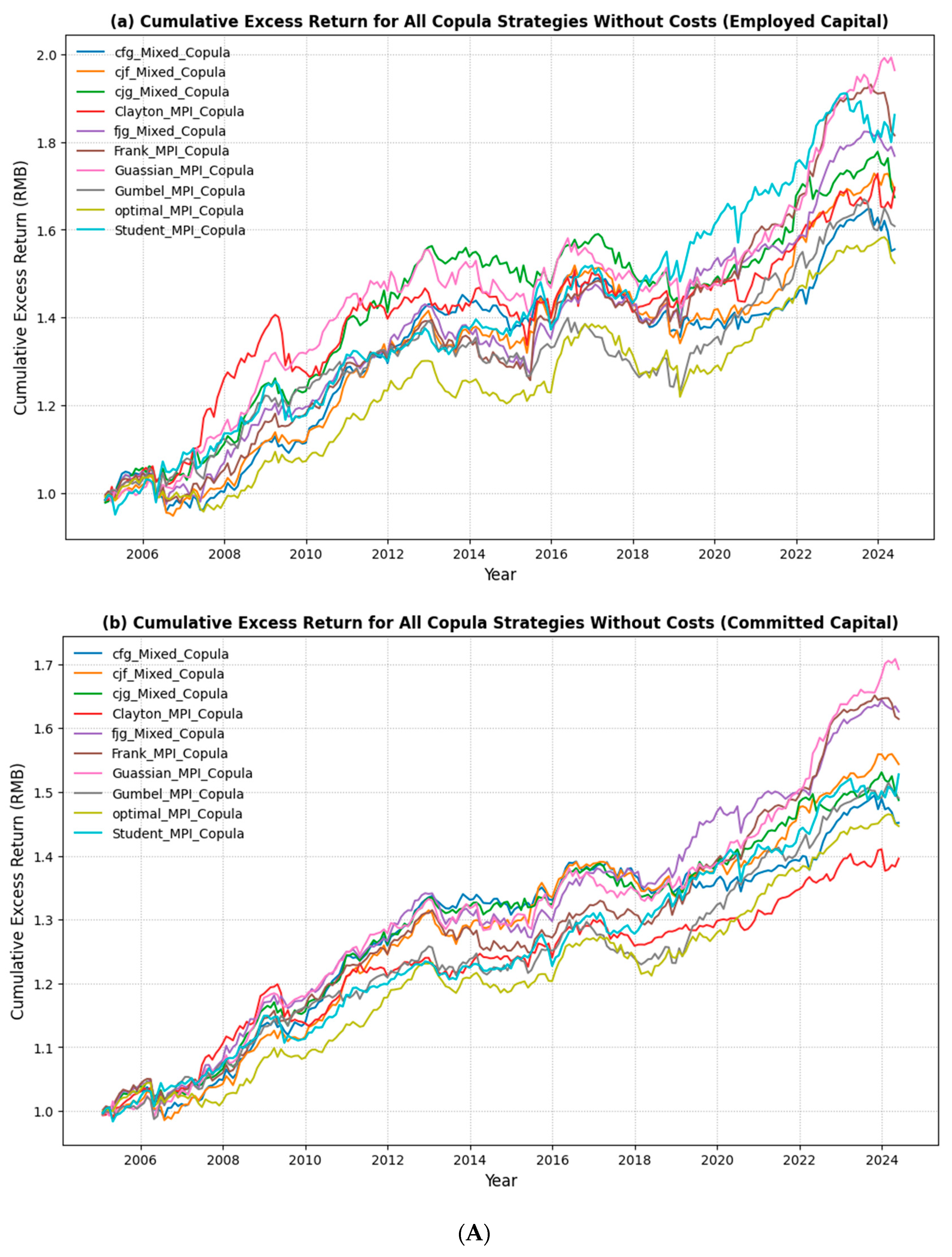
Before transaction costs (Table 2, Panel A), the SSD portfolios deliver the highest average monthly returns. The SSD-Hurst method achieves 0.84 percent and SSD-NZC method achieves 0.82 percent, with both significant at the 5 percent level. SSD-based strategies exhibit very high skewness and kurtosis, and the Jarque–Bera test strongly rejects normality for all methods. By contrast, among the copula-based strategies, the Gaussian copula unexpectedly generates the strongest results, with an average excess return of 0.30 percent and a Sharpe ratio of 0.23. This apparent superiority is somewhat surprising given that the Gaussian copula captures only linear dependence and lacks tail features. As shown later in Table 3, this advantage proves fragile once realistic frictions are incorporated. The Frank copula follows with 0.26 percent and a Sharpe ratio of 0.21, while Student’s t copula produces 0.28 percent and a Sharpe ratio of 0.19. The Clayton, Gumbel, and Optimal copulas perform more modestly, with mean returns in the range of 0.19 to 0.24 percent and Sharpe ratios slightly below those of Gaussian, Frank, and Student’s t.

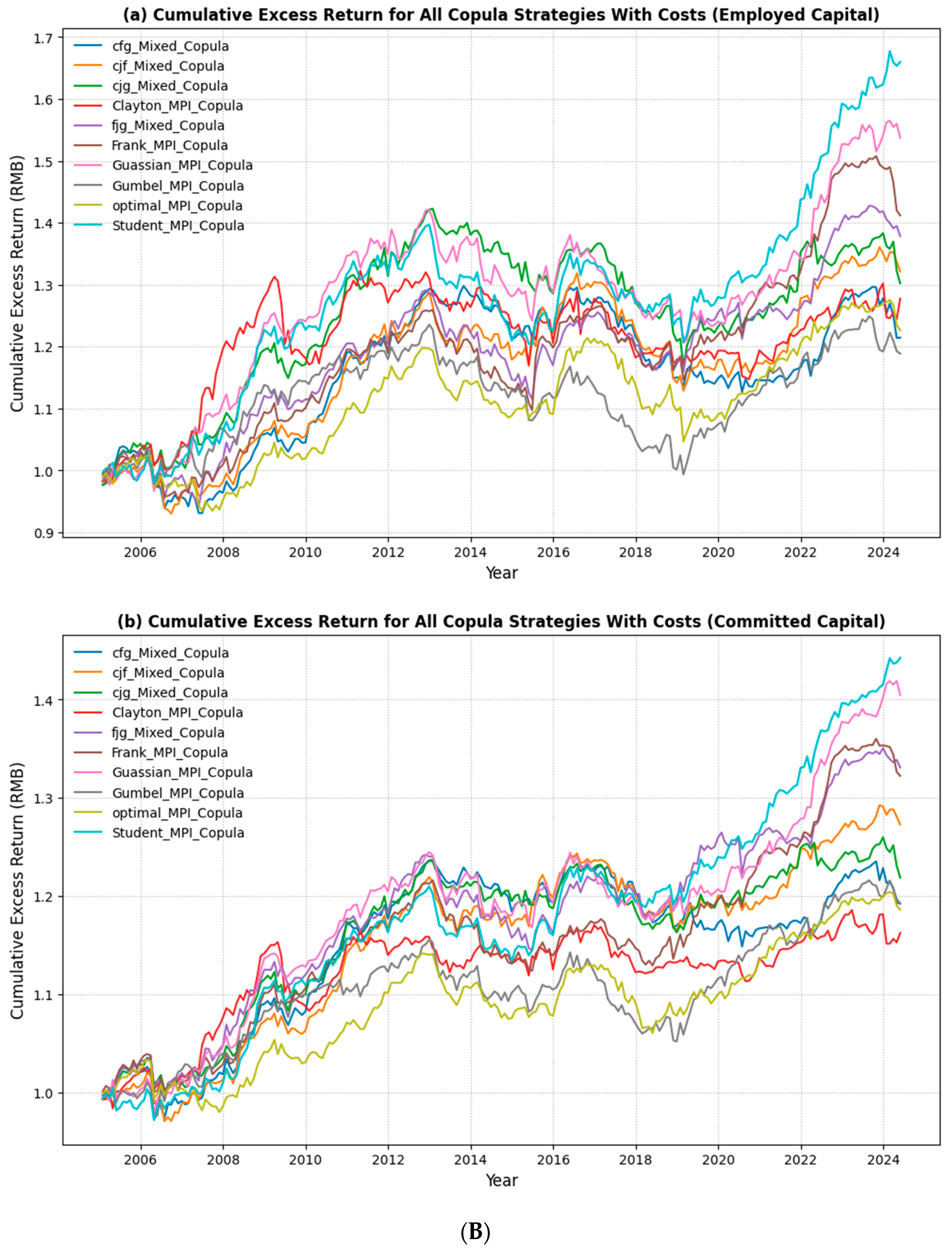
After transaction costs (Table 3, Panel A), average returns decline for all strategies. SSD-Hurst and SSD-NZC methods remain strong, posting 0.81 percent and 0.77 percent, respectively, both still significant at the 5 percent level. Several copula methods weaken: Clayton and Gumbel lose statistical significance, and Frank falls to marginal significance with a return of 0.16 percent and a t-statistic of 1.84. By contrast, Gaussian and Student’s t copulas remain significant, recording 0.19 percent and 0.23 percent with t-statistics of 2.37 and 2.69. These two methods demonstrate resilience to trading frictions relative to other copulas.

In terms of risk-adjusted performance after costs, Student’s t copula achieves a Sharpe ratio of 0.18, the Gaussian copula reaches 0.15, and SSD-Hurst method achieves 0.20, while the remaining copulas decline to levels near 0.07–0.08. The superior performance of Gaussian and Student’s t models reflects their ability to capture the most relevant dependence patterns in the data: linear co-movements in the case of the Gaussian copula and joint tail behavior in the case of Student’s t copula. In contrast, the Frank, Clayton, and Gumbel copulas provide only symmetric or one-sided tail dependence, which appears less aligned with market conditions and therefore less profitable. The Optimal copula, despite its adaptive design, performs worse than the Gaussian and Student’s t, a result that may reflect model-selection instability and limited out-of-sample generalization.

Transaction costs materially reduce strategy performance. For methods with modest pre-cost returns, such as Clayton and Gumbel, significance disappears once costs are included, underscoring their limited practical viability. By contrast, the SSD strategies continue to deliver high returns, but their extreme skewness and kurtosis point to severe tail risk, implying that occasional large losses remain hidden behind the mean–variance metrics.

Although the Gaussian copula appears to generate the highest average monthly excess return (0.30%) and Sharpe ratio (0.23) before accounting for transaction costs (Table 2), this superiority does not persist once realistic frictions are incorporated. After transaction costs are considered (Table 3), the Student-t copula consistently outperforms the Gaussian copula in both average returns and risk-adjusted measures, which highlights the lack of robustness of the Gaussian copula. Several factors can explain this discrepancy. First, the Gaussian copula captures only linear dependence and tends to produce more frequent trading signals, many of which may be noise-driven. While this increases pre-cost profitability, the higher turnover makes the strategy particularly vulnerable to transaction costs. Second, the Gaussian copula fails to account for tail dependence, which is prominent in equity returns as evidenced by the Jarque–Bera test rejecting normality at the 1% level. This limitation implies that the model underestimates the probability of extreme co-movements, leading to a higher likelihood of non-convergent trades and large losses once trading frictions are incorporated. Third, the apparent pre-cost outperformance of the Gaussian copula may be partly driven by spurious short-term correlations in the data that cannot be reliably exploited after costs. By contrast, the Student-t copula, which explicitly accommodates fat tails and joint extremes, produces fewer but higher-quality trading signals. This results in greater resilience to transaction costs and more stable post-cost performance. Overall, the evidence suggests that the Gaussian copula’s apparent advantage is not structural but sample-specific and fragile, whereas the Student-t copula provides a more reliable framework for capturing dependence structures in practice.

Beyond performance comparisons, this contradiction also has methodological implications. The apparent outperformance of the Gaussian copula suggests that even marginally mis-specified models can appear competitive when the data are dominated by linear co-movements. This further indicates that certain characteristics of our sample—such as periods of relative market stability outside crises—may favor models capturing only linear dependence. However, the fragility of this advantage once costs are incorporated highlights the importance of selecting copulas aligned with the true dependence structure, particularly under conditions of tail risk.

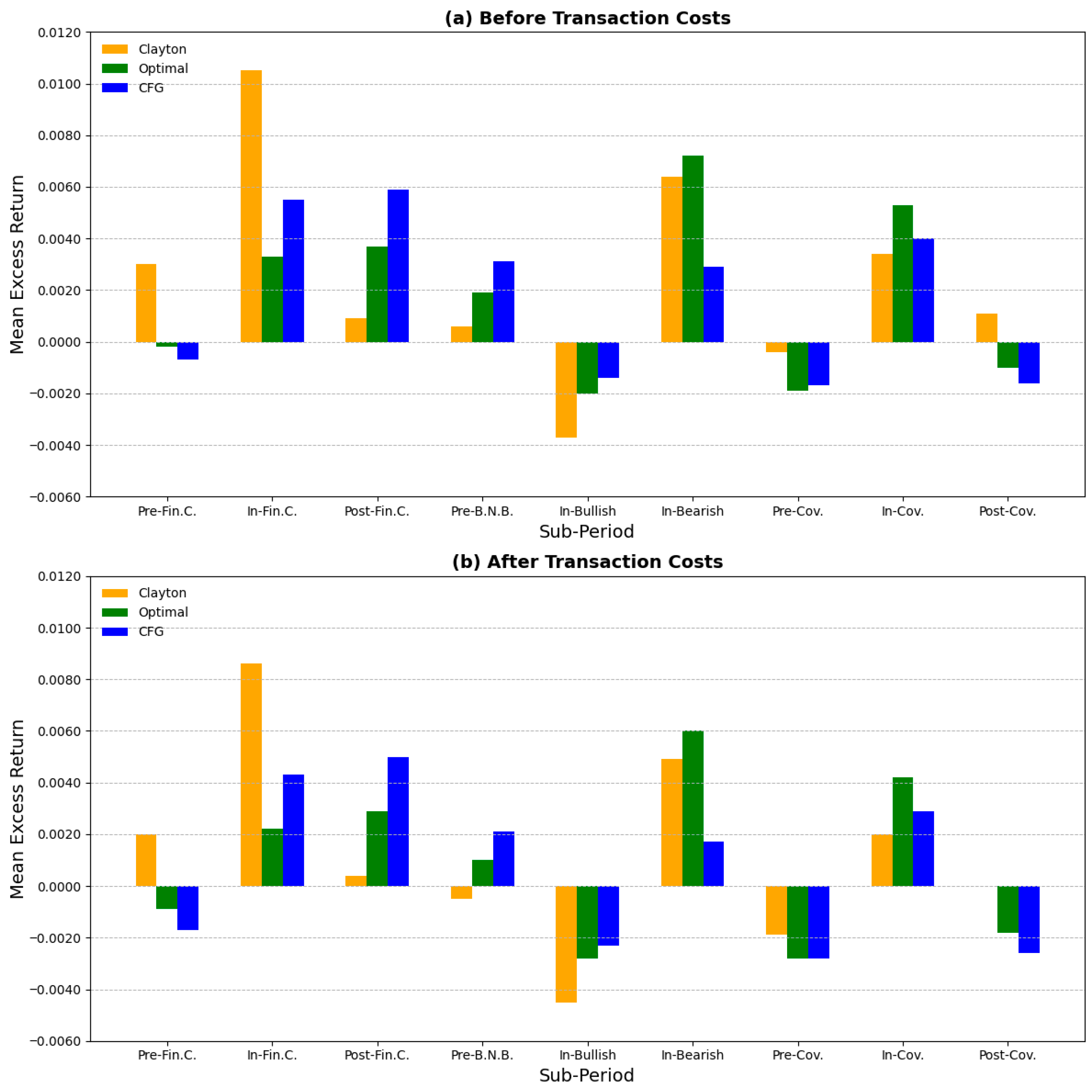
The table in Section 5.5 further reveals that the relative performances of copula-based strategies vary substantially across different market regimes. In tranquil periods, the Gaussian copula often delivers competitive results, reflecting its ability to capture dominant linear co-movements. However, during turbulent episodes characterized by heightened tail risk—such as the Global Financial Crisis (2007–2008), the Chinese stock market crash (2015–2016), and the COVID-19 pandemic (2020–2022)—the Student-t copula consistently outperforms the Gaussian copula. This superiority arises from the Student-t copula’s ability to model joint tail dependence, which becomes particularly relevant when extreme co-movements dominate equity returns. For instance, while the Gaussian copula records an average monthly return of 0.36% during the 2015–2016 bearish period, the Student-t copula achieves 0.55%. Similarly, in the COVID-19 crisis period, the Student-t copula yields 0.61%, compared with 0.58% for the Gaussian copula, and in the post-COVID recovery, the gap widens further (0.25% versus 0.04%). These results highlight that the apparent pre-cost advantage of the Gaussian copula is fragile and largely confined to stable regimes, whereas models with tail dependence, such as the Student-t copula, provide more reliable performance under stress conditions.

The performance differences among copula methods largely reflect the dependence structures that they capture. Gaussian and Student’s t copulas prove the most robust both before and after costs, since the former exploits dominant linear co-movements while the latter accounts for joint extremes. By contrast, Clayton and Gumbel emphasize one-sided tail dependence that appears less relevant in this market, and the Frank copula’s symmetry offers limited value. These findings underscore the importance of choosing a copula consistent with the true dependence patterns of asset pairs. Moreover, once realistic trading frictions are incorporated, strategies with modest pre-cost returns lose viability, and although SSD strategies retain high returns, their extreme skewness and kurtosis reveal substantial tail risk.

Finally, although our data clearly deviate from normality—as indicated by significant Jarque–Bera tests and non-zero skewness and excess kurtosis—the Gaussian copula remains competitive in some settings. This does not contradict statistical theory, because copulas separate the modeling of marginals from dependence. A Gaussian copula does not assume Gaussian marginals; rather, it assumes that dependence can be adequately summarized by linear correlation on the rank scale. In tranquil periods where tail dependence is weak and linear co-movements dominate, such an assumption can be effective, which explains the Gaussian copula’s pre-cost edge. Empirically, this edge arises because Gaussian-based strategies generate more trading signals, leading to higher gross returns but also greater turnover. Once realistic frictions are incorporated, however, the higher turnover translates into larger cost drag, and the Gaussian copula loses ground. Consistent with this mechanism, the Student-t copula consistently outperforms the Gaussian copula after costs in both average returns (0.23% vs. 0.19% per month) and Sharpe ratios (0.18 vs. 0.15), highlighting that the Gaussian advantage is fragile rather than structural.

The regime analysis reinforces this interpretation. In calm markets, the Gaussian copula remains competitive because linear co-movements dominate, but during stress episodes—such as the Global Financial Crisis (2007–2008), the Chinese crash (2015–2016), and the COVID-19 pandemic (2020–2022)—the Student-t copula systematically outperforms, owing to its ability to capture joint tail dependence. For instance, the Student-t copula achieves 0.55% versus 0.36% for Gaussian during the 2015–2016 downturn, and 0.61% versus 0.58% during the COVID-19 crisis. These findings suggest that Gaussian copulas can appear competitive under low-tail-dependence regimes, but models with explicit tail features provide more reliable performance when extreme co-movements dominate.

Methodologically, this implies that even mis-specified dependence structures may look appealing in certain subsamples, but their apparent advantages are not robust. Our results underscore that Gaussian copulas exploit dominant linear dependence but fail to accommodate extreme events, while the Student-t copula delivers a more reliable framework for practical applications where transaction costs and crisis regimes matter.

To provide further insights into the relative performances of copula-based strategies, Figure 3A,B present the cumulative excess returns from 2005 to 2024. Figure 3A reports results without transaction costs, while Figure 3B incorporates transaction costs, offering a more realistic assessment of profitability. In both figures, Panel (a) depicts returns based on employed capital and Panel (b) shows returns on committed capital.

Across both settings, the strategies exhibit gradual wealth accumulation starting from an initial investment of RMB 1, but their performances diverge over time. Without costs, several strategies—such as the Gaussian MPI Copula, Student-t MPI Copula, and Gumbel MPI Copula—achieve relatively higher cumulative returns by the end of the sample. Once transaction costs are included, overall profitability declines, with only a subset of copula-based methods maintaining notable excess returns. This comparison highlights the sensitivity of copula-based trading performance to transaction costs and underscores the importance of accounting for capital definitions when evaluating strategy outcomes.

Figure 4 presents the rolling 3-year Sharpe ratio for the same three strategies, providing insight into their risk-adjusted performance over time. The DM SSD-Hurst strategy again maintains superior performance, with its Sharpe ratio consistently higher than the other two strategies, particularly from 2009 to 2016. However, the performance gap narrows after 2020, with the student-t MPI Copula strategy showing notable improvement in its Sharpe ratio, even approaching the DM SSD-Hurst strategy around 2022. The FJG Mixed Copula strategy, while consistently lower in terms of Sharpe ratio, exhibits a gradual upward trend toward the end of the period. Overall, while the DM SSD-Hurst strategy leads in both cumulative return and risk-adjusted performance, the gap between the strategies, particularly in risk-adjusted terms, becomes less pronounced in the later years.

Figure 5 displays the distribution of trade returns after accounting for transaction costs for each strategy. All strategies show a noticeable leftward skew, indicating that extreme negative returns are more common than extreme positive returns. This is largely due to the fact that trades are generally closed when they converge based on predefined criteria. However, trades that do not converge remain open throughout the trading period, leading to the potential accumulation of losses. In rare cases, higher profits can occur when a pair’s price spread unexpectedly diverges by more than the threshold required to trigger the trade. A similar dynamic can occur when a pair converges, yielding larger-than-expected profits. Conversely, non-converging trades can result in significant losses before being forcibly closed by the strategy at the end of the trading period, contributing to the fat left tails seen in the distributions.

For strategies like the DM and cointegration methods, where trade entry and exit decisions are directly based on stock price movements, the scale of profit per trade is largely determined by the degree of divergence used to open the position. As a result, the potential for large gains is constrained, and the right tails of the distributions are relatively thin.

In contrast, the copula method, where trade entry and exit are based on the probability of relative mispricing between pairs rather than absolute price levels, shows a broader potential for positive returns, which can explain the slightly fatter right tail in its distribution. In practice, the application of a stop-loss mechanism could help mitigate extreme losses, giving copula-based strategies the potential to perform well without being capped by a fixed threshold for profitability. This flexibility allows for higher gains when the strategy is correct, although it also exposes the strategy to greater risks.

Statistical Significance Tests

This subsection evaluates whether monthly excess returns differ across the copula-based strategies, under both capital conventions and after accounting for transaction costs. The tests are conducted on the full monthly sample spanning 2005 to 2024, which provides 233 observations consistent with the dataset used in the rest of the study. Returns are defined according to the measures of employed capital and committed capital presented in Section 4.6. Because the return distributions exhibit strong departures from normality, as indicated by Jarque–Bera tests with p-values close to zero across all strategies, both parametric and non-parametric procedures are applied. Variance homogeneity is also examined to ensure robustness.

It is worth clarifying that the DMs are not included in the main set of significance tests. The reason is that these methods are fundamentally different from copula-based constructions and therefore do not serve as comparable alternatives within the same family of dependence models. To verify this, additional pairwise t-tests are performed between the DM-based strategies and each copula strategy. The results consistently indicate statistically significant mean differences, confirming that the DM procedures belong to a distinct methodological class rather than representing minor variants of the copula framework. For transparency, the detailed outcomes of these pairwise comparisons are reported in Appendix A 

Table A4. Statistical Significance of Performance Differences Across Copulas.

Test	t-Statistic	p-Value	Conclusion
Panel I-A: Return on employed capital without costs
ANOVA	0.1736	0.9966	$\mathrm{Fail}\mathrm{to}\mathrm{reject}{H}_0$, no mean differences.
Kruskal–Wallis	1.9354	0.9924	No significant distributional differences.
Friedman	4.7450	0.8559	No rank differences.
Levene	1.2525	0.2581	No evidence of heteroskedasticity.
Welch ANOVA	0.1826	0.9959	$\mathrm{Fail}\mathrm{to}\mathrm{reject}{H}_0$, no mean differences.
Panel I-B: Return on committed capital without costs
ANOVA	0.3302	0.9653	$\mathrm{Fail}\mathrm{to}\mathrm{reject}{H}_0$, no mean differences.
Kruskal–Wallis	4.0392	0.9088	No significant distributional differences.
Friedman	6.2713	0.7125	No rank differences.
Levene	0.6023	0.7961	No evidence of heteroskedasticity.
Welch ANOVA	0.3245	0.9671	$\mathrm{Fail}\mathrm{to}\mathrm{reject}{H}_0$, no mean differences.
Panel II-A: Return on employed capital with costs
ANOVA	0.3274	0.9662	$\mathrm{Fail}\mathrm{to}\mathrm{reject}{H}_0$, no mean differences.
Kruskal–Wallis	2.0585	0.9905	No significant distributional differences.
Friedman	4.9191	0.8413	No rank differences.
Levene	0.8954	0.5285	No evidence of heteroskedasticity.
Welch ANOVA	0.3289	0.9656	$\mathrm{Fail}\mathrm{to}\mathrm{reject}{H}_0$, no mean differences.
Panel II-B: Return on committed capital with costs
ANOVA	0.5299	0.8538	$\mathrm{Fail}\mathrm{to}\mathrm{reject}{H}_0$, no mean differences.
Kruskal–Wallis	5.1239	0.8234	No significant distributional differences.
Friedman	12.7813	0.1728	No rank differences.
Levene	0.5623	0.8288	No evidence of heteroskedasticity.
Welch ANOVA	0.5193	0.8612	$\mathrm{Fail}\mathrm{to}\mathrm{reject}{H}_0$, no mean differences.

Note: Tests are performed on monthly excess returns from January 2005 to June 2024 (233 months) for the copula-based strategies only. Panels report results under (i) employed vs. committed capital and (ii) before vs. after transaction costs. Reported procedures: one-way ANOVA (H₀: equal means), Welch’s ANOVA (H₀: equal means under unequal variances), Levene’s test (H₀: equal variances), Kruskal–Wallis (H₀: identical distributions), and Friedman (H₀: identical median ranks across repeated measures). Given the strong non-normality of strategy returns (JB test p ≈ 0 across strategies), non-parametric tests complement the parametric analysis.

and

Table A5. Tukey HSD Multiple Comparisons of Mean Monthly Returns across Copula Strategies (Employed Capital, with Costs).

Group1	Group2	MeanDiff	p-Adj	Lower	Upper	Reject
CFG_Mixed_Copula	CJF_Mixed_Copula	0.0004	1.0000	−0.0032	0.0040	FALSE
CFG_Mixed_Copula	CJG_Mixed_Copula	0.0003	1.0000	−0.0033	0.0039	FALSE
CFG_Mixed_Copula	Clayton_Copula	0.0003	1.0000	−0.0034	0.0039	FALSE
CFG_Mixed_Copula	FJG_Mixed_Copula	0.0006	1.0000	−0.0031	0.0042	FALSE
CFG_Mixed_Copula	Frank_Copula	0.0007	0.9999	−0.0030	0.0043	FALSE
CFG_Mixed_Copula	Guassian_Copula	0.0010	0.9964	−0.0026	0.0047	FALSE
CFG_Mixed_Copula	Gumbel_Copula	−0.0001	1.0000	−0.0037	0.0035	FALSE
CFG_Mixed_Copula	Optimal_Copula	0.0000	1.0000	−0.0036	0.0037	FALSE
CFG_Mixed_Copula	Student_t_Copula	0.0014	0.9742	−0.0023	0.0050	FALSE
CJF_Mixed_Copula	CJG_Mixed_Copula	−0.0001	1.0000	−0.0037	0.0036	FALSE
CJF_Mixed_Copula	Clayton_Copula	−0.0001	1.0000	−0.0037	0.0035	FALSE
CJF_Mixed_Copula	FJG_Mixed_Copula	0.0002	1.0000	−0.0034	0.0038	FALSE
CJF_Mixed_Copula	Frank_Copula	0.0003	1.0000	−0.0033	0.0039	FALSE
CJF_Mixed_Copula	Guassian_Copula	0.0007	0.9999	−0.0030	0.0043	FALSE
CJF_Mixed_Copula	Gumbel_Copula	−0.0004	1.0000	−0.0041	0.0032	FALSE
CJF_Mixed_Copula	Optimal_Copula	−0.0003	1.0000	−0.0040	0.0033	FALSE
CJF_Mixed_Copula	Student_t_Copula	0.0010	0.9975	−0.0026	0.0046	FALSE
CJG_Mixed_Copula	Clayton_Copula	−0.0001	1.0000	−0.0037	0.0036	FALSE
CJG_Mixed_Copula	FJG_Mixed_Copula	0.0002	1.0000	−0.0034	0.0039	FALSE
CJG_Mixed_Copula	Frank_Copula	0.0003	1.0000	−0.0033	0.0040	FALSE
CJG_Mixed_Copula	Guassian_Copula	0.0007	0.9998	−0.0029	0.0043	FALSE
CJG_Mixed_Copula	Gumbel_Copula	−0.0004	1.0000	−0.0040	0.0032	FALSE
CJG_Mixed_Copula	Optimal_Copula	−0.0003	1.0000	−0.0039	0.0033	FALSE
CJG_Mixed_Copula	Student_t_Copula	0.0010	0.9961	−0.0026	0.0047	FALSE
Clayton_Copula	FJG_Mixed_Copula	0.0003	1.0000	−0.0033	0.0039	FALSE
Clayton_Copula	Frank_Copula	0.0004	1.0000	−0.0032	0.0040	FALSE
Clayton_Copula	Guassian_Copula	0.0008	0.9996	−0.0028	0.0044	FALSE
Clayton_Copula	Gumbel_Copula	−0.0003	1.0000	−0.0039	0.0033	FALSE
Clayton_Copula	Optimal_Copula	−0.0002	1.0000	−0.0038	0.0034	FALSE
Clayton_Copula	Student_t_Copula	0.0011	0.9939	−0.0025	0.0047	FALSE
FJG_Mixed_Copula	Frank_Copula	0.0001	1.0000	−0.0035	0.0037	FALSE
FJG_Mixed_Copula	Guassian_Copula	0.0005	1.0000	−0.0031	0.0041	FALSE
FJG_Mixed_Copula	Gumbel_Copula	−0.0006	0.9999	−0.0042	0.0030	FALSE
FJG_Mixed_Copula	Optimal_Copula	−0.0005	1.0000	−0.0041	0.0031	FALSE
FJG_Mixed_Copula	Student_t_Copula	0.0008	0.9995	−0.0028	0.0044	FALSE
Frank_Copula	Guassian_Copula	0.0004	1.0000	−0.0033	0.0040	FALSE
Frank_Copula	Gumbel_Copula	−0.0007	0.9998	−0.0044	0.0029	FALSE
Frank_Copula	Optimal_Copula	−0.0006	0.9999	−0.0042	0.0030	FALSE
Frank_Copula	Student_t_Copula	0.0007	0.9998	−0.0029	0.0043	FALSE
Guassian_Copula	Gumbel_Copula	−0.0011	0.9940	−0.0047	0.0025	FALSE
Guassian_Copula	Optimal_Copula	−0.0010	0.9974	−0.0046	0.0026	FALSE
Guassian_Copula	Student_t_Copula	0.0003	1.0000	−0.0033	0.0039	FALSE
Gumbel_Copula	Optimal_Copula	0.0001	1.0000	−0.0035	0.0037	FALSE
Gumbel_Copula	Student_t_Copula	0.0014	0.9634	−0.0022	0.0051	FALSE
Optimal_Copula	Student_t_Copula	0.0013	0.9793	−0.0023	0.0049	FALSE

Note: This table reports Tukey’s Honestly Significant Difference (HSD) test for pairwise mean comparisons of monthly returns among copula-based strategies, using the employed capital convention with transaction costs included. Each row contrasts two strategies (Group1 vs. Group2). The column MeanDiff shows the difference in average monthly returns between the two strategies, p-Adj is the adjusted p-value accounting for multiple testing, and Reject indicates whether the null hypothesis of equal means is rejected at the 5% family-wise error rate. For example, the first row compares CFG Mixed Copula and CJF Mixed Copula: the mean difference is 0.0004, the adjusted p-value is 1.0000, and the null is not rejected, indicating no significant difference.

.

The results for the employed capital measure without transaction costs show that neither ANOVA nor Welch ANOVA detects any difference in mean returns across the copula families. Likewise, the Kruskal–Wallis test does not identify any distributional differences, and the Friedman test suggests no differences in the relative ranking of strategies across time. Levene’s test indicates no evidence of heteroskedasticity. Taken together, these findings demonstrate that the copula-based strategies are statistically indistinguishable when evaluated under this capital convention.

When the analysis is repeated using the committed capital measure without costs, the same pattern emerges. Both ANOVA and Welch ANOVA point to an absence of mean return differences, while Kruskal–Wallis and Friedman tests corroborate the lack of distributional and rank-based gaps. Levene’s test again confirms that the variance structure is homogeneous. This reinforces the conclusion that the choice of capital convention does not alter the lack of significant performance differentials among copula families.

After incorporating trading costs, the results remain unchanged. For the employed capital specification with costs, all four hypothesis tests—ANOVA, Welch ANOVA, Kruskal–Wallis, and Friedman—fail to reject the null hypotheses, while Levene’s test indicates stable variance properties. Under the committed capital specification with costs, the outcomes are consistent: parametric tests detect no mean differences, non-parametric tests find no distributional or rank disparities, and Levene’s test again supports variance homogeneity.

Across all four panels, every test produces p-values far above conventional significance thresholds. The range of ANOVA results, for example, runs from 0.85 to nearly 1.00, while Welch ANOVA and non-parametric tests lead to similarly high values. Levene’s statistics also provide no indication of heteroskedasticity. This uniformity across methodologies suggests that the performance differences among copula families are not statistically meaningful, regardless of whether the evaluation is based on employed or committed capital, and irrespective of whether transaction costs are considered.

The broader implication is that although certain copulas such as Student-t or Gaussian may appear more resilient after costs when viewed through point estimates or Sharpe ratios, these apparent differences do not hold up under formal statistical testing. The convergence of parametric and non-parametric evidence strengthens the conclusion that no single copula family systematically dominates the others.

5.2. Risk Adjusted Performance

Given the non-normal distribution of returns in pairs trading strategies, relying solely on the Sharpe ratio may underestimate downside risk and overstate performance (Eling, 2008). To provide a more comprehensive evaluation, the analysis is supplemented with downside risk measures and drawdown-based performance metrics, as summarized in

Table 4. Overview of Risk-Adjusted Performance.

	Lower Partial Moments Measures			Drawdown Measures
	Omega	Sortino Ratio	Kappa 3	Max D.	Calmar Ratio	Sterling Ratio	Burke Ratio
Panel A: Before transaction costs
SSD-Hurst	5.0290	0.7395	0.6951	−0.0831	1.2767	7.1608	0.4977
SSD-NZC	3.4930	0.4769	0.4428	−0.0963	1.0745	4.1353	0.2782
Clayton	1.5983	0.1558	0.1637	−0.1005	0.2870	0.9600	0.0577
Frank	1.7884	0.2171	0.2312	−0.0988	0.3258	1.1411	0.0704
Gaussian	1.8122	0.2307	0.2610	−0.1014	0.3590	1.0808	0.0685
Gumbel	1.5314	0.1558	0.1688	−0.1208	0.2135	0.7163	0.0440
Student-t	1.6723	0.1762	0.1900	−0.0730	0.4637	1.4738	0.0917
Optimal	1.5375	0.1444	0.1509	−0.1197	0.1901	0.5929	0.0374
CFG	1.5689	0.1635	0.1816	−0.0953	0.2497	0.6288	0.0393
CJF	1.6587	0.1738	0.1891	−0.1171	0.2424	0.7158	0.0460
CJG	1.6131	0.1699	0.1906	−0.1258	0.2217	0.9192	0.0546
FJG	1.7169	0.2053	0.2150	−0.1112	0.2765	1.0946	0.0656
Panel B: After transaction costs
SSD-Hurst	4.7299	0.7982	0.7966	−0.0675	1.4971	6.2675	0.4372
SSD-NZC	3.2149	0.4462	0.4099	−0.0973	0.9916	3.6369	0.2368
Clayton	1.2642	0.0795	0.0794	−0.1326	0.1045	0.2431	0.0145
Frank	1.4204	0.1282	0.1334	−0.1284	0.1470	0.5225	0.0306
Gaussian	1.4832	0.1495	0.1670	−0.1516	0.1542	0.4257	0.0247
Gumbel	1.1852	0.0603	0.0639	−0.1960	0.0506	0.1553	0.0086
Student-t	1.5929	0.1805	0.2079	−0.1382	0.1982	0.5405	0.0319
Optimal	1.2470	0.0759	0.0766	−0.1379	0.0822	0.2501	0.0141
CFG	1.2379	0.0739	0.0806	−0.1320	0.0818	0.1961	0.0113
CJF	1.3254	0.0956	0.1016	−0.1439	0.1068	0.2917	0.0173
CJG	1.2967	0.0901	0.0999	−0.1788	0.0818	0.2418	0.0143
FJG	1.3761	0.1174	0.1210	−0.1362	0.1288	0.4162	0.0245

Note: This table provides an overview of key risk-adjusted performance measures for the monthly employed capital excess returns of various pairs trading strategies, including SSD-Hurst, SSD-NZC, and several copula-based strategies. Panel A shows the results before transaction costs, while Panel B presents the results after transaction costs. The performance metrics include lower partial moments (Omega ratio, Sortino ratio, Kappa 3) and drawdown measures (Max Drawdown, Calmar ratio, Sterling ratio, Burke ratio).

.

Before transaction costs, the SSD-Hurst strategy demonstrates the strongest performance across all downside risk metrics. It records the highest Omega ratio (5.03), indicating that returns above the threshold substantially outweigh those below. Its Sortino ratio (0.74) and Kappa 3 ratio (0.70) further highlight superior risk-adjusted performance when accounting for downside volatility and skewness. The SSD-NZC strategy also performs well, though noticeably weaker than SSD-Hurst, reaffirming the latter’s dominance in managing downside risk.

Among the copula-based strategies, the Gaussian and FJG copulas deliver the most favorable downside risk profiles. Both achieve relatively high Sortino and Kappa 3 ratios, reflecting solid performance when downside deviations are emphasized. In contrast, the Clayton and Gumbel copulas underperform across all downside risk metrics, with low Omega ratios and suppressed Sortino and Kappa 3 values. This suggests that these strategies are less effective at generating returns that sufficiently compensate for downside exposure.

Turning to drawdown metrics, the SSD-Hurst method continues to outperform, showing a moderate maximum drawdown of −8.3% and the highest Calmar (1.28), Sterling (7.16), and Burke (0.50) ratios. These results suggest that the strategy achieves a strong return profile relative to drawdown risks. Among copula methods, the Student-t copula records the smallest maximum drawdown (−7.3%) and maintains a relatively strong Calmar ratio, indicating effective tail-risk management, likely due to its ability to model extreme co-movements.

After incorporating transaction costs, all strategies experience a decline in performance, but the degree of impact varies. The SSD-Hurst method remains the most resilient: while its Omega ratio declines slightly (to 4.73), its Sortino ratio improves marginally, and its drawdown-related metrics remain robust. This suggests that SSD-Hurst method not only delivers high risk-adjusted returns but is also less sensitive to trading frictions. The strategy’s relatively low turnover may help limit the erosion of returns caused by costs.

In contrast, copula-based strategies—particularly Clayton and Gumbel—show sharp deterioration. Their Omega ratios fall below 1.3, and Sortino ratios decline by nearly half, rendering the strategies ineffective after transaction costs. The Gaussian and Student-t copulas, however, retain partial robustness. Although their risk-adjusted metrics decline, they remain more stable than other copula-based methods, affirming the benefit of capturing broader dependence structures.

The variation in risk-adjusted performance can largely be attributed to the dependence structure modeled by each copula. The Gaussian copula, which captures linear correlation, performs consistently well, suggesting that such relationships are dominant in the data. The Student-t copula, which captures both linear and tail dependencies, provides a more comprehensive modeling of co-movements, especially during market extremes. In contrast, Clayton and Gumbel copulas, which focus on lower and upper tail dependence, respectively, may not align well with the actual structure of profitable trading opportunities in this dataset. The Frank copula, with symmetric but no tail dependence, delivers moderate results.

In summary, the SSD-Hurst strategy emerges as the most robust across all risk-adjusted metrics, outperforming both the SSD-NZC and copula-based strategies, regardless of whether transaction costs are considered. Among copula approaches, the Student-t copula stands out for its relative stability and effective risk control. These findings underscore the importance of aligning the dependence structure in modeling with the characteristics of the actual data and highlight that transaction costs remain a critical constraint, particularly for high-turnover strategies. A comprehensive evaluation of pairs trading strategies must therefore integrate both advanced dependence modeling and realistic cost considerations.

5.3. Risk Characteristics of Pairs Trading Strategies

To further understand the economic drivers behind the findings and to assess whether the profitability of pairs trading is a compensation for risk, a regression of daily excess returns on various risk factors is performed. Specifically, this study uses Fama and French’s (2015) five-factor model, which includes the excess return on a broad market portfolio (Rm − Rf), the difference between the return on small-cap stocks and large-cap stocks (SMB), the difference between the return on high book-to-market stocks and low book-to-market stocks (HML), the difference in returns between the most profitable and least profitable stocks (RMW), and the difference in returns between conservatively investing firms and aggressively investing firms (CMA). In addition, the momentum (MOM) and long-term reversal (REV) factors are also included.

The model is structured as follows:

$$R_{i,t}-R_{f,t}={\alpha }_i+{\beta }_i(R_{m,t}-R_{f,t})+s_i{SMB}_t+h_i{HML}_t+r_i{RMW}_t+c_i{CMA}_t+m_i{Mom}_t+l_i{Rev}_t+{ϵ}_{i,t}$$

(17)

where $i$ denotes the portfolio, and $t$ represents time. The error terms ${ϵ}_{i,t}$ are assumed to have a mean of zero and are uncorrelated over time. Heteroscedasticity and autocorrelation adjustments are made using the Newey-West method, with a lag length of six.

Table 5. Monthly risk profile based on Fama and French five factors plus Momentum and Long-Term Reversal.

Strategy	Alpha	MKT	SMB	HML	RMW	CMA	MOM	REV
Panel A: Before transaction costs
SSD-Hurst	0.0052	0.0049	0.1828	0.1314	0.0465	−0.2632	−0.0729	−0.0486
SSD-NZC	0.0055	0.0028	0.1851	0.1573	0.0729	−0.2967 *	−0.0663	−0.0251
Clayton	−0.0006	−0.0041	0.2059 **	0.1080	0.1016	−0.1966 *	0.0042	0.0126
Frank	0.0011	−0.0202	0.1178	0.0438	0.1051	−0.0702	−0.0127	0.0244
Gaussian	0.0011	−0.0078	0.1126	0.0917	0.0538	−0.1167	0.0284	0.0231
Gumbel	0.0001	−0.0097	0.1345	0.0674	0.1057	−0.1160	0.0024	0.0147
Student-t	0.0009	0.0075	0.0691	0.0280	0.0359	−0.1030	−0.0243	0.0093
Optimal	−0.0003	−0.0156	0.1721 *	0.0945	0.0981	−0.1220	0.0065	0.0233
CFG	0.0001	−0.0088	0.1418	0.0080	0.0812	−0.0861	−0.0010	0.0278
CJF	0.0001	−0.0036	0.1585	0.0662	0.1182	−0.1029	−0.0119	0.0188
CJG	0.0000	−0.0092	0.1815 *	0.0761	0.0963	−0.0951	0.0037	0.0205
FJG	0.0005	−0.0199	0.1506	0.0436	0.1096	−0.1086	−0.0045	0.0257
Panel B: After transaction costs
SSD-Hurst	0.0048	0.0046	0.1811	0.1314	0.0457	−0.2652	−0.0705	−0.0476
SSD-NZC	0.0049	0.0025	0.1865	0.1577	0.0725	−0.2973 *	−0.0653	−0.0238
Clayton	−0.0018	−0.0028	0.1993 **	0.0998	0.0988	−0.1881 *	0.0053	0.0133
Frank	0.0000	−0.0182	0.1181	0.0421	0.1044	−0.0717	−0.0125	0.0245
Gaussian	0.0000	−0.0075	0.1123	0.0915	0.0507	−0.1207	0.0257	0.0236
Gumbel	−0.0013	−0.0097	0.1366	0.0704	0.1010	−0.1240	0.0028	0.0142
Student-t	0.0004	−0.0129	0.1234	0.0458	0.0954	−0.0782	0.0055	0.0263
Optimal	−0.0013	−0.0119	0.1682 *	0.0891	0.0964	−0.1173	0.0042	0.0241
CFG	−0.0010	−0.0077	0.1446	0.0094	0.0831	−0.0883	−0.0003	0.0275
CJF	−0.0010	−0.0026	0.1602 *	0.0651	0.1178	−0.1043	−0.0133	0.0178
CJG	−0.0011	−0.0064	0.1825 *	0.0783	0.0943	−0.1011	0.0041	0.0204
FJG	−0.0006	−0.0186	0.1516	0.0414	0.1123	−0.1076	−0.0045	0.0256

Note: This table presents the results of regressing the monthly returns of various pairs trading strategies on the Fama–French five-factor model augmented with Momentum and Long-Term Reversal factors. Panel A reports the regression coefficients before accounting for transaction costs, while Panel B reports the coefficients after transaction costs. The column labeled ‘Alpha’ represents the estimated regression intercept, indicating the strategy’s average abnormal return not explained by the included factors. The columns ‘MKT’, ‘SMB’, ‘HML’, ‘RMW’, ‘CMA’, ‘MOM’, and ‘REV’ report the estimated coefficients for the following factors, respectively: MKT: Market Excess Return (Market Risk Premium), SMB: Small Minus Big (size factor), HML: High Minus Low (value factor), RMW: Robust Minus Weak (profitability factor), CMA: Conservative Minus Aggressive (investment factor), MOM: Momentum factor, REV: Long-Term Reversal factor. * significant at the 10% level. ** significant at the 5% level.

reports regression results assessing whether the profits from pairs trading strategies are attributable to common risk factors or represent abnormal returns. In Panel A (before transaction costs), the SSD-Hurst and SSD-NZC strategies exhibit positive alphas of 0.0052 and 0.0055, respectively, indicating average monthly excess returns of 0.52% and 0.55% unexplained by the included factors—evidence of strong risk-adjusted performance. In contrast, most copula-based strategies show smaller and less significant alphas. For example, the Clayton strategy has a negative alpha of −0.0006, suggesting that its returns are either fully captured by risk exposures or lack meaningful abnormal profits.

The coefficients on the MKT factor are close to zero or negative for most strategies, indicating minimal exposure to market risk. This aligns with the market-neutral nature of pairs trading strategies, which typically involve taking offsetting long and short positions to eliminate the influence of market movements. The SMB factor coefficients are positive for all strategies and statistically significant for some. For example, the Clayton strategy has a significant SMB coefficient of 0.2059 ** before costs and 0.1993 ** after costs, suggesting a bias toward small-cap stocks. This may be because smaller companies present more mispricing opportunities due to lower analyst coverage and liquidity. The HML factor coefficients are positive across all strategies but not statistically significant, indicating a mild exposure to value stocks but not a strong determinant of returns.

Regarding the RMW factor, the coefficients are positive but generally insignificant, indicating that the strategies do not have substantial exposure to firms with varying profitability levels. The CMA factor shows negative coefficients for all strategies, with the SSD-NZC strategy exhibiting a significant negative coefficient (−0.2967 * before costs and −0.2973 * after costs). A negative CMA coefficient implies that the strategies are tilted toward firms with aggressive investment policies, potentially capitalizing on inefficiencies associated with such firms. The MOM factor coefficients are mostly negative but insignificant, indicating that the strategies may benefit slightly from contrarian positions against momentum stocks, which is consistent with the mean-reversion nature of pairs trading. The REV factor coefficients are small and not statistically significant, suggesting that long-term reversal effects do not play a significant role in the strategies’ returns.

In Panel B (after transaction costs), the alphas for the SSD-Hurst and SSD-NZC strategies remain positive at 0.0048 and 0.0049, respectively, though slightly reduced due to trading costs. This persistence indicates that these strategies continue to generate abnormal returns even after accounting for transaction costs. The copula-based strategies’ alphas become more negative or remain small after costs, highlighting the sensitivity of these strategies to transaction costs and potentially lower profitability.

Transaction costs have a noticeable impact on the profitability of the strategies, particularly for those with lower alphas or higher turnover rates. The SSD-Hurst and SSD-NZC strategies maintain positive alphas after costs, suggesting that their trading frequency and associated costs do not significantly erode their abnormal returns. In contrast, some copula-based strategies experience a reduction in alpha, indicating that transaction costs may outweigh the gains from these strategies.

The positive and significant SMB coefficients for some strategies indicate an exposure to small-cap stocks, which may contribute to their returns. This exposure could arise from the selection of stock pairs involving smaller firms or from exploiting inefficiencies prevalent in the small-cap segment. The negative CMA coefficients suggest a tendency to invest in firms with aggressive investment practices. These firms might offer more opportunities for mispricing due to their growth-oriented strategies and potentially higher volatility. The minimal exposure to the MKT factor across strategies confirms their market-neutral stance, making them attractive for diversification purposes in a portfolio context.

The regression analysis reveals that the profitability of the SSD-Hurst and SSD-NZC strategies cannot be fully explained by common risk factors, as evidenced by their significant positive alphas before and after transaction costs. These strategies appear to capture unique sources of return, possibly linked to market inefficiencies or behavioral biases not accounted for by traditional risk factors. For the copula-based strategies, the results are mixed. While some show positive alphas before costs, these gains are often offset by transaction costs, reducing their effectiveness. The significant exposure to the SMB factor in certain copula strategies indicates that returns may be partially driven by size-related risks rather than pure arbitrage opportunities. Overall, the findings suggest that pairs trading strategies, particularly those based on stochastic dominance (SSD-Hurst and SSD-NZC methods), offer risk-adjusted returns that are not solely compensation for bearing systematic risk.

5.4. Robustness and Sensitivity Analysis

5.4.1. Varying Opening Thresholds

In the previous analyses, a constant opening threshold of 0.6 was applied for the copula-based trading strategies. To evaluate the robustness of these strategies and understand how different opening thresholds affect their performance, a sensitivity analysis was conducted by varying the opening thresholds from 0.2 to 0.8 in increments of 0.1.

Table 6. Copula Method’s Sensitivity Analysis with Various Opening Threshold for Committed Capital Return After Trading Costs.

Strategy		0.2	0.3	0.4	0.5	0.6	0.7	0.8
Clayton	Mean	0.0001	0.0003	0.0003	0.0005	0.0007	0.0008	0.0007
	Min	−0.0415	−0.0401	−0.0360	−0.0339	−0.0323	−0.0351	−0.0323
	Max	0.0240	0.0304	0.0261	0.0199	0.0239	0.0231	0.0242
	Std. Dev.	0.0088	0.0087	0.0080	0.0072	0.0069	0.0067	0.0062
Frank	Mean	0.0014	0.0015	0.0015	0.0013	0.0012	0.0013	0.0011
	Min	−0.0491	−0.0427	−0.0442	−0.0378	−0.0355	−0.0331	−0.0348
	Max	0.0214	0.0258	0.0203	0.0178	0.0154	0.0167	0.0165
	Std. Dev.	0.0085	0.0084	0.0080	0.0071	0.0069	0.0067	0.0063
Gaussian	Mean	0.0016	0.0016	0.0016	0.0015	0.0015	0.0015	0.0015
	Min	−0.0384	−0.0344	−0.0336	−0.0323	−0.0276	−0.0270	−0.0248
	Max	0.0363	0.0334	0.0320	0.0307	0.0244	0.0235	0.0223
	Std. Dev.	0.0093	0.0087	0.0082	0.0078	0.0072	0.0069	0.0065
Gumbel	Mean	0.0004	0.0007	0.0007	0.0007	0.0008	0.0007	0.0006
	Min	−0.0433	−0.0432	−0.0404	−0.0342	−0.0305	−0.0302	−0.0266
	Max	0.0249	0.0364	0.0326	0.0295	0.0269	0.0211	0.0150
	Std. Dev.	0.0090	0.0089	0.0085	0.0074	0.0072	0.0068	0.0063
Student-t	Mean	0.0020	0.0020	0.0017	0.0017	0.0016	0.0015	0.0016
	Min	−0.0304	−0.0296	−0.0279	−0.0283	−0.0248	−0.0252	−0.0257
	Max	0.0301	0.0325	0.0268	0.0249	0.0294	0.0302	0.0261
	Std. Dev.	0.0087	0.0084	0.0080	0.0073	0.0070	0.0067	0.0063
Optimal	Mean	0.0012	0.0010	0.0009	0.0008	0.0008	0.0007	0.0005
	Min	−0.0490	−0.0431	−0.0458	−0.0379	−0.0368	−0.0336	−0.0367
	Max	0.0212	0.0195	0.0182	0.0177	0.0133	0.0163	0.0133
	Std. Dev.	0.0080	0.0077	0.0074	0.0066	0.0063	0.0059	0.0056
CFG	Mean	0.0009	0.0010	0.0008	0.0009	0.0008	0.0009	0.0007
	Min	−0.0422	−0.0371	−0.0376	−0.0320	−0.0297	−0.0258	−0.0273
	Max	0.0267	0.0233	0.0212	0.0222	0.0201	0.0166	0.0152
	Std. Dev.	0.0087	0.0083	0.0078	0.0070	0.0067	0.0062	0.0058
CJF	Mean	0.0012	0.0011	0.0010	0.0011	0.0011	0.0011	0.0010
	Min	−0.0407	−0.0352	−0.0291	−0.0278	−0.0260	−0.0262	−0.0269
	Max	0.0281	0.0234	0.0221	0.0220	0.0216	0.0203	0.0174
	Std. Dev.	0.0086	0.0082	0.0076	0.0072	0.0068	0.0063	0.0058
CJG	Mean	0.0014	0.0013	0.0012	0.0010	0.0009	0.0008	0.0008
	Min	−0.0364	−0.0327	−0.0264	−0.0236	−0.0233	−0.0239	−0.0251
	Max	0.0247	0.0237	0.0201	0.0236	0.0247	0.0173	0.0166
	Std. Dev.	0.0086	0.0084	0.0078	0.0071	0.0066	0.0060	0.0057
FJG	Mean	0.0014	0.0016	0.0015	0.0014	0.0013	0.0014	0.0012
	Min	−0.0468	−0.0409	−0.0425	−0.0362	−0.0313	−0.0296	−0.0304
	Max	0.0274	0.0252	0.0243	0.0231	0.0198	0.0194	0.0167
	Std. Dev.	0.0092	0.0089	0.0085	0.0079	0.0073	0.0067	0.0062

Note: This table provides summary statistics for the sensitivity of monthly returns on committed capital for the copula-based trading strategies after accounting for trading costs. The sensitivity analysis is conducted across various opening thresholds, evaluating performance metrics such as the mean, minimum, maximum, and standard deviation of returns for each threshold. The table highlights how different copula models perform under varying thresholds, offering insights into their risk and return profiles.

presents the summary statistics for the monthly returns on committed capital after accounting for trading costs across various opening thresholds for each copula-based strategy.

The sensitivity analysis reveals that the performances of the copula-based strategies are generally robust to changes in the opening threshold. For most strategies, the mean monthly return on committed capital after transaction costs remains relatively stable across different thresholds. For example, the Gaussian copula strategy maintains a mean return ranging from 0.0015 to 0.0016 as the opening threshold varies from 0.2 to 0.8. Similarly, the Student-t copula strategy exhibits mean returns between 0.0015 and 0.0020 across the same threshold range.

As the opening threshold increases, a slight decrease in the standard deviation of returns is observed for all strategies. This suggests that higher opening thresholds may lead to more consistent returns due to a reduction in the number of trades with extreme outcomes. For instance, the standard deviation for the Gaussian copula strategy decreases from 0.0093 at a threshold of 0.2 to 0.0065 at a threshold of 0.8.

The minimum returns tend to become less negative with higher opening thresholds, indicating a potential reduction in downside risk. Conversely, the maximum returns also decrease slightly, which may reflect fewer opportunities for large gains when the strategy is more selective in opening positions. This trade-off between risk and return aligns with the expectation that requiring a larger divergence to initiate a trade result in fewer but potentially higher-quality trading opportunities.

Overall, the copula-based strategies demonstrate resilience to varying opening thresholds, maintaining consistent performance metrics. This robustness suggests that the strategies are not overly sensitive to the specific threshold value used, allowing investors flexibility in selecting a threshold that aligns with their risk tolerance and investment objectives. Figure 6 shows that cumulative excess return of the copula method is robust to different opening thresholds.

These findings highlight the importance of calibrating the opening threshold in pairs trading strategies. While lower thresholds may increase the frequency of trades and potential returns, they may also introduce greater volatility and risk. Higher thresholds can mitigate risk by filtering out less promising trades but may also limit return potential due to fewer trading opportunities.

In conclusion, the sensitivity analysis supports the robustness of the copula-based pairs trading strategies across a range of opening thresholds. Investors can adjust the opening threshold to strike an appropriate balance between return and risk, tailoring the strategy to their specific preferences without significantly compromising performance.

5.4.2. Varying Number of Pairs Traded

In addition to analyzing the impact of different opening thresholds, it is essential to assess how varying the number of pairs traded affects the performance of copula-based pairs trading strategies. This sensitivity analysis sheds light on the scalability of the strategies and their robustness across portfolios of different sizes.

Table 7. Copula Method’s Sensitivity Analysis with Various Pairs Traded for Committed Capital Return After Trading Costs.

Strategy		5 Pairs	10 Pairs	20 Pairs	30 Pairs	40 Pairs	50 Pairs
Clayton	Mean	0.0008	0.0008	0.0007	0.0010	0.0010	0.0012
	Min	−0.0092	−0.0195	−0.0323	−0.0314	−0.0481	−0.0541
	Max	0.0082	0.0174	0.0239	0.0275	0.0394	0.0494
	Std. Dev.	0.0024	0.0041	0.0069	0.0085	0.0108	0.0134
Frank	Mean	0.0009	0.0013	0.0012	0.0013	0.0014	0.0017
	Min	−0.0154	−0.0263	−0.0355	−0.0512	−0.0555	−0.0571
	Max	0.0093	0.0123	0.0154	0.0248	0.0305	0.0336
	Std. Dev.	0.0027	0.0041	0.0069	0.0094	0.0120	0.0137
Gaussian	Mean	0.0011	0.0013	0.0015	0.0015	0.0020	0.0025
	Min	−0.0065	−0.0128	−0.0276	−0.0398	−0.0468	−0.0560
	Max	0.0092	0.0128	0.0244	0.0329	0.0385	0.0448
	Std. Dev.	0.0027	0.0043	0.0072	0.0098	0.0118	0.0139
Gumbel	Mean	0.0008	0.0006	0.0008	0.0008	0.0008	0.0011
	Min	−0.0068	−0.0147	−0.0305	−0.0446	−0.0514	−0.0575
	Max	0.0100	0.0219	0.0269	0.0298	0.0348	0.0408
	Std. Dev.	0.0024	0.0043	0.0072	0.0098	0.0122	0.0147
Student-t	Mean	0.0012	0.0011	0.0016	0.0018	0.0020	0.0023
	Min	−0.0075	−0.0139	−0.0248	−0.0369	−0.0528	−0.0597
	Max	0.0112	0.0169	0.0294	0.0307	0.0432	0.0480
	Std. Dev.	0.0028	0.0043	0.0070	0.0095	0.0123	0.0147
Optimal	Mean	0.0010	0.0010	0.0008	0.0007	0.0010	0.0013
	Min	−0.0154	−0.0264	−0.0368	−0.0527	−0.0583	−0.0599
	Max	0.0087	0.0127	0.0133	0.0215	0.0301	0.0412
	Std. Dev.	0.0026	0.0040	0.0063	0.0091	0.0112	0.0134
CFG	Mean	0.0007	0.0009	0.0008	0.0007	0.0007	0.0010
	Min	−0.0367	−0.0291	−0.0297	−0.0282	−0.0245	−0.0205
	Max	0.0457	0.0271	0.0201	0.0180	0.0144	0.0147
	Std. Dev.	0.0108	0.0077	0.0067	0.0061	0.0058	0.0054
CJF	Mean	0.0007	0.0006	0.0011	0.0009	0.0008	0.0009
	Min	−0.0342	−0.0276	−0.0260	−0.0243	−0.0253	−0.0208
	Max	0.0373	0.0232	0.0216	0.0211	0.0179	0.0150
	Std. Dev.	0.0104	0.0076	0.0068	0.0065	0.0061	0.0055
CJG	Mean	0.0004	0.0009	0.0009	0.0008	0.0008	0.0008
	Min	−0.0440	−0.0218	−0.0233	−0.0229	−0.0265	−0.0224
	Max	0.0358	0.0246	0.0247	0.0220	0.0180	0.0155
	Std. Dev.	0.0109	0.0077	0.0066	0.0062	0.0060	0.0055
FJG	Mean	0.0013	0.0015	0.0013	0.0013	0.0012	0.0013
	Min	−0.0405	−0.0349	−0.0313	−0.0284	−0.0241	−0.0214
	Max	0.0375	0.0291	0.0198	0.0164	0.0158	0.0150
	Std. Dev.	0.0100	0.0077	0.0073	0.0066	0.0062	0.0057

Note: This table provides summary statistics for the sensitivity of monthly returns on committed capital for the copula-based trading strategies after accounting for trading costs. The sensitivity analysis is conducted across various number of traded pairs, evaluating performance metrics such as the mean, minimum, maximum, and standard deviation of returns. The table highlights how different copula models perform under varying pairs, offering insights into their risk and return profiles.

reports the summary statistics for monthly returns on committed capital after transaction costs for portfolios ranging from 5 to 50 pairs.

In analyzing the mean returns of copula-based pairs trading strategies, a general trend emerges: for most copula models, the mean monthly returns on committed capital increase as the number of pairs traded rises from 5 to 50. The Gaussian copula strategy shows a consistent rise, from 0.0011 with 5 pairs to 0.0025 with 50 pairs, essentially doubling its mean return. Student’s t copula strategy also improves, moving from 0.0012 to 0.0023, which highlights its scalability and potential for higher profits with larger portfolios. Clayton and Frank display the same upward tendency, though more modest in scale; for instance, Clayton’s mean return grows from 0.0008 to 0.0012.

Regarding risk and volatility, the standard deviation of returns increases with the number of pairs traded. For example, the Gaussian copula’s standard deviation rises from 0.0027 with 5 pairs to 0.0139 with 50 pairs, reflecting greater variability in returns from the inclusion of more assets and diverse market movements. Minimum monthly returns also become more negative, showing higher downside risk; for instance, Student’s t copula declines from –0.0075 with 5 pairs to –0.0597 with 50 pairs. At the same time, maximum monthly returns increase, as illustrated by the Gaussian copula, which grows from 0.0092 to 0.0448, indicating greater upside potential as the portfolio expands.

These findings demonstrate the double-edged effect of diversification. Trading a larger number of pairs reduces idiosyncratic risks tied to individual pairs, but it also increases exposure to systematic factors, amplifying portfolio volatility. The higher mean returns show that more pairs create more trading opportunities, while diversification enables profits to be captured from a wider range of mean-reversion behaviors.

Copula-specific observations highlight these dynamics more clearly. The Gaussian and Student t copulas gain the most from increasing the number of traded pairs, as their ability to model dependencies across a wide range of assets supports stronger performance at larger portfolio sizes. By contrast, mixed copula strategies such as CFG, CJF, CJG, and FJG display relatively stable mean returns with only slight gains at higher pair counts, and their standard deviations increase far less sharply, reflecting more controlled volatility, as illustrated in Figure 7 and Figure 8.

These results reveal a clear return–risk trade-off. Although mean returns generally rise with more pairs, the accompanying volatility requires evaluating whether additional returns justify the added risk. The analysis suggests the existence of an optimal portfolio size where this trade-off is most favorable. For example, the Clayton copula shows its highest mean returns around 30 to 40 pairs, after which rising volatility offsets the benefits.

Comparisons with prior studies indicate that strategy performance is indeed sensitive to portfolio size. While some earlier research finds that trading more pairs does not always enhance performance, the present results show that for certain copula-based strategies—particularly the Gaussian and Student’s t—scaling up can improve mean returns. At the same time, the higher volatility associated with larger portfolios underscores the importance of rigorous risk management and careful pair selection.

Several limitations should be acknowledged. Market conditions may alter the effectiveness of trading more pairs, since correlations can shift during periods of volatility or stress, undermining strategies based on historical dependencies. Transaction costs also tend to rise with portfolio size because of more frequent trading and higher turnover, which can erode net returns if not carefully managed. Data quality and selection bias remain critical: including illiquid or highly volatile assets introduces additional risks, making reliable data and robust selection criteria essential.

In conclusion, varying the number of pairs traded shows that copula-based strategies benefit from diversification, as mean returns generally rise with larger portfolios. This advantage, however, comes with higher volatility and the potential for larger losses, which requires investors to weigh return against risk when deciding on portfolio size. The choice of copula model is equally important, since models differ in their sensitivity to scale. Gaussian and Student’s t copulas demonstrate strong scalability but demand careful risk management. Ultimately, the optimal portfolio size and copula choice depend on investors’ objectives, risk tolerance, and market outlook, and a deliberate balance between return and risk is essential for robust performance.

5.4.3. Varying Trading Period

In this section, the sensitivities of copula-based pairs trading strategies to different trading periods are examined.

Table 8. Copula Method’s Sensitivity Analysis with Various Trading Periods for Committed Capital Return After Trading Costs.

Strategy	Trading Periods	3 Months	6 Months	9 Months	12 Months
Clayton	Mean	0.0014	0.0007	0.0011	0.0012
	Min	−0.0194	−0.0323	−0.0196	−0.0187
	Max	0.0199	0.0239	0.0157	0.0178
	Std. Dev.	0.0070	0.0069	0.0056	0.0052
Frank	Mean	0.0011	0.0012	0.0012	0.0011
	Min	−0.0300	−0.0355	−0.0277	−0.0289
	Max	0.0212	0.0154	0.0191	0.0165
	Std. Dev.	0.0084	0.0069	0.0063	0.0060
Gaussian	Mean	0.0014	0.0015	0.0012	0.0010
	Min	−0.0335	−0.0276	−0.0269	−0.0266
	Max	0.0293	0.0244	0.0220	0.0220
	Std. Dev.	0.0086	0.0072	0.0065	0.0064
Gumbel	Mean	0.0005	0.0008	0.0007	0.0005
	Min	−0.0339	−0.0305	−0.0579	−0.0579
	Max	0.0338	0.0269	0.0242	0.0207
	Std. Dev.	0.0091	0.0072	0.0076	0.0073
Student-t	Mean	0.0020	0.0016	0.0013	0.0009
	Min	−0.0320	−0.0248	−0.0565	−0.0565
	Max	0.0247	0.0294	0.0283	0.0239
	Std. Dev.	0.0086	0.0070	0.0077	0.0075
Optimal	Mean	0.0009	0.0008	0.0010	0.0010
	Min	−0.0288	−0.0368	−0.0280	−0.0286
	Max	0.0204	0.0133	0.0141	0.0154
	Std. Dev.	0.0076	0.0063	0.0056	0.0054
CFG	Mean	0.0010	0.0008	0.0011	0.0012
	Min	−0.0260	−0.0297	−0.0303	−0.0331
	Max	0.0276	0.0201	0.0196	0.0184
	Std. Dev.	0.0077	0.0067	0.0064	0.0062
CJF	Mean	0.0013	0.0011	0.0012	0.0008
	Min	−0.0301	−0.0260	−0.0301	−0.0293
	Max	0.0257	0.0216	0.0204	0.0158
	Std. Dev.	0.0079	0.0068	0.0063	0.0060
CJG	Mean	0.0007	0.0009	0.0010	0.0008
	Min	−0.0384	−0.0233	−0.0249	−0.0237
	Max	0.0213	0.0247	0.0209	0.0173
	Std. Dev.	0.0077	0.0066	0.0058	0.0058
FJG	Mean	0.0013	0.0013	0.0012	0.0010
	Min	−0.0304	−0.0313	−0.0302	−0.0320
	Max	0.0221	0.0198	0.0197	0.0144
	Std. Dev.	0.0084	0.0073	0.0066	0.0061

Note: This table provides summary statistics for the sensitivity of monthly returns on committed capital for the copula-based trading strategies after accounting for trading costs. The sensitivity analysis is conducted across various trading periods, evaluating performance metrics such as the mean, minimum, maximum, and standard deviation of returns. The table highlights how different copula models perform under varying pairs, offering insights into their risk and return profiles.

reports the performance metrics with rebalancing horizons of 3, 6, 9, and 12 months, including the mean monthly return on committed capital after costs, together with the minimum, maximum, and standard deviation of returns.

From Table 8, it is evident that mean returns vary with the rebalancing period. The Student-t copula achieves the highest or near-highest returns across all horizons, declining from 0.0020 at 3 months to 0.0009 at 12 months, as shown in Figure 9. This indicates that the Student-t copula is more effective with shorter intervals, likely due to its ability to capture short-term dependencies between asset pairs.

The Clayton copula shows a mean return of 0.0014 at 3 months, falling to 0.0012 at 12 months. Similarly, the Gaussian copula records 0.0015 at 6 months and declines to 0.0010 at 12 months, confirming that these strategies benefit from more frequent rebalancing. In contrast, the Frank copula strategy exhibits remarkable stability in mean returns across different rebalancing periods, maintaining mean returns between 0.0011 and 0.0012. This stability suggests that the Frank copula strategy is less sensitive to the choice of rebalancing period and may be more robust across different market conditions. The Gumbel copula strategy shows the lowest mean returns among the individual copulas, ranging from 0.0005 to 0.0008. Its performance decreases with longer rebalancing periods, indicating that it may not be as effective over extended horizons. The higher standard deviations and extreme minimum returns at longer rebalancing periods suggest increased risk with less frequent rebalancing.

When examining the combined copula strategies, the CFG and FJG models show relatively stable mean returns across rebalancing periods. The CFG strategy ranges from 0.0008 to 0.0012, while the FJG strategy declines slightly from 0.0013 to 0.0010. This stability suggests that diversification across copulas helps deliver more consistent performance.

Analyzing the standard deviation of returns, a general trend of decreasing volatility with longer rebalancing periods is noticed. For instance, the standard deviation for the Clayton copula strategy decreases from 0.0070 at the 3-month period to 0.0052 at the 12-month period. This inverse relationship between rebalancing frequency and return volatility is consistent across most strategies and aligns with the expectation that less frequent trading leads to smoother return profiles.

The maximum and minimum returns also provide insights into the strategies’ risk profiles. The maximum returns generally decrease with longer rebalancing periods. For example, the maximum return for the Gaussian copula strategy decreases from 0.0293 at the 3-month period to 0.0220 at the 12-month period. Similarly, the minimum returns become less negative for some strategies as the rebalancing period increases, indicating reduced downside risk over longer horizons. However, exceptions exist; for instance, the Gumbel and Student-t copula strategies exhibit more negative minimum returns at longer rebalancing periods, suggesting higher tail risk.

Comparatively, the Student-t copula strategy not only achieves the highest mean returns but also maintains competitive maximum returns across rebalancing periods. However, it also exhibits relatively higher standard deviations and larger negative minimum returns, reflecting greater risk associated with the strategy. Traders employing the student-t copula strategy should be aware of this risk-return trade-off, especially when using shorter rebalancing periods.

The Optimal strategy, which presumably selects the best-performing copula for each period, shows mean returns around 0.0008 to 0.0010. Interestingly, its performance does not significantly exceed that of individual copula strategies like the student-t or Frank copulas. This could indicate that selecting a single copula strategy based on historical performance may not consistently outperform a static strategy.

The CJF and CJG strategies, which are combinations of different copulas, show varying sensitivities to rebalancing periods. The CJF strategy’s mean return decreases from 0.0013 at the 3-month period to 0.0008 at the 12-month period, while the CJG strategy maintains a relatively stable mean return around 0.0007 to 0.0010, as shown in Figure 10. These observations suggest that combining copulas may help in stabilizing returns but may not necessarily enhance performance.

From an economic perspective, the effect of rebalancing frequency reflects a trade-off between capturing faster convergence and being exposed to short-term noise. Shorter horizons allow the strategy to exploit temporary mispricings more quickly, which may reflect genuine mean-reversion dynamics triggered by liquidity shocks or order imbalances. However, they also increase sensitivity to idiosyncratic volatility and microstructure noise, which can inflate turnover and risk. This explains why strategies such as the Student-t copula deliver higher returns at short horizons but with greater downside exposure. In contrast, longer rebalancing periods filter out transitory fluctuations and capture more persistent divergences, leading to smoother but less frequent opportunities. Thus, the higher profitability observed at shorter intervals is not solely evidence of faster convergence, but also partly a consequence of increased trading intensity and volatility.

In summary, the choice of rebalancing period significantly affects the performance of copula-based pairs trading strategies. Shorter horizons enhance mean returns but also increase volatility and risk. The Student-t copula stands out for delivering the highest returns at shorter intervals, albeit with greater downside exposure, while the Frank and CFG copulas provide more stable performance, making them attractive to risk-averse traders. Overall, copula-based methods demonstrate robustness and flexibility, with the potential to outperform traditional approaches under certain conditions. This sensitivity analysis highlights the importance of rebalancing frequency and offers practical guidance for tailoring pairs trading strategies to different risk preferences and market environments.

5.4.4. Varying Market Capitalization

In this section, the sensitivity of copula-based pairs trading strategies to different market capitalizations is examined.

Table 9. Copula Method’s Sensitivity Analysis with Various Market Capitalizations for Committed Capital Return After Trading Costs.

Strategy		CSI100	CSI200	CSI500	All
Clayton	Mean	0.0009	0.0011	0.0012	0.0007
	Min	−0.0258	−0.0925	−0.0143	−0.0323
	Max	0.0240	0.3134	0.0263	0.0239
	Std. Dev.	0.0065	0.0226	0.0061	0.0069
Frank	Mean	0.0004	−0.0003	0.0017	0.0012
	Min	−0.0340	−0.0352	−0.0241	−0.0355
	Max	0.0139	0.0194	0.0247	0.0154
	Std. Dev.	0.0059	0.0077	0.0073	0.0069
Gaussian	Mean	0.0008	0.0003	0.0016	0.0015
	Min	−0.0289	−0.1093	−0.0344	−0.0276
	Max	0.0214	0.0904	0.0227	0.0244
	Std. Dev.	0.0061	0.0120	0.0072	0.0072
Gumbel	Mean	0.0001	−0.0001	0.0009	0.0008
	Min	−0.0327	−0.0998	−0.0182	−0.0305
	Max	0.0183	0.0478	0.0202	0.0269
	Std. Dev.	0.0060	0.0111	0.0067	0.0072
Student-t	Mean	0.0005	0.0012	0.0016	0.0016
	Min	−0.0297	−0.0311	−0.0359	−0.0248
	Max	0.0230	0.0980	0.0254	0.0294
	Std. Dev.	0.0061	0.0110	0.0074	0.0070
Optimal	Mean	0.0005	0.0004	0.0015	0.0008
	Min	−0.0389	−0.0302	−0.0210	−0.0368
	Max	0.0224	0.0931	0.0219	0.0133
	Std. Dev.	0.0065	0.0101	0.0067	0.0063
CFG	Mean	0.0011	0.0009	0.0019	0.0008
	Min	−0.0412	−0.0999	−0.0201	−0.0297
	Max	0.0250	0.2987	0.0254	0.0201
	Std. Dev.	0.0065	0.0218	0.0064	0.0067
CJF	Mean	0.0009	0.0008	0.0013	0.0011
	Min	−0.0214	−0.1014	−0.0191	−0.0260
	Max	0.0207	0.2809	0.0274	0.0216
	Std. Dev.	0.0060	0.0210	0.0066	0.0068
CJG	Mean	0.0008	0.0007	0.0013	0.0009
	Min	−0.0224	−0.0851	−0.0161	−0.0233
	Max	0.0211	0.2040	0.0258	0.0247
	Std. Dev.	0.0062	0.0163	0.0064	0.0066
FJG	Mean	0.0005	0.0007	0.0017	0.0013
	Min	−0.0342	−0.0350	−0.0231	−0.0313
	Max	0.0188	0.1419	0.0215	0.0198
	Std. Dev.	0.0063	0.0120	0.0070	0.0073

Note: This table provides summary statistics for the sensitivity of monthly returns on committed capital for the copula-based trading strategies after accounting for trading costs. The sensitivity analysis is conducted across various market capitalizations, evaluating performance metrics such as the mean, minimum, maximum, and standard deviation of returns. The table highlights how different copula models perform under varying pairs, offering insights into their risk and return profiles.

reports performance metrics for stocks from the CSI100 (large-cap), CSI200 (mid-cap), CSI500 (small-cap), and the overall market. Metrics include mean monthly return on committed capital after transaction costs, as well as minimum, maximum, and standard deviation of returns.

The results indicate that mean returns vary significantly by market capitalization. The highest returns are achieved in small-cap stocks. For example, the CFG copula delivers the highest mean return of 0.0019 in the CSI500, while the Student-t and Gaussian copulas each record 0.0016, and the Frank copula yields 0.0017. These findings are consistent with the notion that small-cap stocks, being less efficiently priced and more volatile with lower analyst coverage, provide more frequent arbitrage opportunities. By contrast, large-cap stocks produce substantially lower mean returns. In the CSI100, the Gumbel copula records only 0.0001, the Frank copula 0.0004, and the Student-t copula just 0.0005, underscoring the higher efficiency of this segment. Mid-cap stocks show mixed performance: the Clayton and Student-t copulas achieve mean returns of 0.0011 and 0.0012, respectively, but the Frank copula produces a negative mean return of –0.0003, suggesting difficulties in capturing profitable opportunities in this group. For the entire market, mean returns are generally lower than those in the CSI500 but higher than in the CSI100, with the Student-t copula maintaining a relatively strong mean return of 0.0016.

The risk metrics provide further insights. Strategies applied to CSI200 stocks exhibit the highest volatility. For instance, the Clayton copula records a standard deviation of 0.0226 in CSI200, compared to 0.0065 in CSI100 and 0.0061 in CSI500. Extreme losses are also concentrated in CSI200, such as Clayton’s minimum return of –0.0925 and Gumbel’s –0.0998. At the same time, the largest positive returns also occur in CSI200, with Clayton reaching 0.3134 and CFG 0.2987. This dual pattern highlights both the elevated risks and the exceptional profit potential associated with mid-cap stocks. In contrast, the volatility of small-cap strategies is broadly comparable to that of large-cap strategies, suggesting that their higher mean returns are not accompanied by disproportionately higher risk.

When comparing strategies, the Student-t copula stands out for delivering robust mean returns across all market capitalizations, with particularly strong results in the CSI500 and overall market categories. Its ability to capture fat tails and joint extremes appears to enhance its performance. The Clayton copula shows solid results in CSI200 and CSI500 but weaker performance in CSI100 and the overall market, consistent with its focus on lower tail dependence, which may be more relevant in less liquid or riskier stocks. The Frank copula performs poorly in CSI200, with a negative mean return, but improves in CSI500 and the overall market, suggesting a preference for smaller-cap environments. The Gaussian copula delivers moderate returns across all segments, performing slightly better in CSI500, though its assumption of normal dependence may limit effectiveness when returns exhibit skewness or excess kurtosis.

Combined copula strategies perform particularly well in the CSI500, led by the CFG copula, which achieves the highest mean return of 0.0019. CJF and CJG also perform strongly in the CSI500, at 0.0013, while FJG delivers 0.0017. These results suggest that combining copulas enhances performance in less efficient market segments by capturing a broader set of dependence structures.

These findings carry important implications. The superior performance in small-cap stocks indicates that mispricings are more frequent in this segment, making it attractive for pairs trading. Mid-cap stocks, while offering extreme positive returns, also carry considerable risk and demand robust risk management. Liquidity constraints in small- and mid-cap stocks may increase transaction costs and slippage, but the fact that strategies remain profitable after costs suggests that arbitrage opportunities in these markets are strong enough to offset frictions.

In comparison to previous research, the observed sensitivity to market capitalization aligns with the literature, which frequently reports higher returns but greater risk in small-cap stocks. Notably, unlike some traditional pairs trading methods that face challenges with liquidity in smaller stocks, copula-based strategies appear capable of managing these constraints effectively. The Student-t copula’s consistently solid performance across market capitalizations demonstrates robustness and adaptability, in contrast to methods that perform well only in specific market segments.

In conclusion, small-cap stocks provide the highest mean returns with manageable risk, making them particularly attractive for copula-based strategies. The Student-t and CFG copulas emerge as the most effective in this segment, while large-cap stocks yield lower returns due to higher pricing efficiency. Mid-cap stocks present both the greatest opportunities and the greatest risks, underscoring the importance of careful risk-adjusted evaluation.

5.5. Sub-Period Performance Analysis

This section evaluates the robustness of copula-based pairs trading strategies across different market conditions and economic cycles.

Table 10. Copula Method’s Sub-Period Performance of Pairs Trading Strategies.

Strategy	Period	Pre-Fin.C.	In-Fin.C.	Post-Fin.C.	Pre-B.N.B.	In-Bullish	In-Bearish	Pre-Cov.	In-Cov.	Post-Cov.
	Timeline	Jan 2005–Dec 2006	Jan 2007–Dec 2008	Jan 2009–Dec 2010	Jan 2011–Dec 2013	Jan 2014–May 2015	June 2015–Dec 2016	Jan 2017–Dec 2019	Jan 2020–Dec 2022	Jan 2023–Jun 2024
Panel A: Before Transaction Costs
Clayton	Mean	0.0030	0.0105	0.0009	0.0006	−0.0037	0.0064	−0.0004	0.0034	0.0011
	Std. Dev.	0.0156	0.0160	0.0179	0.0095	0.0109	0.0228	0.0084	0.0097	0.0155
Frank	Mean	−0.0002	0.0067	0.0046	0.0012	−0.0038	0.0083	0.0002	0.0067	−0.0021
	Std. Dev.	0.0155	0.0125	0.0091	0.0094	0.0109	0.0198	0.0131	0.0099	0.0090
Gaussian	Mean	0.0018	0.0094	0.0044	0.0014	−0.0037	0.0046	−0.0012	0.0071	0.0020
	Std. Dev.	0.0147	0.0133	0.0075	0.0123	0.0125	0.0160	0.0128	0.0112	0.0094
Gumbel	Mean	0.0030	0.0056	0.0019	0.0014	−0.0034	0.0041	−0.0002	0.0050	−0.0002
	Std. Dev.	0.0165	0.0139	0.0104	0.0108	0.0124	0.0113	0.0151	0.0110	0.0105
Student-t	Mean	0.0039	0.0105	0.0045	0.0012	0.0010	0.0075	0.0017	0.0086	0.0040
	Std. Dev.	0.0215	0.0142	0.0160	0.0082	0.0087	0.0150	0.0143	0.0139	0.0157
Optimal	Mean	−0.0002	0.0033	0.0037	0.0019	−0.0020	0.0072	−0.0019	0.0053	−0.0010
	Std. Dev.	0.0132	0.0119	0.0099	0.0095	0.0080	0.0129	0.0153	0.0083	0.0076
CFG	Mean	−0.0007	0.0055	0.0059	0.0031	−0.0014	0.0029	−0.0017	0.0040	−0.0016
	Std. Dev.	0.0138	0.0121	0.0107	0.0092	0.0077	0.0117	0.0113	0.0105	0.0116
CJF	Mean	−0.0006	0.0054	0.0051	0.0022	−0.0019	0.0073	−0.0017	0.0047	0.0007
	Std. Dev.	0.0153	0.0099	0.0100	0.0126	0.0112	0.0158	0.0129	0.0108	0.0074
CJG	Mean	0.0019	0.0075	0.0047	0.0028	−0.0021	0.0034	−0.0016	0.0041	−0.0015
	Std. Dev.	0.0129	0.0130	0.0120	0.0119	0.0123	0.0102	0.0136	0.0125	0.0115
FJG	Mean	0.0010	0.0066	0.0039	0.0014	−0.0038	0.0071	0.0012	0.0043	−0.0002
	Std. Dev.	0.0160	0.0143	0.0086	0.0095	0.0124	0.0144	0.0119	0.0123	0.0057
Panel B: After Transaction Costs
Clayton	Mean	0.0020	0.0086	0.0004	−0.0005	−0.0045	0.0049	−0.0019	0.0020	0.0000
	Std. Dev.	0.0150	0.0151	0.0176	0.0094	0.0105	0.0219	0.0083	0.0093	0.0148
Frank	Mean	−0.0014	0.0053	0.0037	0.0003	−0.0048	0.0070	−0.0009	0.0056	−0.0030
	Std. Dev.	0.0150	0.0118	0.0089	0.0094	0.0107	0.0190	0.0129	0.0094	0.0090
Gaussian	Mean	0.0008	0.0083	0.0035	0.0004	−0.0048	0.0036	−0.0021	0.0058	0.0004
	Std. Dev.	0.0144	0.0126	0.0074	0.0122	0.0126	0.0156	0.0122	0.0109	0.0094
Gumbel	Mean	0.0017	0.0040	0.0010	0.0003	−0.0048	0.0026	−0.0014	0.0036	−0.0016
	Std. Dev.	0.0160	0.0136	0.0103	0.0106	0.0122	0.0108	0.0146	0.0109	0.0101
Student-t	Mean	0.0006	0.0081	0.0030	0.0000	−0.0049	0.0055	−0.0011	0.0061	0.0025
	Std. Dev.	0.0126	0.0142	0.0105	0.0109	0.0111	0.0147	0.0128	0.0107	0.0089
Optimal	Mean	−0.0009	0.0022	0.0029	0.0010	−0.0028	0.0060	−0.0028	0.0042	−0.0018
	Std. Dev.	0.0129	0.0118	0.0096	0.0094	0.0077	0.0126	0.0145	0.0081	0.0075
CFG	Mean	−0.0017	0.0043	0.0050	0.0021	−0.0023	0.0017	−0.0028	0.0029	−0.0026
	Std. Dev.	0.0135	0.0116	0.0103	0.0088	0.0075	0.0114	0.0109	0.0102	0.0114
CJF	Mean	−0.0015	0.0043	0.0041	0.0012	−0.0026	0.0059	−0.0027	0.0035	−0.0005
	Std. Dev.	0.0150	0.0102	0.0097	0.0122	0.0107	0.0154	0.0126	0.0106	0.0072
CJG	Mean	0.0006	0.0070	0.0039	0.0016	−0.0033	0.0023	−0.0027	0.0027	−0.0023
	Std. Dev.	0.0127	0.0123	0.0117	0.0116	0.0119	0.0102	0.0131	0.0124	0.0107
FJG	Mean	−0.0002	0.0052	0.0031	0.0005	−0.0048	0.0056	0.0002	0.0032	−0.0010
	Std. Dev.	0.0156	0.0144	0.0083	0.0094	0.0121	0.0134	0.0116	0.0119	0.0052

Note: This table presents the sub-period performance of pairs trading strategies using different copula methods before and after trading costs. The strategies are analyzed across various key economic and market periods. The period is segmented into three key timeframes: Pre-Financial Crisis (Pre-Fin.C.), In-Financial Crisis (In-Fin.C.), and Post-Financial Crisis (Post-Fin.C.) periods; Pre-Bullish and Non-Bullish (Pre-B.N.B.), In-Bullish, and In-Bearish periods; as well as Pre-COVID-19 (Pre-Cov.), In-COVID-19 (In-Cov.), and Post-COVID-19 (Post-Cov.) periods.

and Figure 11 report the mean and standard deviation of monthly returns before and after transaction costs over nine sub-periods. These cover major financial and economic phases, including the Pre-Financial Crisis (January 2005–December 2006), In-Financial Crisis (January 2007–December 2008), Post-Financial Crisis (January 2009–December 2010), Pre-Bullish and Non-Bullish (January 2011–December 2013), In-Bullish (January 2014–May 2015), In-Bearish (June 2015–December 2016), Pre-COVID-19 (January 2017–December 2019), In-COVID-19 (January 2020–December 2022), and Post-COVID-19 (January 2023–June 2024) periods (Figure 12).

The results show the clear dependence of strategy performance on market regimes. During the Global Financial Crisis (2007–2008), most strategies achieved their highest mean returns. For example, the Clayton copula delivered 1.05% before costs and 0.86% after costs, while the Gaussian copula produced 0.94% and 0.83%, respectively. Elevated volatility and stronger co-movements among assets during this period provided abundant arbitrage opportunities, with transaction costs having only a modest impact.

By contrast, during the Bullish market of 2014–2015, most strategies underperformed. The Clayton copula recorded –0.37% before costs and –0.45% after costs, while the Frank and Gaussian copulas also yielded negative returns. This underperformance reflects the scarcity of mean-reverting price movements in strongly trending markets. In the subsequent Bearish phase (2015–2016), profitability improved markedly: Clayton achieved 0.64% before costs and 0.49% after, Frank delivered 0.83% before and 0.70% after, and Gaussian reached 0.46% before and 0.36% after costs. These results highlight the greater effectiveness of pairs trading in volatile, mean-reverting environments.

During the COVID-19 pandemic (2020–2022), strategies showed resilience despite extreme market disruptions. The Clayton copula earned 0.34% before costs and 0.20% after, while the Student-t copula performed especially well at 0.86% before and 0.61% after costs. The Student-t test’s ability to capture fat tails and extreme co-movements proved advantageous in this highly uncertain environment. In contrast, in post-crisis phases, such as 2009–2010 and 2023–2024, mean returns were close to zero after costs, underscoring that stabilization and reduced volatility diminish trading opportunities.

Examining individual copulas, the Student-t strategy consistently excelled during turbulent periods, such as the Financial Crisis and COVID-19, though it delivered negative returns during the Bullish market, demonstrating its dependence on volatility. The Clayton copula was particularly effective in crises and bearish markets, reflecting its focus on lower-tail dependence. Frank and Gaussian copulas produced strong results in crisis periods but underperformed in bullish phases, with the Gaussian’s reliance on linear dependence limiting its adaptability under non-normal market conditions.

Combined copula strategies, such as CFG, CJF, CJG, and FJG, provided smoother performance across sub-periods, with reduced volatility compared to individual copulas. However, after transaction costs, their mean returns were often lower than those of the best individual copulas in high-volatility periods. This points to a trade-off between stability and maximizing returns.

Transaction costs played a crucial role in shaping net profitability. Their impact was relatively small during turbulent markets, when larger profit margins per trade offset costs, but more pronounced in stable phases such as 2011–2013 and the post-crisis periods, where thinner margins left less room to absorb trading frictions.

Overall, the sub-period analysis confirms that copula-based strategies are most effective in high-volatility regimes. The Student-t copula demonstrates robustness in crises due to its capacity to model extreme events, while the Clayton copula benefits from capturing joint downside risk in stress conditions. Combined copulas offer diversification benefits but at the expense of lower peak returns. Traders should adapt their trading intensity to prevailing market regimes, scaling up during volatile periods and exercising caution in bullish or stable markets. These findings reinforce the importance of aligning pairs trading strategies with market conditions and highlight the resilience of copula-based methods under financial stress.

5.6. Crisis Versus Non-Crisis

This section compares the performance of copula-based pairs trading strategies during crisis and normal periods to evaluate their resilience under varying market conditions. Crisis periods are defined as the In-Financial Crisis (2007–2008), the Bullish–Bearish phase (2014–2016), and the In-COVID-19 period (2020–2022), while the remaining months are classified as normal.

Table 11. Average Monthly Performance in Normal and Crisis Periods after Trading Costs.

Strategy	Sharpe Ratio	Sortino Ratio	Mean/CvaR (95%)
Panel A: Average monthly performance in crisis period
SSD-Hurst	0.4749	0.8386	0.3052
SSD-NZC	0.3969	0.6701	0.2237
Clayton	0.2038	0.2788	0.0926
Frank	0.2961	0.5967	0.1924
Gaussian	0.3065	0.5248	0.1687
Gumbel	0.1632	0.2494	0.0757
Student-t	0.3384	0.6686	0.2213
Optimal	0.2649	0.4197	0.1376
CFG	0.1943	0.2867	0.0917
CJF	0.2576	0.4533	0.1478
CJG	0.2138	0.3473	0.1106
FJG	0.2030	0.3183	0.1062
Panel B: Average monthly performance in normal period
SSD-Hurst	0.1920	1.1439	0.4672
SSD-NZC	0.1798	0.5460	0.2267
Clayton	−0.0147	−0.0177	−0.0055
Frank	−0.0104	−0.0126	−0.0037
Gaussian	0.0323	0.0443	0.0139
Gumbel	−0.0010	−0.0013	−0.0004
Student-t	0.0561	0.0767	0.0235
Optimal	−0.0305	−0.0365	−0.0111
CFG	0.0061	0.0079	0.0024
CJF	−0.0007	−0.0008	−0.0003
CJG	0.0163	0.0208	0.0064
FJG	0.0508	0.0636	0.0202

Note: This table shows the average monthly performance of each strategy during ‘Crisis’ and ‘Normal’ periods for employed capital returns after trading costs. ‘Crisis’ is defined as the extreme periods of the CSI 300 stock market index returns on the entire sample (96 months out of 233) and ‘Normal’ consists of the remaining sub-periods.

and Figure 13 report average monthly Sharpe ratios, Sortino ratios, and Mean/CVaR(95%) after trading costs.

During crisis periods, the SSD-based methods clearly dominate. The SSD-Hurst strategy delivers the highest Sharpe ratio of 0.47, accompanied by a Sortino ratio of 0.84 and a Mean/CVaR of 0.31, while SSD-NZC method achieves a Sharpe ratio of 0.40. These results highlight that stochastic dominance criteria, particularly when combined with the Hurst exponent, are well-suited for exploiting dislocations during turbulent markets. The high Sortino ratio for SSD-Hurst method also underscores its ability to protect against downside risk, generating returns that are not only strong on average but also skewed toward favorable outcomes.

Among the copula-based strategies, the Student-t copula stands out, with a Sharpe ratio of 0.34, a Sortino ratio of 0.67, and a Mean/CVaR of 0.22. This superior performance reflects the model’s capacity to capture fat tails and extreme co-movements, which are especially prevalent during financial crises and pandemic-related volatility spikes. The Gaussian copula (Sharpe 0.31) and Frank copula (0.30) also achieve relatively strong performance, suggesting that both linear and symmetric dependence structures can be useful in volatile environments. Adaptive and combined approaches, such as the Optimal copula (0.26) and CJF (0.26), further demonstrate that incorporating multiple dependence structures enhances robustness. By contrast, Clayton (0.20) and Gumbel (0.16), which emphasize asymmetric tail dependence, provide weaker performance, possibly due to fewer joint extreme events of the type they are designed to capture.

In normal periods, however, the picture changes significantly. The SSD-Hurst method again emerges as one of the most resilient strategies, recording a Sharpe ratio of 0.19 and the highest Sortino ratio of 1.14, which indicates strong downside risk control even under tranquil market conditions. SSD-NZC method also remains positive, with a Sharpe ratio of 0.18. These results suggest that SSD-based approaches retain profitability across regimes, although at a reduced level compared to crisis periods.

Most copula-based strategies show notable deterioration in normal times. Clayton, Frank, Gumbel, and Optimal strategies exhibit negative Sharpe and Sortino ratios, indicating that their returns fail to compensate for risk and that transaction costs outweigh potential profits. This result underscores the challenge of sustaining profitability when price divergences are infrequent and volatility is subdued. A few strategies, however, maintain marginally positive performance. The Student-t copula records a Sharpe ratio of 0.06, and the FJG copula achieves 0.05, both indicating that strategies capable of modeling tail dependencies or combining multiple dependence structures can still identify occasional profitable opportunities. Gaussian (0.03), CFG (0.01), and CJG (0.02) deliver modest but positive risk-adjusted returns, while CJF slips slightly into negative territory.

The contrast between crisis and normal periods highlights the regime dependence of pairs trading profitability. During crises, increased volatility and frequent dislocations amplify mean-reversion opportunities, resulting in higher returns and stronger risk-adjusted performance. In such environments, strategies like SSD-Hurst method and Student-t copulas thrive because they are designed to exploit nonlinear dynamics, fat tails, and extreme co-movements. Conversely, in stable markets, reduced volatility leads to thinner margins and fewer opportunities, making it difficult for most copula-based methods to cover transaction costs. Negative Sharpe and Sortino ratios in these periods suggest that maintaining the same level of exposure may not be optimal.

Overall, the evidence confirms that pairs trading is most effective in environments characterized by stress and volatility. The SSD-Hurst and Student-t copula strategies stand out as the most robust, offering not only strong average returns but also effective downside protection. Gaussian and Frank perform well in crises but lose effectiveness in calmer markets, while strategies emphasizing asymmetric tail dependence (Clayton and Gumbel) remain consistently weaker.

The superior performance during crisis periods can be explained by both market dynamics and behavioral factors. Crises are marked by heightened volatility and more frequent price dislocations, which amplify mean-reversion opportunities. From a behavioral finance perspective, investor overreaction to shocks and episodes of flight to quality often trigger temporary mispricings, providing fertile ground for statistical arbitrage. Strategies such as the Student-t copula, which captures fat tails and extreme co-movements, are particularly effective under these conditions. Similarly, the SSD-Hurst approach benefits from identifying long-memory effects and downside asymmetries that become more pronounced in turbulent markets. In contrast, during stable periods, reduced volatility and fewer deviations limit arbitrage opportunities, while transaction costs erode thin margins, leading to diminished or even negative risk-adjusted returns. These findings highlight the regime dependence of copula-based strategies and underscore the importance of dynamically adjusting exposure according to prevailing market conditions.

6. Discussion

Among the copula models, Student-t and Gaussian emerge as the most reliable. They preserve positive alphas after costs and perform especially well during crisis periods, reflecting their ability to capture fat tails and linear co-movements that dominate when volatility is elevated. These findings resonate with the growing body of literature emphasizing that copulas with tail dependence and asymmetric features are better suited for turbulent regimes. Oh and Patton (2017) show that U.S. equities exhibit pronounced tail dependence and asymmetry during market downturns, and Huang et al. (2019) similarly document stronger lower-tail than upper-tail co-movements between Chinese and global markets. Extending these insights to a trading context, Da Silva et al. (2023) demonstrate that two-component mixed copulas consistently outperform the DM in terms of mean returns and Sharpe ratios, with the advantage being most pronounced during bear markets and crisis periods. In the same spirit, Chang (2023) develops a Markov-switching GAS mixture copula and shows that tail dependence becomes substantially stronger in high-magnitude asymmetry states, corresponding to crisis or high-volatility periods. Taken together, these studies confirm that extreme dependence is pervasive across both developed and emerging markets and provide strong support for the conclusion that Gaussian copulas underestimate crash risk, whereas tail-dependent copulas such as the Student-t offer a more robust framework. In this regard, the empirical results not only corroborate prior evidence on asymmetric tail dependence but also demonstrate its practical implications for pairs-trading profitability once transaction costs are incorporated.

Performance varies sharply with market regime. Crisis and bear phases such as 2007–2008, 2015–2016, and 2020–2022 provide fertile ground for convergence trades, whereas extended bull runs erode profitability by suppressing mean-reversion opportunities. This regime dependence aligns with recent studies that highlight the importance of structural breaks and nonlinear dynamics in financial markets. For example, Wang et al. (2024) employ a Markov regime-switching copula-CoVaR and show that risk spillovers shift from upside in tranquil regimes to downside in crisis regimes, while Hu et al. (2024) similarly find that dependence structures between U.S. and Chinese futures differ sharply across normal and crisis states. Evidence from behavioral finance also supports this perspective: Fu and Wu (2021) document regime-switching herding in A-shares, underscoring how latent market states govern dependence patterns. Taken together, these studies reinforce the view that market linkages are inherently regime-dependent. The findings extend this literature by demonstrating that copula-based statistical arbitrage profits are highest precisely in periods of structural stress, when tail co-movements and nonlinear dependence intensify mispricing opportunities.

Size effects are also evident. Small-cap stocks in the CSI 500 index generate the highest average returns but carry heavier tail risk, implying more frequent drawdowns and greater exposure to liquidity shocks, while mid-caps offer sporadically large payoffs offset by trading frictions and funding stress. Regressions on the Fama–French factors plus momentum and reversal leave significant positive alphas for SSD- and Student-t strategies, suggesting that their profits arise from exploiting temporary mispricings and supplying liquidity, rather than from bearing systematic risk premia. This interpretation is consistent with Da Silva et al. (2023), who find that copula-based convergence trades deliver abnormal returns unexplained by conventional asset pricing factors.

Transaction costs remain a decisive hurdle, as only strategies with raw monthly alphas above roughly half a percent are able to survive frictions. This threshold is critical for distinguishing genuinely profitable approaches from those whose gains are illusory once execution costs are considered. In practice, model selection should therefore favor the Student-t copula in turbulent regimes and the Gaussian copula when dependencies remain mostly linear. The contrast between the two is revealing: although the Gaussian copula appears to outperform before costs, its advantage evaporates once frictions are applied. This fragility likely reflects the fact that Gaussian-based signals are more frequent but also more noise-prone, making them particularly vulnerable to erosion by transaction costs and to extreme events that its normality assumption fails to capture. By contrast, the Student-t copula produces fewer but more robust signals, benefiting from its ability to account for fat tails and crisis co-movements. This interpretation is consistent with Cortese (2019), who emphasizes that neglecting tail dependence leads to systematic underestimation of extreme losses in VaR forecasts. To strengthen robustness further, copula selection should not rely solely on profitability measures but also integrate formal goodness-of-fit statistics. Approaches such as log-likelihood comparisons, AIC/BIC, or Cramér–von Mises tests—as discussed by Ko et al. (2019), Sun et al. (2023), Easton et al. (2022), and Genest et al. (2024)—can complement performance metrics and help ensure that apparent outperformance is not driven by spurious correlations or model mis-specification.

Portfolios benefit from adding pairs up to about thirty, after which variance rises faster than the expected return. Capital allocation should also be regime-sensitive, expanding when realized volatility widens and contracting during persistent trends. Future research could address the limitations highlighted by the results and prior literature by replacing fixed entry rules with adaptive thresholds, exploring high-frequency execution to shorten convergence lags, and employing machine-learning methods to identify the most suitable copula for each pair in real time. While copulas—particularly the Student-t—provide diversification benefits and protect returns in stressed markets, disciplined cost control, regime-aware timing, and pragmatic model choice remain the keys to sustained statistical-arbitrage profitability. By embedding these findings within recent advances on tail dependence, structural breaks, and nonlinear dynamics in emerging markets, the study clarifies how copula-based trading both aligns with and extends the current empirical finance literature (e.g., Tsoku & Moroke, 2018; Da Silva et al., 2023).

While the analysis is grounded in the Chinese equity market, it is important to consider the extent to which the findings may generalize to other markets. Some results are likely to be universal: the superior performance of tail-dependent copulas during crisis periods, the erosion of profitability by transaction costs, and the trade-off between diversification and volatility all reflect fundamental features of statistical arbitrage that should apply across different market environments. At the same time, several characteristics of the Chinese market—such as its higher retail participation, segmented liquidity, and evolving regulatory framework—may amplify the effects that observed, particularly the stronger size effects and the prevalence of mispricings in small-cap stocks. These features suggest caution in directly extrapolating the results to mature markets with deeper liquidity and more efficient pricing. Nevertheless, the evidence provided here establishes a useful benchmark: it demonstrates how copula-based strategies perform in an emerging market setting, while offering insights that can guide future comparative studies across developed and developing markets.

7. Conclusions

Using a comprehensive dataset of Chinese equities from 2005 to 2024, this study compared the performances of distance-based and copula-based strategies. The results indicate that the DM consistently delivers higher raw and risk-adjusted monthly returns than copula methods once transaction costs are considered. Importantly, both methods maintain market-neutrality, as their returns are not fully explained by systematic risk factors. This supports the role of pairs trading as a diversifier and risk-management tool, especially during periods of market turbulence, where DM achieves its strongest performance.

Although the copula method underperforms the DM overall, several of its attributes remain noteworthy. First, while DM opportunities have declined in frequency in recent years, the copula method continues to generate consistent trade signals, suggesting resilience to crowding effects that erode simpler strategies. Second, copula trades that converge achieve returns comparable to those of the DM, but the relatively high share of unconverged trades offsets these gains. Improving copula performance therefore hinges on increasing the convergence ratio or limiting losses on unconverged trades, potentially through stop-loss rules or optimized trading windows. Third, unconverged trades under the copula approach exhibit superior risk-adjusted performance compared to alternative strategies, pointing to efficient risk handling even when convergence fails. Finally, among copula families, the Student-t copula emerges as the most effective, owing to its ability to capture both positive and negative correlations as well as fat tails in return distributions, making it particularly well-suited to turbulent markets.

From an economic perspective, the finding that more flexible copulas or mixtures do not outperform the parsimonious Student-t highlights an important insight: complexity does not guarantee profitability. More flexible copulas tend to generate frequent but noisier signals, which are vulnerable to erosion by transaction costs and extreme events. By contrast, the Student-t copula produces fewer but more robust signals, aligning better with the realities of execution costs, liquidity frictions, and the prevalence of tail co-movements in financial markets. This suggests that parsimony and robustness may be more valuable than theoretical flexibility when designing implementable strategies.

Several limitations of the present study should be acknowledged. Copula selection may suffer from overfitting, particularly when multiple families are compared using in-sample data. Strategy performance is also sensitive to threshold calibration, as entry and exit levels influence both trade frequency and profitability. In addition, the analysis is conducted solely on the Chinese equity market, which features specific dynamics such as higher retail participation, regulatory interventions, and unique liquidity conditions. These factors may constrain the generalizability of the results to other markets. Another limitation of this study lies in the specification of the marginal distributions. While ARMA–GARCH models are widely used and computationally feasible for large-scale applications, they may not fully capture structural breaks, nonlinearities, or regime shifts in financial returns. Future research could explore more flexible alternatives, such as Markov-switching or Smooth Transition GARCH models, to assess whether they materially alter the copula-based trading results. Given the computational intensity of rerunning the entire framework with alternative marginal models, this extension remains beyond the scope of the present study but represents a promising direction for further work.

Looking forward, there are several promising directions for future research. Extending the framework to international equity markets and multi-asset portfolios would provide insights into the diversification potential of copula-based strategies beyond China. Incorporating time-varying or regime-switching copulas could improve the ability to capture structural breaks and nonlinear dynamics that characterize crisis periods. Further work should also explore out-of-sample validation of copula-only selection rules, and examine alternative marginal specifications such as Markov-switching or Smooth Transition GARCH models to assess their effect on trading outcomes. Finally, computationally efficient integration of machine-learning methods may allow real-time model selection and enhance scalability for practical applications.

In sum, pairs trading strategies remain profitable and resilient, particularly in volatile environments. While the DM continues to provide strong performance, the copula framework—especially when built on the Student-t copula—offers a flexible and robust complement. By acknowledging limitations, offering economic interpretations, and charting avenues for future research, this study contributes to a deeper understanding of how dependence modeling can enhance the efficacy of statistical arbitrage in evolving market conditions.

References

1. Aas, K., Czado, C., Frigessi, A., & Bakken, H. (2009). Pair-copula constructions of multiple dependence. Insurance: Mathematics and Economics, 44(2), 182–198. [Google Scholar] [CrossRef]
2. Andrade, S., Di Pietro, V., & Seasholes, M. (2005). Understanding the profitability of pairs trading [Unpublished working paper]. UC Berkeley, Northwestern University. [Google Scholar]
3. Bogomolov, T. (2013). Pairs trading based on statistical variability of the spread process. Quantitative Finance, 13(9), 1411–1430. [Google Scholar] [CrossRef]
4. Bookstaber, R. (2007). A demon of our own design. Wiley. [Google Scholar]
5. Bowen, D. A., & Hutchinson, M. C. (2016). Pairs trading in the UK equity market: Risk and return. The European Journal of Finance, 22(14), 1363–1387. [Google Scholar] [CrossRef]
6. Broussard, J. P., & Vaihekoski, M. (2012). Profitability of pairs trading strategy in an illiquid market with multiple share classes. Journal of International Financial Markets, Institutions and Money, 22(5), 1188–1201. [Google Scholar] [CrossRef]
7. Cai, Z., & Wang, X. (2014). Selection of mixed copula model via penalized likelihood. Journal of the American Statistical Association, 109(506), 788–801. [Google Scholar] [CrossRef]
8. Chang, K. L. (2023). The low-magnitude and high-magnitude asymmetries in tail dependence structures in international equity markets and the role of bilateral exchange rate. Journal of International Money and Finance, 133, 102839. [Google Scholar] [CrossRef]
9. Chen, X., Huang, Z., & Yi, Y. (2021). Efficient estimation of multivariate semi-nonparametric GARCH filtered copula models. Journal of Econometrics, 222(1), 484–501. [Google Scholar] [CrossRef]
10. Chu, B. (2011). Recovering copulas from limited information and an application to asset allocation. Journal of Banking & Finance, 35(7), 1824–1842. [Google Scholar] [CrossRef]
11. Cortese, F. P. (2019). Tail dependence in financial markets: A dynamic copula approach. Risks, 7(4), 116. [Google Scholar] [CrossRef]
12. Creamer, G., & Freund, Y. (2010). Automated trading with boosting and expert weighting. Quantitative Finance, 10(4), 401–420. [Google Scholar] [CrossRef]
13. Da Silva, F. A. S., Ziegelmann, F. A., & Caldeira, J. F. (2023). A pairs trading strategy based on mixed copulas. The Quarterly Review of Economics and Finance, 87, 16–34. [Google Scholar] [CrossRef]
14. Dempster, M. A. H., & Jones, C. M. (2001). A real-time adaptive trading system using genetic programming. Quantitative Finance, 1(4), 397–413. [Google Scholar] [CrossRef]
15. Do, B., & Faff, R. (2010). Does simple pairs trading still work? Financial Analysts Journal, 66(4), 83–95. [Google Scholar] [CrossRef]
16. Do, B., & Faff, R. (2012). Are pairs trading profits robust to trading costs? Journal of Financial Research, 35(2), 261–287. [Google Scholar] [CrossRef]
17. Dong, X., Li, C., & Yoon, S. M. (2020). Asymmetric dependence structures for regional stock markets: An unconditional quantile regression approach. The North American Journal of Economics and Finance, 52, 101111. [Google Scholar] [CrossRef]
18. Easton, A., van Dalen, O., Goeb, R., & Di Bucchianico, A. (2022). Bivariate copula monitoring. Quality and Reliability Engineering International, 38(3), 1272–1288. [Google Scholar] [CrossRef]
19. Eling, M. (2008). Does the measure matter in the mutual fund industry? Financial Analysts Journal, 64(3), 54–66. [Google Scholar] [CrossRef]
20. Fama, E. F., & French, K. R. (2015). A five-factor asset pricing model. Journal of Financial Economics, 116(1), 1–22. [Google Scholar] [CrossRef]
21. Fritzsch, S., Timphus, M., & Weiss, G. (2024). Marginals versus copulas: Which account for more model risk in multivariate risk forecasting? Journal of Banking & Finance, 158, 107035. [Google Scholar]
22. Fu, J., & Wu, L. (2021). Regime-switching herd behavior: Novel evidence from the Chinese A-share market. Finance Research Letters, 39, 101652. [Google Scholar] [CrossRef]
23. Gatev, E., Goetzmann, W. N., & Rouwenhorst, K. G. (2006). Pairs trading: Performance of a relative-value arbitrage rule. The Review of Financial Studies, 19(3), 797–827. [Google Scholar] [CrossRef]
24. Genest, C., Okhrin, O., & Bodnar, T. (2024). Copula modeling from Abe Sklar to the present day. Journal of Multivariate Analysis, 201, 105278. [Google Scholar] [CrossRef]
25. He, F., Yarahmadi, A., & Soleymani, F. (2024). Investigation of multivariate pairs trading under copula approach with mixture distribution. Applied Mathematics and Computation, 472, 128635. [Google Scholar] [CrossRef]
26. Hu, X., Zhu, B., Zhang, B., & Zeng, L. (2024). Extreme risk spillovers between US and Chinese agricultural futures markets in crises: A dependence-switching copula-CoVaR model. PLoS ONE, 19(3), e0299237. [Google Scholar] [CrossRef] [PubMed]
27. Huang, N., Huang, Z., & Wang, W. (2019). The dynamic extreme co-movement between Chinese stock market and global stock markets. Emerging Markets Finance and Trade, 55(14), 3241–3257. [Google Scholar] [CrossRef]
28. Huck, N. (2009). Pairs selection and outranking: An application to the S&P 100 index. European Journal of Operational Research, 196(2), 819–825. [Google Scholar] [CrossRef]
29. Huck, N. (2010). Pairs trading and outranking: The multi-step-ahead forecasting case. European Journal of Operational Research, 207(3), 1702–1716. [Google Scholar] [CrossRef]
30. Jacobs, H., & Weber, M. (2015). On the determinants of pairs trading profitability. Journal of Financial Markets, 23, 75–97. [Google Scholar] [CrossRef]
31. Joe, H. (1997). Multivariate models and dependence concepts. Chapman & Hall. [Google Scholar]
32. Jondeau, E., & Rockinger, M. (2006). The copula-garch model of conditional dependencies: An international stock market application. Journal of International Money and Finance, 25(5), 827–853. [Google Scholar] [CrossRef]
33. Keshavarz Haddad, G., & Talebi, H. (2023). The profitability of pair trading strategy in stock markets: Evidence from Toronto stock exchange. International Journal of Finance & Economics, 28(1), 193–207. [Google Scholar]
34. Ko, V., Hjort, N. L., & Hobæk Haff, I. (2019). Focused information criteria for copulas. Scandinavian Journal of Statistics, 46(4), 1117–1140. [Google Scholar] [CrossRef]
35. Liew, R. Q., & Wu, Y. (2013). Pairs trading: A copula approach. Journal of Derivatives & Hedge Funds, 19(1), 12–30. [Google Scholar] [CrossRef]
36. Lo, A. W. (2002). The statistics of Sharpe ratios. Financial Analysts Journal, 58(4), 36–52. [Google Scholar] [CrossRef]
37. Longin, F., & Solnik, B. (1995). Is the correlation in international equity returns constant: 1960–1990? Journal of International Money and Finance, 14(1), 3–26. [Google Scholar] [CrossRef]
38. Low, R. K. Y., Alcock, J., Faff, R., & Brailsford, T. (2013). Canonical vine copulas in the context of modern portfolio management: Are they worth it? Journal of Banking & Finance, 37(8), 3085–3099. [Google Scholar] [CrossRef]
39. Lowenstein, R. (2000). When genius failed: The rise and fall of long-term capital management. Random House. [Google Scholar]
40. Markowitz, H. (1952). Portfolio selection. The Journal of Finance, 7(1), 77–91. [Google Scholar]
41. Miao, J., & Laws, J. (2016). Profitability of a simple pairs trading strategy: Recent evidences from a global context. International Journal of Theoretical and Applied Finance, 19(4), 1650023. [Google Scholar] [CrossRef]
42. Oh, D. H., & Patton, A. J. (2017). Modeling dependence in high dimensions with factor copulas. Journal of Business & Economic Statistics, 35(1), 139–154. [Google Scholar] [CrossRef]
43. Okimoto, T. (2014). Asymmetric increasing trends in dependence in international equity markets. Journal of Banking & Finance, 46, 219–232. [Google Scholar] [CrossRef]
44. Patton, A. J. (2004). On the out-of-sample importance of skewness and asymmetric dependence for asset allocation. Journal of Financial Econometrics, 2(1), 130–168. [Google Scholar] [CrossRef]
45. Patton, A. J. (2006). Modelling asymmetric exchange rate dependence. International Economic Review, 47(2), 527–556. [Google Scholar] [CrossRef]
46. Perlin, M. S. (2009). Evaluation of pairs-trading strategy at the Brazilian financial market. Journal of Derivatives & Hedge Funds, 15(2), 122–136. [Google Scholar] [CrossRef]
47. Pesaran, M. H., & Timmermann, A. (1995). Predictability of stock returns: Robustness and economic significance. The Journal of Finance, 50(4), 1201–1228. [Google Scholar] [CrossRef]
48. Rad, H., Low, R. K. Y., & Faff, R. (2016). The profitability of pairs trading strategies: Distance, cointegration and copula methods. Quantitative Finance, 16(10), 1541–1558. [Google Scholar] [CrossRef]
49. Rodriguez, J. C. (2007). Measuring financial contagion: A copula approach. Journal of Empirical Finance, 14(3), 401–423. [Google Scholar] [CrossRef]
50. Siburg, K. F., Stoimenov, P., & Wei, G. N. F. (2015). Forecasting portfolio-Value-at-Risk with nonparametric lower tail dependence estimates. Journal of Banking & Finance, 54, 129–140. [Google Scholar]
51. Stander, Y., Marais, D., & Botha, I. (2013). Trading strategies with copulas. Journal of Economic and Financial Sciences, 6(1), 83–107. [Google Scholar] [CrossRef]
52. Stübinger, J., Mangold, B., & Krauss, C. (2018). Statistical arbitrage with vine copulas. Quantitative Finance, 18(11), 1831–1849. [Google Scholar] [CrossRef]
53. Sun, T., Cheng, Y., & Ding, Y. (2023). An information ratio-based goodness-of-fit test for copula models on censored data. Biometrics, 79(3), 1713–1725. [Google Scholar] [CrossRef]
54. Tsoku, J. T., & Moroke, N. D. (2018). Pairs trading in JSE financial sector. Journal of Statistics and Management Systems, 21(5), 877–899. [Google Scholar] [CrossRef]
55. Wang, Y., Ding, X., Wang, P., & Huang, Z. (2024). Impact of global crisis events on the dependence and risk spillover between gold and crude oil: A regime-switching copula approach. Humanities and Social Sciences Communications, 11(1), 1–10. [Google Scholar] [CrossRef]
56. Wei, G. N. F., & Scheffer, M. (2015). Mixture pair-copula-constructions. Journal of Banking & Finance, 54, 175–191. [Google Scholar] [CrossRef]
57. Xie, W., Liew, R. Q., Wu, Y., & Zou, X. (2016). Pairs Trading with Copulas. The Journal of Trading, 2016, 41–52. [Google Scholar] [CrossRef]
58. Yang, S. Y., Qiao, Q., Beling, P. A., Scherer, W. T., & Kirilenko, A. A. (2015). Gaussian process-based algorithmic trading strategy identification. Quantitative Finance, 15, 1–21. [Google Scholar] [CrossRef]
59. Zeng, Z., & Lee, C. G. (2014). Pairs trading: Optimal thresholds and profitability. Quantitative Finance, 14(11), 1881–1893. [Google Scholar] [CrossRef]
60. Zhang, Q. (2018). The performance of China stock market, based on the analysis of implicit transaction cost. American Journal of Industrial and Business Management, 8(4), 1050. [Google Scholar] [CrossRef][Green Version]
Figure 1. A Two-Step Copula-Based Pairs Trading Framework. This figure illustrates the two-step copula-based pairs trading framework, from data filtering and pair selection to marginal modeling, copula fitting, signal generation, and portfolio evaluation.
Jrfm 18 00506 g001
Figure 2. Mispricing Indices and Trading Rules. This figure presents the procedure for constructing mispricing indices and implementing trading rules within the copula-based framework. The process includes transforming standardized residuals via probability integral transforms, estimating copula-based conditional distributions, generating mispricing indices, applying threshold-based opening and closing rules, and attributing performance through the classification of converged and unconverged trades.
Jrfm 18 00506 g002
Figure 3. (A) Cumulative excess returns of different copula-based strategies without costs. The figure depicts the growth of an initial investment of 1 RMB under each method, starting from the beginning of the sample period. Panel (a) shows results based on returns on employed capital, while Panel (b) presents results on committed capital. All cumulative returns incorporate transaction costs, providing a realistic comparison of strategy performance. (B) Cumulative excess returns of different copula-based strategies with costs. The figure depicts the growth of an initial investment of 1 RMB under each method, starting from the beginning of the sample period. Panel (a) shows results based on returns on employed capital, while Panel (b) presents results on committed capital. All cumulative returns incorporate transaction costs, providing a realistic comparison of strategy performance.
Jrfm 18 00506 g003aJrfm 18 00506 g003b
Figure 4. Rolling Sharpe Ratio over a 3-year period. This figure presents the rolling Sharpe ratio calculated over a 3-year (36-month) window for three distinct pairs trading strategies.
Jrfm 18 00506 g004
Figure 5. The distribution of the trade total daily returns of 20 pairs. This figure displays the distribution of trade total daily returns after accounting for transaction costs across three different strategies. Each strategy represents a different methodology applied to 20 pairs, showing how frequently various return levels occurred. The three strategies depicted are DM SSD-Hurst, FJG Mixed Copula, and Student-t MPI Copula, with returns concentrated around 0, indicating minimal deviation in daily returns.
Jrfm 18 00506 g005
Figure 6. Copula method’s cumulative excess return for different opening thresholds. This figure shows the evolution of wealth based upon an investment of RMB 1 for the Student t copula method using seven different opening thresholds. Return on committed capital after transaction costs is applied to calculate the cumulative excess return.
Jrfm 18 00506 g006
Figure 7. Cumulative excess return of different traded pairs for Student-t MPI copula. This figure shows the evolution of wealth based upon an investment of 1 RMB for the student t copula method using six different traded pairs. Return on committed capital after transaction costs is applied to calculate the cumulative excess return.
Jrfm 18 00506 g007
Figure 8. Cumulative excess return of different traded pairs for FJG mixed copula. This figure shows the evolution of wealth based upon an investment of 1 RMB for the FJG mixed copula method using six different traded pairs. Return on committed capital after transaction costs is applied to calculate the cumulative excess return.
Jrfm 18 00506 g008
Figure 9. Cumulative excess returns of different trading periods for Student-t MPI copula. This figure shows the evolution of wealth based upon an investment of 1 RMB for the student t copula method using four different trading periods. Return on committed capital after transaction costs is applied to calculate the cumulative excess return.
Jrfm 18 00506 g009
Figure 10. Cumulative excess returns of different trading periods for CJG mixed copula. This figure shows the evolution of wealth based upon an investment of 1 RMB for the CJG mixed copula method using four different trading periods. Return on committed capital after transaction costs is applied to calculate the cumulative excess return.
Jrfm 18 00506 g010
Figure 11. Sub-period performance of pairs trading strategies. This figure shows the performance metrics of each strategy in five-year periods. (a,b) shows the mean monthly excess returns after (before) transaction costs.
Jrfm 18 00506 g011
Figure 12. Daily close price of the CSI 300 index. This figure shows the daily close price trend of the CSI 300 Index from January 2005 to June 2024, highlighting three key periods: the Financial Crisis (January 2007–December 2008), the Bullish and Bearish Market Phase (January 2014–December 2016), and the COVID-19 Pandemic Period (January 2020–December 2022).
Jrfm 18 00506 g012
Figure 13. Average monthly performance in crisis and normal periods. This figure shows the performance of three strategies during ‘Crisis’ and ‘Normal’ periods. ‘Crisis’ is defined as the extreme periods of the CSI 300 stock market index returns on the entire sample (96 months out of 233) and ‘Normal’ consists of the remaining sub-periods.
Jrfm 18 00506 g013