From Pandemic Shock to Sustainable Recovery: Data-Driven Insights into Global Eco-Productivity Trends During the COVID-19 Era

Abstract

This study evaluates the eco-efficiency and eco-productivity of 141 countries using data-driven analytical frameworks over the period 2018–2023, covering the pre-COVID, COVID, and post-COVID phases. We employ an input-oriented Slack-Based Measure Data Envelopment Analysis (SBM-DEA) under variable returns to scale (VRS), combined with the Malmquist Productivity Index (MPI), to assess both static and dynamic performance. The analysis incorporates three inputs—labor force, gross fixed capital formation, and energy consumption—one desirable output (gross domestic product, GDP), and one undesirable output (CO₂ emissions). Eco-efficiency (the joint performance of energy and carbon efficiency) and eco-productivity (labor and capital efficiency) are evaluated to capture complementary dimensions of sustainable performance. The results reveal significant but temporary gains in eco-efficiency during the peak pandemic years (2020–2021), followed by widespread post-crisis reversals, particularly in labor productivity, energy efficiency, and CO₂ emission efficiency. These reversals were often linked to institutional and structural barriers, such as rigid labor markets and outdated infrastructure, which limited the translation of technological progress into operational efficiency. The MPI decomposition indicates that, while technological change improved in many countries, efficiency change declined, leading to overall stagnation or regression in eco-productivity for most economies. Regression analysis shows that targeted policy stringency in 2022 was positively associated with eco-productivity, whereas broader restrictions in 2020–2021 were less effective. We conclude with differentiated policy recommendations, emphasizing green technology transfer and institutional capacity building for lower-income countries, and the integration of carbon pricing and innovation incentives for high-income economies.

1. Introduction

The past decade has been shaped by a series of global crises—ranging from financial turbulence and energy shocks to the COVID-19 pandemic—that have significantly altered the course of economic growth and sustainability. The pandemic, in particular, caused an unprecedented disruption to global markets, capital investment, labor mobility, and energy demand, while also temporarily lowering greenhouse gas emissions. These changes have reignited debates on how to balance short-term economic recovery with long-term environmental and social goals. As countries work to restore growth and competitiveness, understanding the trade-offs between productivity, energy consumption, and emissions has become a key challenge for sustainable development and international policy coordination. In this context, we anticipated that efficiency might improve temporarily during lockdowns—due to reduced economic activity and emissions—but would likely reverse as economies reopened and structural inefficiencies resurfaced.

In this study, eco-efficiency is defined as the product of energy efficiency and emission efficiency, reflecting a country’s ability to use energy resources effectively while minimizing CO₂ emissions. Eco-productivity, by contrast, is defined as the product of capital efficiency and labor efficiency, capturing how effectively productive resources are transformed into economic output. These key performance indicators (KPIs) are derived from an input-oriented Slack-Based Measure Data Envelopment Analysis (SBM-DEA) using three inputs—labor force, gross fixed capital formation, and energy consumption—and two outputs: a desirable output (gross domestic product, GDP) and an undesirable output (CO₂ emissions). Unlike traditional productivity measures, eco-efficiency and eco-productivity explicitly consider both economic and environmental factors, reflecting the dual goals of growth and climate change mitigation. The COVID-19 pandemic served as a natural experiment to assess eco-productivity under stress, as lockdowns and economic slowdowns temporarily increased efficiency in some areas, while revealing structural inefficiencies in others. However, few studies have thoroughly analyzed how eco-productivity changed across different pandemic phases and recovery efforts, especially from a multi-country perspective that considers variations in income, technology, and policy responses.

This study aims to fill this gap by analyzing the eco-efficiency and eco-productivity of 141 countries from 2018 to 2023, covering three distinct periods: pre-COVID stability (2018–2019), pandemic disruption (2020–2021), and post-COVID recovery (2022–2023). We use an input-oriented SBM-DEA model and the Malmquist Productivity Index (MPI) to capture both static and dynamic efficiency changes, decomposed into efficiency change (EC) and technological change (TC). Beyond documenting cross-country trends, we explore how government policy stringency influenced eco-productivity recovery, while also identifying income-based disparities that shaped resilience. By providing data-driven insights into the intersection of economic performance and environmental sustainability, this study contributes to ongoing discussions on how countries can align their recovery strategies with the principles of sustainable growth and global climate goals.

A substantial body of research has employed DEA and MPI methodologies to assess productivity, efficiency, and eco-efficiency across various decision-making units (DMUs).

Table 1. Summary of selected studies on productivity, efficiency, and eco-efficiency analysis using DEA and MPI methods.

Reference	Measure	Methods	DMUs	Input Variables	Output Variables	Period
Färe et al. (1994)	Total-factor productivity	MPI	17 OECD countries	K, L	GDP	1979–1988
Brockett et al. (1999)	Productivity	DEA	17 OECD countries	K, L	GDP	1979–1988
Kaüger et al. (2000)	Total-factor productivity	MPI	87 countries	K, L	GDP	1960–1990
Forstner and Isaksson (2002)	Technology frontier	MPI	57 countries	K, L	GDP	1980–1990
Deliktas and Balcilar (2005)	Macroeconomic performance	MPI	25 countries	K, L	GDP	1991–2000
Chang and Hu (2010)	Total-factor energy productivity	DDF	China’s 29 Provinces	K, L	Real GDP	2000–2004
Hu and Wang (2006)	Total-factor energy efficiency	DEA	China’s 29 Provinces	K, L, E	Real GDP	1995–2002
Hu and Kao (2007)	Energy efficiency	DEA	17 APEC countries	K, L, E	GDP	1991–2000
Chien and Hu (2007)	Technical efficiency	DEA	45 countries	K, L, E	GDP	2001, 2002
Zhang et al. (2011)	Total-factor energy efficiency	DEA	23 countries	K, L, E	GDP	1980–2005
Wei et al. (2011)	Total-factor energy efficiency	DEA	156 countries	K, L, E	GDP	1950–2007
Lin and Du (2015)	Emission efficiency	MPI	China’s 30 Provinces	K, L	GDP, CO2	2000–2010
Zhou and Ang (2008)	Energy efficiency	DEA	21 OECD countries	K, L, E	GDP, CO2	1997–2001
Zhou et al. (2010)	Total-factor emission efficiency	MPI	Top 18 CO2 emitters	K, L, E	GDP, CO2	1995–2004
Choi et al. (2012)	Energy efficiency	SBM	China’s 30 Provinces	K, L, E	GDP, CO2	2001–2010
K. Wang et al. (2013)	Energy and environmental efficiency	DEA-window	China’s 30 Provinces	K, L, E	GDP, CO2	2006–2010
Apergis et al. (2015)	Energy efficiency	SBM, MCMC-GLMM	OECD countries	K, L, E	GDP, CO2	1985–2011
Iftikhar et al. (2016)	Energy and emission efficiency	SBM	26 major economies	K, L, E	GDP, CO2	2013–2014
Moutinho et al. (2017)	Environmental efficiency	DEA, QR	26 European countries	K, L, E	GDP, GHG	2001–2012
Moutinho et al. (2018)	Eco-efficiency	MPI	16 Latin American countries	K, L, E	GDP, CO2	1994–2013
Park et al. (2018)	Environmental and emission efficiency	SBM	The US’s 50 states	K, L, E	GDP, CO2	2004–2012
C. N. Wang et al. (2020)	Eco-efficiency	SBM	17 European countries	K, L, E	GDP, CO2	2013–2017
Demiral and Sağlam (2021)	Eco-efficiency, Eco-productivity	SBM-DEA	The US’s 50 states	K, L, E	GDP, CO2	2018
Sueyoshi et al. (2022)	Unified efficiency, Natural disposability	DEA	121 countries	K, L, E	GDP, CO2	1990–2014
Demiral and Sağlam (2023)	Eco-efficiency, Eco-productivity	SBM-DEA, MPI	The US’s 50 states	P, K, L, E	GDP, CO2	1997–2018
C. N. Wang et al. (2023)	Economic efficiency, Environmental efficiency	SBM-DEA	20 OECD countries	K, L, E	GDP, CO2	2015–2020
Research Gaps:	Eco-efficiency during global shocks, such as COVID-19, remains largely unexplored. Slack-based DEA models are underused in extensive cross-country eco-efficiency analysis. Few studies apply MPI with EC and TC decomposition across disruptive periods. No existing typology classifies countries by both efficiency level and volatility. Income-level disparities in eco-efficiency are rarely tested with non-parametric methods. The effect of government stringency on eco-productivity is largely unexamined. Prior research lacks a comprehensive sensitivity analysis for model and variable robustness.
This Study	Eco-efficiency, Eco-productivity	SBM-DEA, MPI	141 countries	K, L, E	GDP, CO2	2018–2023
Contributions:	Assesses the eco-efficiency and eco-productivity of 141 countries across pre-, during, and post-COVID periods. Integrates CO2 emissions as an undesirable output alongside GDP in macro-level productivity analysis. Utilizes input-oriented SBM-DEA with VRS for assessing input-specific inefficiency. Computes and decomposes MPI into EC and TC. Clusters countries into five groups based on efficiency levels and temporal volatility. Compares results across World Bank income groups using non-parametric tests. Examines the impact of COVID-19 policy stringency on eco-productivity outcomes. Conducts sensitivity analyses for model and variable robustness. Offers a unique six-year, cross-country dataset covering a global economic shock. Provides policy-relevant insights for balancing recovery and environmental sustainability.

summarizes key studies, highlighting the evolving inputs, outputs, and analytical focuses, while also identifying research gaps that the current study seeks to address.

Early studies primarily focused on total-factor productivity, utilizing traditional inputs such as capital (K) and labor (L) to produce gross domestic product (GDP). For instance, Färe et al. (1994) utilized MPI to analyze 17 OECD countries from 1979 to 1988, a framework also adopted by Brockett et al. (1999), who employed DEA for the same DMUs and period. This emphasis on macroeconomic performance with K and L inputs and GDP output continued with Kaüger et al. (2000) for 87 countries (1960–1990), Forstner and Isaksson (2002) for 57 countries (1980–1990), and Deliktas and Balcilar (2005) for 25 countries (1991–2000), all employing MPI.

The scope of analysis began to broaden with the inclusion of energy (E) as a critical input, leading to studies on energy efficiency. Hu and Wang (2006) used DEA to assess total-factor energy efficiency in China’s 29 provinces (1995–2002), utilizing K, L, and E as inputs for real GDP. Similarly, Hu and Kao (2007) evaluated energy efficiency for 17 APEC countries (1991–2000), and Chien and Hu (2007) assessed technical efficiency in 45 countries (2001 and 2002), both employing K, L, and E inputs for GDP output via DEA. Zhang et al. (2011) and Wei et al. (2011) also focused on total-factor energy efficiency using DEA with K, L, and E inputs for numerous countries over extended periods. Chang and Hu (2010), while examining total-factor energy productivity in China’s provinces (2000–2004), utilized a directional distance function (DDF) model with K and L inputs for real GDP.

Subsequently, research increasingly incorporated environmental considerations by treating pollutants such as CO₂ and greenhouse gases (GHGs) as undesirable outputs. Zhou and Ang (2008) employed DEA to analyze the energy efficiency of 21 OECD countries from 1997 to 2001, considering K, L, and E as inputs and GDP and CO₂ as outputs in their analysis. Zhou et al. (2010) applied the MPI method to study total-factor emission efficiency for the top 18 CO₂ emitters from 1995 to 2004, using similar inputs and outputs. Lin and Du (2015) also used MPI to analyze emission efficiency in China’s 30 provinces from 2000 to 2010 using K and L as inputs and GDP and CO₂ as outputs.

The SBM-DEA has gained prominence for its ability to handle undesirable outputs effectively. Choi et al. (2012) used SBM to assess energy efficiency in China’s provinces from 2001 to 2010, while K. Wang et al. (2013) employed DEA-window analysis to evaluate energy and environmental efficiency in the same region between 2006 and 2010, both utilizing K, L, and E inputs for GDP and CO₂ outputs. Apergis et al. (2015) combined SBM with MCMC-GLMM for OECD countries from 1985 to 2011, whereas Iftikhar et al. (2016) applied SBM to 26 major economies from 2013 to 2014, focusing on energy and emission efficiency. Moutinho et al. analyzed environmental efficiency in European countries from 2001 to 2012 using DEA and quantile regression (QR) with GHG as an undesirable output, later examining eco-efficiency in Latin American countries from 1994 to 2013 using MPI with CO₂ as the undesirable output. Park et al. (2018) and C. N. Wang et al. (2020) utilized SBM to assess environmental and emission impacts, as well as eco-efficiency, for U.S. states and European countries, respectively, considering K, L, and E inputs alongside GDP and CO₂ outputs. More recent studies, such as Demiral and Sağlam (2021, 2023), have continued to apply SBM-DEA and MPI to evaluate eco-efficiency and eco-productivity in U.S. states, with the 2023 study incorporating population (P) alongside K, L, and E as inputs. Sueyoshi et al. (2022) examined unified efficiency across 121 countries from 1990 to 2014 using DEA with K, L, and E inputs and GDP and CO₂ outputs. C. N. Wang et al. (2023) also applied SBM-DEA to 20 OECD countries from 2015 to 2020 to assess economic and environmental efficiency. Most recently, Sağlam (2025) applied SBM-DEA and MPI to evaluate COVID-19’s effects on macroeconomic efficiency and productivity dynamics in OECD countries.

Despite the extensive literature on macroeconomic productivity, several gaps persist. First, few studies have examined eco-efficiency and eco-productivity trends during global shocks such as COVID-19. While DEA and MPI are widely applied, slack-based models that account for environmental inefficiencies are underutilized in extensive cross-country studies. Additionally, dynamic decompositions—particularly MPI with EC and TC—are rarely used to evaluate productivity shifts during the pandemic. Another overlooked area is the classification of countries based on both their efficiency levels and volatility over time. Existing studies typically report static rankings without exploring the stability of performance over time. Furthermore, cross-group comparisons by income level and empirical assessments of the impact of government stringency measures on eco-productivity remain largely unexamined. Lastly, many earlier works lack rigorous sensitivity analyses to test the robustness of models and variable choices.

This study makes several significant contributions to the literature on macroeconomic efficiency and sustainability. First, it is one of the few analyses assessing eco-efficiency and eco-productivity across a major global disruption, utilizing a large international dataset. Second, it integrates both desirable (GDP) and undesirable (CO₂) outputs within a macroeconomic productivity framework. Third, it employs an input-oriented SBM-DEA under VRS, enabling the evaluation of input-specific inefficiency. Fourth, the study computes MPI and breaks it down into EC and TC to comprehend the drivers of productivity change. Fifth, it introduces a novel classification of countries into five efficiency and volatility groups based on temporal trends. Sixth, it investigates income-based disparities using non-parametric methods. Seventh, it examines how government stringency during the COVID-19 pandemic affected eco-productivity. Eighth, it validates its findings through model and variable sensitivity analyses. Overall, this study provides a comprehensive and dynamic picture of global eco-productivity under crisis conditions, offering practical insights for sustainable recovery strategies. In doing so, the study directly informs ongoing debates on how countries can align post-COVID recovery plans with long-term climate neutrality goals, including the Paris Agreement and net-zero commitments.

The remainder of the paper is organized as follows. Section 2 presents the methods employed, detailing the methodological framework, which includes the SBM-DEA and the Malmquist Productivity Index. Section 3 describes the data and variables, outlining the data sources and the process of variable selection. Section 4 reports empirical results, including findings on eco-efficiency, productivity change, country clustering, and statistical comparisons based on income group and policy stringency. Section 5 provides a discussion that examines the results in the context of the recent literature on sustainability and resilience. Finally, Section 6 concludes the paper with key policy implications, limitations, and suggestions for future research.

2. Methods

This study employs the Slack-Based Measure (SBM) of efficiency, developed by Tone (2001, 2010). The SBM model is non-radial and directly incorporates slacks—the excess use of inputs or the shortfall in outputs—into the efficiency measurement, providing a more comprehensive and accurate assessment of inefficiency than radial DEA models. A key advantage of SBM is its ability to handle inputs, desirable outputs, and undesirable outputs simultaneously within a unified framework. In our context, this makes the input-oriented SBM-DEA particularly well suited for evaluating sustainable efficiency and productivity, where the goal is not simply to maximize GDP (desirable output) but to do so while minimizing necessary inputs and reducing undesirable macroeconomic outcomes, here measured by CO₂ emissions. To capture dynamic changes over time, we also calculate the MPI and decompose it into EC and TC.

In practical terms, DEA benchmarks each country’s performance against a “best-practice frontier” formed by the most efficient countries in the dataset. Inefficiency is measured as the average shortfall relative to this frontier. An input-oriented approach focuses on reducing resource use without lowering output, analogous to a firm producing the same level of goods while cutting energy use, labor hours, or material waste.

2.1. Input-Oriented Slack-Based Measure (IO-SBM) Model

To evaluate the eco-efficiency and sustainable productivity of 141 countries, this study employs DEA—a non-parametric method ideal for assessing the relative efficiency of decision-making units (DMUs) with multiple inputs and outputs (Charnes et al., 1978). DEA is well suited for cross-country comparisons because it does not require predefined production functions or market prices for all variables.

We adopt the SBM model (Tone, 2001) within the DEA framework. Unlike traditional radial models such as CCR (Charnes et al., 1978) or BCC (Banker et al., 1984), SBM directly captures input excesses and output shortfalls (slacks). This allows for a more nuanced measure of inefficiency. The input-oriented version of SBM is used to reflect the study’s focus on reducing resource use and environmental impact while maintaining economic output. The analysis incorporates VRS to account for heterogeneity in country size and development. This choice allows us to separate pure technical efficiency from scale effects and ensures that efficiency is assessed at country-specific scales, not only against an idealized global frontier. A key feature of this study is the treatment of CO₂ emissions as an undesirable output. The SBM model rewards reductions in emissions while maintaining or increasing GDP. For robustness, we also compare results under CRS in Section 2.3, confirming that findings are not sensitive to returns-to-scale assumptions.

The mathematical formulation of the IO-SBM model with undesirable outputs is adapted from Tone (2010). In this study, we consider $n$ DMUs, and each DMU $k(k=1,...,n$) uses $m$ inputs $x_{ik}(i=1,...,m)$ to produce $q_1$ desirable outputs $y_{r_{1}k}^g(r_1=1,...,q_1)$ and $q_2$ undesirable outputs $y_{r_{2}k}^g$ ($r_2=1,...,q_2$). The production possibility set under VRS is defined by the observed data. The SBM efficiency score$\left(\rho \right)$ for a specific DMU $k$ is obtained by solving the following linear programming problem.

$$\begin{array}{ccc}{\rho }_k=& min1-{\displaystyle \frac{1}{m}}{\displaystyle \sum _{i=1}^m}{\displaystyle \frac{s_i^{-}}{x_{ik}}}& \\ s.t.& x_{ik}={\displaystyle \sum _{j=1}^n}{x}_{ij}{\lambda }_j+s_i^{-}& i=1,2,\dots ,m;\\ & y_{r_{1}k}^g={\displaystyle \sum _{j=1}^n}{y}_{r_{1}j}^g{\lambda }_j-s_{r_1}^g& r_1=1,2,\dots ,q_1;\\ & y_{r_{2}k}^b={\displaystyle \sum _{j=1}^n}{y}_{r_{2}j}^b{\lambda }_j+s_{r_2}^b& r_2=1,2,\dots ,q_2;\\ & {\displaystyle \sum _{j=1}^n}{\lambda }_j=1& j=1,2,\dots ,n;\\ & {\lambda }_j,{s_i^{-},s}_{r_1}^g,s_{r_2}^b\ge 0& j\in R^n,i\in R^m,r_1\in R^{q_1},r_2\in R^{q_2}\end{array}$$

(1)

where

• $x_k$is the input vector for the evaluated country;
• ${\mathrm{y}}^b$ is the desirable output (GDP);
• $y^b$ is the undesirable output (CO₂ emissions);
• $s^{-}$ represents input excess (slacks);
• $s^g$ denotes the shortfall in desirable outputs;
• $s^b$ represents excess undesirable outputs;
• λ is the intensity vector.

The efficiency score $\rho$ takes values between 0 and 1, with higher values indicating greater efficiency. In the input-oriented SBM, the objective minimizes normalized input slacks. Output slacks ($s^g$ for desirable outputs, $s^b$ for undesirable outputs) appear in the constraints to maintain feasibility and correct handling of outputs, but they are not part of the objective; hence, the model remains input-oriented.

In this formulation, undesirable outputs are explicitly modeled as “bad outputs” ($y^b+s^b$) to ensure consistent treatment across both the SBM model and the key performance indicators (KPIs). This guarantees that reductions in CO₂ emissions are correctly interpreted as efficiency improvements.

For an input-oriented model focused on minimizing inputs and undesirable outputs, the efficiency score calculation can be adapted to focus on the input and undesirable output side. The SBM model’s non-radial nature allows for the identification of these specific slacks, which is particularly advantageous. It moves beyond a singular efficiency score to provide actionable information on where specific improvements can be made. This granular detail is crucial for developing targeted policy recommendations.

To provide a more detailed understanding of the sources of efficiency, we construct KPIs based on the slack-adjusted efficiency measures from the SBM model. These KPIs capture performance in specific resource and environmental dimensions:

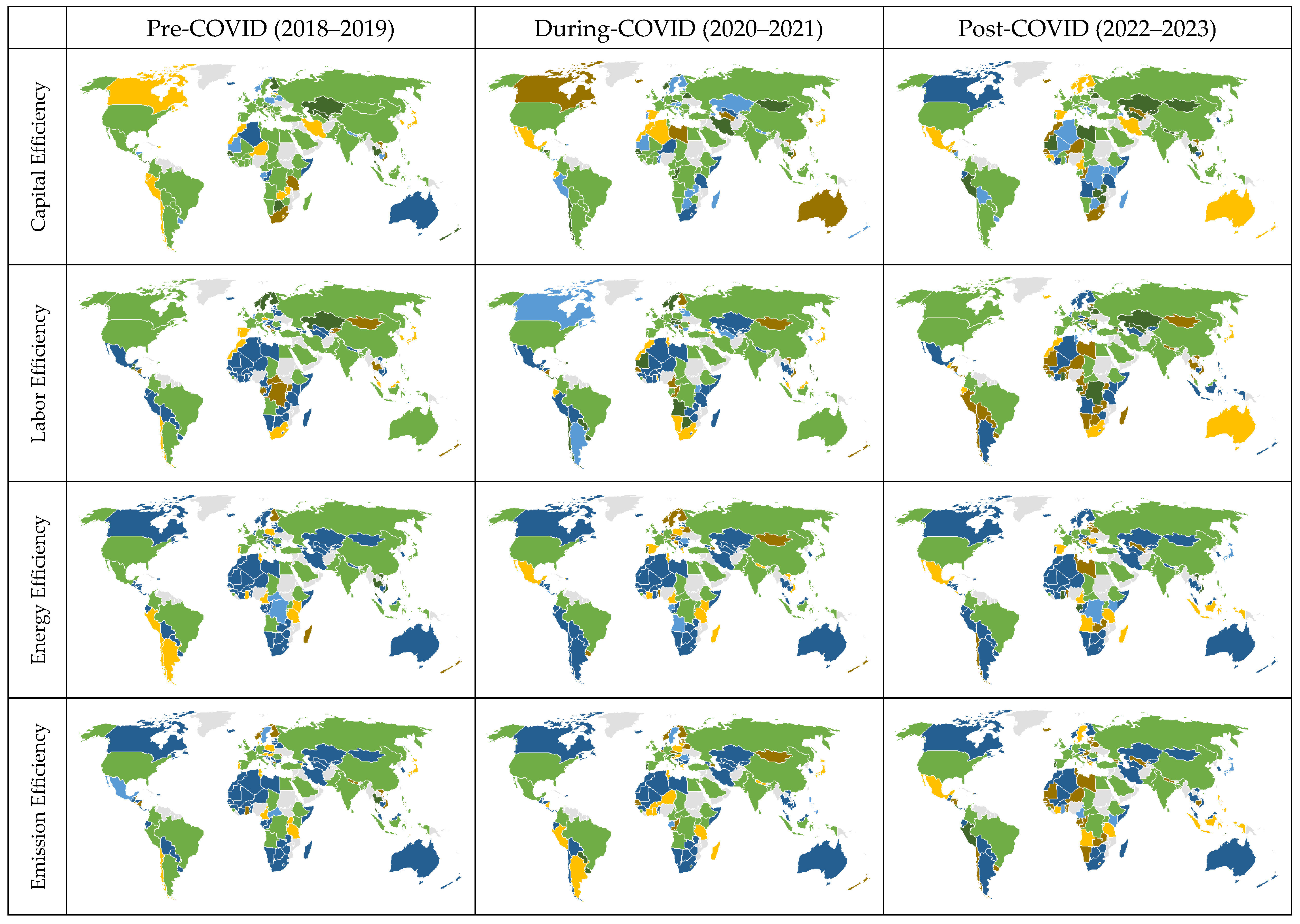
• Capital Efficiency (KE): Measures how close a country’s actual use of gross fixed capital formation (GFCF) is to its optimal frontier target. A higher score indicates that capital is being used with minimal waste.
• Labor Efficiency (LE): Reflects how effectively labor force inputs are transformed into GDP relative to their target values. Countries with low scores use more labor than necessary compared to efficient peers.
• Energy Efficiency (EE): captures how far a country’s energy consumption is from its frontier target, indicating the potential to achieve the same GDP with less energy.
• Carbon Efficiency (CE): indicates the gap between actual CO₂ emissions and the frontier benchmark, showing the extent to which emissions could be reduced without lowering GDP.

The slack values derived from this SBM model are then utilized to calculate key performance indicators (KPIs):

$$CapitalEfficiency\left(KE\right)={\displaystyle \frac{x_{1k}-s_{1k}^{-}}{x_{1k}}}={\displaystyle \frac{x_{1k}^{*}}{x_{1k}}}$$

(2)

$$LaborEfficiency\left(LE\right)={\displaystyle \frac{x_{2k}-s_{2k}^{-}}{x_{2k}}}={\displaystyle \frac{x_{2k}^{*}}{x_{2k}}}$$

(3)

$$EnergyEfficiency\left(EE\right)={\displaystyle \frac{x_{3k}-s_{3k}^{-}}{x_{3k}}}={\displaystyle \frac{x_{3k}^{*}}{x_{3k}}}$$

(4)

$$CarbonEfficiency\left(CE\right)={\displaystyle \frac{y_{1k}^b+s_{1k}^b}{y_{1k}^b}}={\displaystyle \frac{y_{1k}^{b*}}{y_{1k}^b}}$$

(5)

where $x_{1k}^{*}$, $x_{2k}^{*}$, $x_{3k}^{*}$, and $y_{1k}^{b*}$ are target capital, labor force, energy consumption, and CO₂ emission values for the corresponding country. Eco-productivity and eco-efficiency are calculated as follows:

$$Eco-productivity\left(ECOP\right)=KE\times LE$$

(6)

$$Eco-efficiency\left(ECOE\right)=EE\times CE$$

(7)

While all efficiency scores ($KE,LE,EE$, and $CE$) are derived from the same SBM framework and, therefore, reflect interactions among inputs, desirable, and undesirable outputs, we construct two composite indicators for interpretability. Eco-productivity emphasizes the efficiency of transforming traditional productive inputs—capital and labor—into output, whereas eco-efficiency emphasizes environmental performance by combining energy efficiency and carbon efficiency. This separation mirrors the conceptual distinction between factor productivity and environmental efficiency, while maintaining consistency with the slack-adjusted SBM measures.

2.2. Malmquist Productivity Index (MPI) Model

Moving beyond static snapshots of eco-efficiency and sustainable productivity, this section employs the MPI to analyze dynamic changes in eco-productivity over time. MPI decomposes overall productivity change into two key components: efficiency change (EC) and technological change (TC). EC reflects shifts in a country’s distance from the production frontier, capturing whether countries improve their ability to transform inputs into outputs relative to best practices. TC measures the shift of the frontier itself, indicating whether global technological progress is occurring over time. Put simply, EC can be thought of as a country “making better use of its existing resources,” while TC reflects whether the country is “keeping pace with global innovation trends.”

The MPI measures changes in total-factor productivity (TFP) between two periods (e.g., t and t + 1), using DEA-based directional distance functions to assess how far a DMU is from the efficiency frontier. Given the inclusion of CO₂ emissions as an undesirable output, this study employs an MPI formulation that can effectively handle such outputs.

In this study, the MPI is constructed using efficiency scores derived from an SBM-DEA model. Let $D^t\left(x_k,y_k^g,y_k^b\right)$ represent the efficiency score of decision-making unit (DMU) $k$ evaluated against the frontier in period $t$, based on its input $x_k$, desirable outputs $y_k^g$, and undesirable outputs $y_k^b$. Similarly, $D^{t+1}\left(x_k,y_k^g,y_k^b\right)$ is the efficiency of the same DMU when assessed relative to the frontier in period $t+1$. The MPI formulation also requires cross-period or “mixed” efficiency assessments. Specifically, $D^t(x_k^{t+1},y_k^{g,t+1},y_k^{b,t+1})$ evaluates period $t+1$ data using the period $t$ frontier, while $D^{t+1}(x_k^t,y_k^{g,t},y_k^{b,t})$ measures period $t$ data against the period $t+1$ frontier. These four distance functions are then used to compute the MPI and its two components, EC and TC.

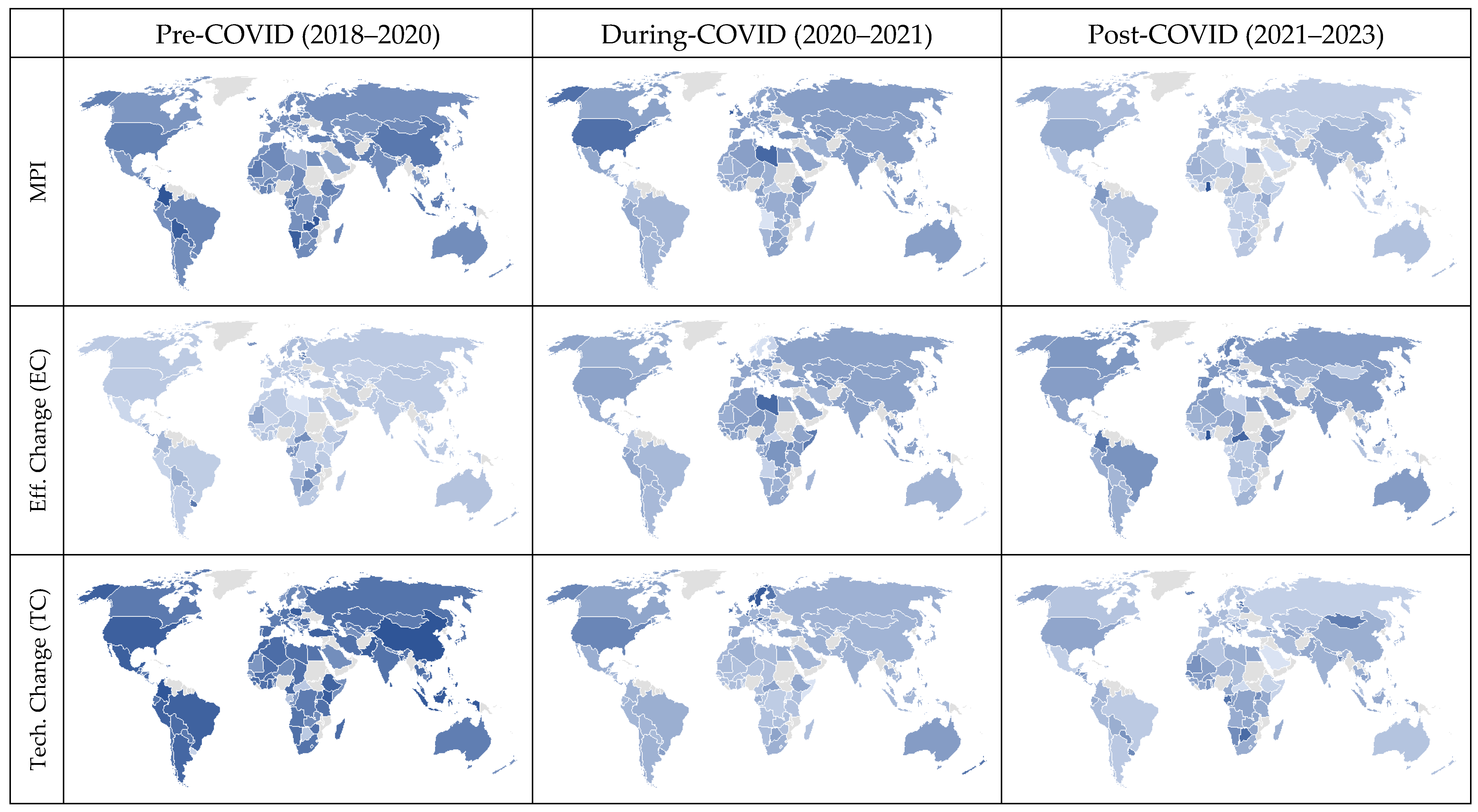
• Efficiency Change (EC): This component, often referred to as the “catch-up” effect, quantifies the change in a DMU’s relative efficiency between periods $t$ and $t+1$. It indicates whether the DMU has moved closer to the efficiency frontier ($EC>1$, an improvement in efficiency), further away ($EC<1$, a deterioration in efficiency), or maintained its relative position ($EC=1$). It is calculated as follows:

  $${EC}_k^{t,t+1}={\displaystyle \frac{D^{t+1}(x_k^{t+1},y_k^{g,t+1},y_k^{b,t+1})}{D^t(x_k^t,y_k^{g,t},y_k^{b,t})}}$$

  (8)
• Technological Change (TC): This component, also known as the “frontier-shift” effect, measures the displacement of the efficiency frontier itself between the two periods. It captures technological progress if the frontier shifts outward ($TC>1$), technological regress if it shifts inward ($TC<1$), or no change in the frontier ($TC=1$). The formula is as follows:

  $${TC}_k^{t,t+1}={\left[{\displaystyle \frac{D^t(x_k^t,y_k^{g,t},y_k^{b,t})}{D^{t+1}(x_k^t,y_k^{g,t},y_k^{b,t})}}\times {\displaystyle \frac{D^t(x_k^{t+1},y_k^{g,t+1},y_k^{b,t+1})}{D^{t+1}(x_k^{t+1},y_k^{g,t+1},y_k^{b,t+1})}}\right]}^{1/2}$$

  (9)

In this study, the MPI is constructed using distance functions derived from the SBM framework, which directly accounts for undesirable outputs. This approach follows the methodology of Tone (2004), ensuring consistency between static (SBM) and dynamic (MPI) analyses. To capture cross-period comparisons, we include “mixed” efficiency terms, where data from period $t+1$ are evaluated against the period $t$ frontier, and, conversely, period $t$ data are evaluated against the period $t+1$ frontier. These cross-period terms allow the MPI to decompose productivity change transparently into $EC$ and $TC$, even when undesirable outputs such as CO₂ emissions are present.

Consequently, the $MPI$ can be expressed as the product of these two components:

$${MPI}_k^{t,t+1}={EC}_k^{t,t+1}\times {{TC}_k^{t,t+1}=\left[{\displaystyle \frac{D^t(x_k^{t+1},y_k^{g,t+1},y_k^{b,t+1})}{D^t(x_k^t,y_k^{g,t},y_k^{b,t})}}\times {\displaystyle \frac{D^{t+1}(x_k^{t+1},y_k^{g,t+1},y_k^{b,t+1})}{D^{t+1}(x_k^t,y_k^{g,t},y_k^{b,t})}}\right]}^{1/2}$$

(10)

An MPI value greater than 1 indicates an improvement in productivity between periods $t$ and $t+1$, whereas a value below 1 signals a decline. By breaking down the index into efficiency and technological components, the decomposition helps determine whether observed productivity changes stem from better resource utilization ($EC$) or from advancements in the production frontier ($TC$). This decomposition is vital, as it distinguishes whether TFP variations stem from enhancements in the utilization of existing technologies (efficiency gains reflected in EC) or from innovations and shifts in the technological frontier itself (advancements reflected in TC). For example, similar TFP growth rates in two nations could hide different underlying realities: one might be rapidly improving its efficiency relative to a static frontier (high EC, low TC), while another might be struggling to adapt to a rapidly advancing global frontier (low EC, high TC). Such distinctions carry different policy implications. The MPI and its constituents will be computed for two key transitional phases: pre-COVID to during-COVID (to capture the pandemic’s initial shock and response) and during-COVID to post-COVID (to assess adaptation and recovery). The necessary distance functions for these MPI calculations will be derived from the SBM-DEA model outputs, ensuring a consistent approach to handling undesirable outputs.

2.3. Sensitivity Analysis of the Model and Variables

To test the robustness of our findings, we conduct a sensitivity analysis along two dimensions. First, we compare results across alternative DEA model specifications—including SBM under both variable returns to scale (VRS) and constant returns to scale (CRS), as well as CCR and BCC models—to examine whether results are sensitive to the choice of returns-to-scale assumption or DEA variant. Second, we examine how efficiency scores change in response to the inclusion or exclusion of key variables, including capital, labor, energy, and CO₂ emissions.

2.3.1. Sensitivity Analysis of the Model

We conduct a comprehensive sensitivity analysis to assess the robustness of the empirical results derived from the primary input-oriented SBM model with VRS. This involves testing the stability of the findings across alternative DEA specifications that differ in orientation and returns-to-scale assumptions—two critical dimensions in DEA modeling. Specifically, we compare results using the CCR and BCC models, as well as the input-oriented SBM model under constant returns to scale (CRS), following the extensions proposed by Sağlam (2017a, 2017b, 2018, 2019) and Demiral and Sağlam (2021, 2023).

• Input-oriented CCR (IO-CCR) Model: DEA is a non-parametric mathematical programming methodology used to assess the relative efficiency of a homogeneous set of DMUs that convert multiple inputs into multiple outputs. The seminal model in this field is the CCR model, introduced by Charnes et al. (1978), which operates under the assumption of constant returns to scale (CRS). The input-oriented CCR model emphasizes input minimization, evaluating the technical efficiency of a DMU by identifying the maximum feasible proportional reduction in its input vector while maintaining its current output levels. This model is particularly suited for settings where inputs can be controlled or reduced, offering a benchmark for identifying inefficiencies and guiding resource optimization. The overall technical efficiency score (${\theta }_k$) of a DMU $k$ is calculated as follows:

  $$\begin{array}{ccc}Min.& {\theta }_k-\epsilon \left({\displaystyle \sum _{r=1}^s}{s}_r^{+}+{\displaystyle \sum _{i=1}^m}{s}_i^{-}\right)& \\ s.t.& {\theta }_k{x}_{ik}-{\displaystyle \sum _{j=1}^n}{x}_{ij}{\lambda }_j-s_{ik}^{-}=0& i=1,\dots ,m;\\ & y_{rk}-{\displaystyle \sum _{j=1}^n}{y}_{rj}{\lambda }_j+s_{rk}^{+}=0& r=1,\dots ,s;\\ & {\lambda }_j,{s_i^{-},s}_r^{+}\ge 0;& j=1,\dots ,n;i=1,\dots ,m;r=1,\dots ,s.\end{array}$$

  (11)
• Input-Oriented BCC (IO-BCC) Model: The input-oriented BCC model, introduced by Banker et al. (1984), is a crucial extension of the original DEA framework that enhances efficiency evaluation by replacing the CRS assumption of the CCR model with the more adaptable VRS. This modification enables the BCC model to differentiate between technical inefficiency and scale inefficiency, providing a more accurate assessment of performance across DMUs operating at various scales. Specifically, the input-oriented BCC model assesses pure technical efficiency (PTE) by determining the maximum proportional reduction in a DMU’s input usage while maintaining its current output levels. It constructs a convex envelopment frontier against which each DMU is benchmarked relative to peers of similar scale. A DMU achieves an efficiency score of one if it operates on this frontier, indicating best-practice performance regardless of any scale-related advantages or disadvantages. The overall PTE score (${\mathsf{\phi }}_{\mathrm{k}}$) of a DMU $k$ is calculated as follows:

  $$\begin{array}{ccc}Min.& {\phi }_k-\epsilon \left({\displaystyle \sum _{r=1}^s}{s}_r^{+}+{\displaystyle \sum _{i=1}^m}{s}_i^{-}\right)& \\ s.t.& {\phi }_k{x}_{ik}-{\displaystyle \sum _{j=1}^n}{x}_{ij}{\lambda }_j-s_{ik}^{-}=0& i=1,\dots ,m;\\ & y_{rk}-{\displaystyle \sum _{j=1}^n}{y}_{rj}{\lambda }_j+s_{rk}^{+}=0& r=1,\dots ,s;\\ & {\displaystyle \sum _{j=1}^n}{\lambda }_j=1& j=1,\dots ,n;\\ & {\lambda }_j,{s_i^{-},s}_r^{+}\ge 0;& j=1,\dots ,n;i=1,\dots ,m;r=1,\dots ,s.\end{array}$$

  (12)
• Input-Oriented SBM (IO-SBM) Model under CRS: The IO-SBM model under CRS, introduced by Tone (2001), is a non-radial DEA approach that provides a more detailed and rigorous assessment of technical efficiency by directly incorporating input slacks. Unlike traditional radial models such as the CCR, which assume proportional input reductions, the IO-SBM model quantifies specific excesses for each input, allowing it to identify inefficiencies that radial models may overlook. Operating under CRS, the IO-SBM model evaluates a DMU’s efficiency relative to a production possibility set that assumes proportional scalability. A DMU is considered fully efficient, with a score of one, only if it exhibits zero slacks across all inputs, indicating that it lies on the efficient frontier with no further potential for non-proportional input reductions. This approach offers a more nuanced and comprehensive measure of inefficiency, making it particularly valuable for performance diagnostics and resource optimization. The IO-SBM model under CRS is formulated as follows for a DMU $\mathit{k}$:

  $$\begin{array}{ccc}Min.& 1-{\displaystyle \frac{1}{m}}{\displaystyle \sum _{i=1}^m}{\displaystyle \frac{s_i^{-}}{x_{ik}}}& \\ s.t.& x_{ik}={\displaystyle \sum _{j=1}^n}{x}_{ij}{\lambda }_j+s_i^{-}& i=1,2,\dots ,m;\\ & y_{r_{1}k}^g={\displaystyle \sum _{j=1}^n}{y}_{r_{1}j}^g{\lambda }_j-s_{r_1}^g& r_1=1,2,\dots ,q_1;\\ & y_{r_{2}k}^b={\displaystyle \sum _{j=1}^n}{y}_{r_{2}j}^b{\lambda }_j+s_{r_2}^b& r_2=1,2,\dots ,q_2;\\ & {\lambda }_j,{s_i^{-},s}_{r_1}^g,s_{r_2}^b\ge 0;& j\in R^n,i\in R^m,r_1\in R^{q_1},r_2\in R^{q_2}\end{array}$$

  (13)

These models offer unique perspectives and computational methods for evaluating efficiency. Utilizing them as robustness checks allows us to determine how independent the results from the primary IO-SBM model are from the model used.

2.3.2. Sensitivity Analysis of the Variables

To evaluate the robustness of the eco-efficiency results and understand the impact of each input variable on the MPI outcomes, we conduct a sensitivity analysis using four alternative model specifications. This analysis examines how the inclusion or exclusion of specific variables affects efficiency scores at the country level, helping to identify the variables that are most significant in determining performance outcomes.

Table 2. Model specifications for sensitivity analysis of the variables.

	Input Variables			Output Variables
	Capital	Labor	Energy	GDP	Emission
Model 1	X	X	X	X	X
Model 2		X	X	X	X
Model 3	X		X	X	X
Model 4	X	X		X	X

presents the four alternative DEA model specifications applied in the variable sensitivity analysis. Model 1 serves as the complete baseline specification, including all three input variables (K, L, and E) and both output variables (GDP and CO₂ emissions). Models 2–4 remove one input variable (K, L, and E) in sequence, to assess its effect on the efficiency scores. This structure facilitates a focused assessment of how country-level efficiency estimates are sensitive to the inclusion of each input variable.

Because this study employs an input-oriented DEA model, our sensitivity checks focus on input variables (capital, labor, and energy). CO₂ is modeled as an undesirable output, and therefore, a “CO₂-free” specification would not be consistent with the orientation of the analysis. This ensures that results remain aligned with the environmental dimension of efficiency.

All computations were conducted in R version 4.3.1, using the DJL package for DEA and MPI estimations. The dataset covers 141 countries observed annually from 2018 to 2023, yielding a balanced panel of 846 country-year observations.

3. Data and Variables

This section details the selection of variables, the data sources, and the temporal scope of the analysis. The construction of the dataset is foundational to the empirical investigation of eco-efficiency and productivity outlined in this study.

Figure 1 illustrates the cumulative growth of key variables worldwide from 1990 to 2023, highlighting distinct trends in economic and environmental performance. While our empirical analysis focuses on 2018–2023, Figure 1 presents long-run (1990–2023) trajectories of the selected variables. This broader perspective demonstrates their strong co-movement and justifies their inclusion in the DEA framework. Against this context, we restrict the analysis to 2018–2023 to capture three distinct phases: pre-COVID stability, pandemic disruption, and post-pandemic recovery. GDP shows the strongest growth, more than doubling over the period, indicating sustained global economic expansion. GFCF closely follows, reflecting consistent investment despite disruptions in 2008 and 2020. CO₂ emissions and energy consumption exhibit moderate growth, with both dipping around 2020 due to the pandemic but rebounding afterward, indicating an ongoing reliance on carbon-intensive energy sources. In contrast, labor force growth is steady but slower, suggesting demographic constraints. Overall, the graph illustrates rising productivity but limited decoupling between economic development and environmental impact.

Table 3. Pearson correlation matrix of input and output variables (1990–2023).

	GFCF	Labor Force	Energy Consumption	GDP
Labor Force	0.984 (0.000)
Energy Consumption	0.980 (0.000)	0.987 (0.000)
GDP	0.993 (0.000)	0.983 (0.000)	0.985 (0.000)
CO2 Emission	0.964 (0.000)	0.977 (0.000)	0.997 (0.000)	0.970 (0.000)

This table reports pairwise correlations among inputs (GFCF, labor force, and energy consumption) and outputs (GDP and CO₂ emissions). All coefficients are statistically significant at the 1% level. High correlations between energy and CO₂ emissions (r = 0.997) and between GFCF and GDP (r = 0.993) underscore the relevance of these variables in the DEA framework.

presents the Pearson correlation matrix for the key input and output variables used in the analysis. All correlation coefficients are statistically significant at the 1% level (p < 0.01), indicating strong linear relationships among the variables.

The correlation between GFCF and GDP is particularly high (r = 0.993), reflecting the central role of capital accumulation in driving economic output. Similarly, the labor force is strongly correlated with both GDP (r = 0.983) and energy consumption (r = 0.987), underscoring the close connection between workforce size, production activity, and energy demand. The strongest correlation is observed between energy consumption and CO₂ emissions (r = 0.997), highlighting the direct link between energy use and environmental impact in predominantly carbon-intensive systems.

The correlation between GDP and CO₂ emissions (r = 0.970) further emphasizes the challenge of achieving economic growth while mitigating environmental externalities. Overall, the results justify the inclusion of these variables in the DEA framework and support their relevance in examining the interplay between productivity and sustainability.

In accordance with the methodology discussed in Section 2, we selected the following variables. The model identifies three inputs: GFCF, labor force, and energy consumption. The primary desirable output is gross domestic product (GDP), while the main undesirable output is carbon dioxide (CO₂) emissions. All variable data were retrieved from the World Bank and EIA databases (K (World Bank, 2024a) and L (World Bank, 2024b) data from the World Bank’s World Development Indicators and energy consumption (EIA, 2024c), GDP (EIA, 2024b), and CO₂ (EIA, 2024a) emissions from the EIA) to ensure consistent units and definitions across countries and years. Capital is measured as gross fixed capital formation (constant 2015 USD, WDI code: NE.GDI.FTOT.KD), and labor as labor force, total (ages 15+, modeled ILO estimate, WDI code: SL.TLF.TOTL.IN). GDP is measured in constant 2015 USD PPP, energy consumption in quadrillion BTU, and CO₂ emissions in million metric tons (MMt). A final balanced sample of 141 countries was constructed by including only those with complete data across all variables for the full period of 2018–2023.

A critical aspect of the research design is the selection of the 2018–2023 period. This timeframe is deliberately chosen to allow for an analysis covering three distinct and significant global economic phases: the pre-COVID period (2018 and 2019), the primary pandemic impact period (2020 and 2021), and the subsequent post-pandemic recovery trajectory (2022 and 2023).

3.1. Input Variables

The input variables used in this study—GFCF, labor force, and energy consumption—capture essential dimensions of national production capacity and resource utilization, especially in light of the unprecedented global disruptions caused by COVID-19. Grounded in the literature on DEA and macroeconomic productivity assessment, these inputs facilitate a nuanced evaluation of country-level efficiency across three distinct phases: the stable pre-pandemic period (2018–2019), the highly disruptive pandemic phase (2020–2021), and the post-pandemic recovery period (2022–2023). This temporal framing is crucial for understanding how capital investment, labor market dynamics, and energy use responded to and evolved in response to the systemic shocks of the COVID-19 crisis.

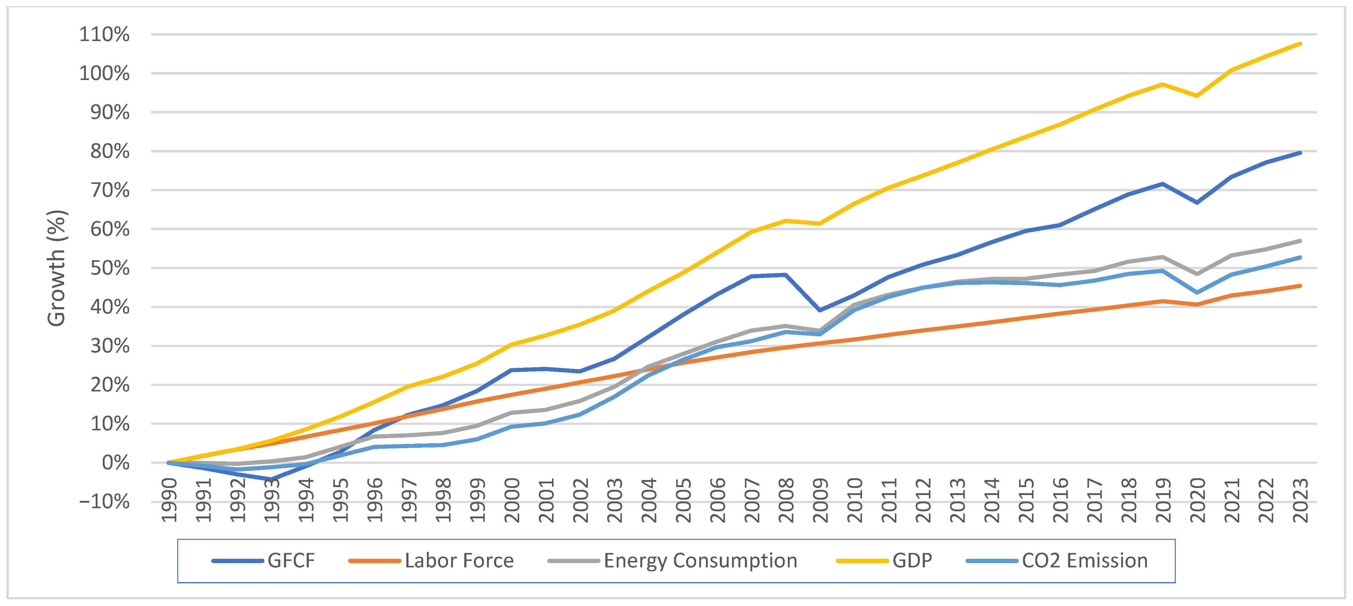
• GFCF reflects country-level investment in physical assets such as infrastructure, machinery, equipment, and facility construction—key drivers of long-term economic growth and technological progress. Between 2018 and 2023, the average GFCF across countries was approximately USD 167.97 billion, with values ranging from USD 134 million to over USD 7.49 trillion, underscoring the wide disparity in investment capacity. As a capital input, GFCF indicates an economy’s capacity to expand its productive frontier. The dataset reveals a significant global contraction in GFCF in 2020, coinciding with the peak of COVID-19-related economic disruptions. The extent of the decline and the subsequent recovery varied considerably across income levels and regions. Advanced and upper-middle-income economies typically experienced a sharp rebound from 2021 onward, supported by large-scale stimulus measures and improved investor confidence. In contrast, many low-income and commodity-dependent countries faced slower recoveries due to limited fiscal capacity and ongoing structural challenges. Understanding these investment patterns is crucial for grasping differences in capital efficiency and the level of economic resilience during recovery.
• Labor force represents the total number of individuals who are either employed or actively seeking work, serving as a proxy for human capital input. Labor force participation reflects not only demographic trends but also institutional factors such as labor regulations, social safety nets, and the adaptability of labor markets. Over the study period, the average labor force size was approximately 23.1 million, with values ranging from 57,484 to over 781 million. The global labor market experienced significant turbulence as a result of the COVID-19 pandemic. In 2020, many countries recorded a decline in labor force size due to pandemic-related shutdowns, mobility restrictions, and health-related absences. While labor force levels began to recover in 2021, the pace and completeness of recovery varied. High-income countries, with robust public health systems and labor protections, generally returned to pre-pandemic levels more quickly. Meanwhile, several developing countries exhibited slower or irregular labor force recovery, impacted by long-term scarring effects and vulnerabilities in the informal sector. These disparities have direct implications for assessing labor productivity and identifying gaps in labor market resilience.
• Energy consumption serves as a vital indicator of an economy’s industrial activity scale, transportation demand, and overall production processes. As a physical input, energy use is closely tied to both output levels and environmental externalities, making it a dual-purpose variable in efficiency and sustainability assessments. The average energy consumption from 2018 to 2023 was 3.84 quadrillion BTU, with minimum and maximum values ranging from 0.0031 to 161.9 quadrillion BTU. The data reveal a sharp decline in energy consumption in 2020 across most countries, driven by widespread lockdowns, reduced economic activity, and supply chain disruptions. The rebound in energy demand from 2021 onward varied by structural characteristics: energy-intensive and export-oriented economies displayed a strong resurgence, while more diversified or energy-efficient countries showed gradual increases in demand. The evolution of energy consumption during this period reflects shifting production patterns and policy choices aimed at balancing recovery with environmental commitments. This variable is particularly relevant for interpreting eco-efficiency and the broader implications of resource use in the post-pandemic recovery landscape.

Together, these inputs form the foundation of our DEA-based evaluation of country-level productivity and efficiency, allowing us to account for diverse pathways of investment, labor mobilization, and resource intensity in a rapidly evolving global context.

3.2. Output Variables

The output variables in this study—gross domestic product (GDP) and carbon dioxide (CO₂) emissions—jointly reflect the dual objectives of economic performance and environmental sustainability. GDP, as a desirable output, captures the overall economic value generated by a country and serves as a benchmark for productivity and growth. In contrast, CO₂ emissions are considered an undesirable output, representing the environmental costs associated with production activities. This dual-output approach aligns with the growing emphasis in the literature on measuring not only the quantity of output but also its quality and sustainability. By incorporating both economic and environmental dimensions, the analysis provides a more comprehensive assessment of efficiency, particularly in light of the COVID-19 pandemic, which altered both output trajectories and environmental externalities across countries between 2018 and 2023.

• Gross domestic product (GDP) serves as the primary measure of economic output in this analysis, capturing the total economic value generated by a country through the production of goods and services. As a widely accepted indicator of economic performance, GDP reflects the productive capacity and market activity that underpin national development. Over the 2018–2023 period, the average GDP between 2018 and 2023 was approximately USD 893 billion, with values ranging from a minimum of USD 0.97 billion to a maximum of USD 27.31 trillion. GDP trends reveal significant disruptions and asymmetries driven by the COVID-19 pandemic. While most countries experienced a sharp contraction in 2020 due to lockdowns, supply chain disruptions, and reduced consumer demand, the scale and pace of recovery in subsequent years varied widely. Advanced economies often showed strong rebounds fueled by fiscal and monetary interventions, whereas many developing countries faced prolonged stagnation or slower growth due to structural constraints. These variations in GDP trajectories are crucial for evaluating changes in output efficiency across different phases of the pandemic and for understanding how national economies responded to post-crisis conditions.
• Carbon dioxide (CO₂) emissions are included as an undesirable output to capture the environmental externalities associated with economic activity and energy use. As a key driver of climate change, CO₂ emissions serve as a critical indicator of the environmental cost of production, making their inclusion essential for evaluating eco-efficiency. Over the 2018–2023 period, the average annual CO₂ emissions across countries were approximately 241 MMt CO₂, with individual country values ranging from 0.22 MMt CO₂ to 12,196 MMt CO₂. CO₂ emission patterns closely mirrored the economic and mobility disruptions brought on by the COVID-19 pandemic. Most countries recorded a noticeable decline in emissions in 2020, reflecting reduced industrial output, transportation activity, and energy consumption during lockdowns. However, emissions rebounded in many economies as restrictions eased and production resumed in 2021 and 2022, although the magnitude of the recovery differed based on the energy structure, policy responses, and decarbonization commitments. By accounting for CO₂ emissions as an undesirable output, this study integrates sustainability into the efficiency framework, enabling a more comprehensive assessment of how countries balanced economic recovery with environmental impact in the post-pandemic period.

In sum, the combined use of GDP and CO₂ emissions as output variables enables a comprehensive evaluation of national performance that accounts for both economic productivity and environmental sustainability. By capturing shifts in output levels and ecological impact across the pre-, during-, and post-COVID periods, this dual-output approach reflects the evolving trade-offs faced by countries as they pursued recovery and growth in a context of global uncertainty. This framework establishes the basis for assessing how effectively nations have transformed inputs into desirable outcomes while mitigating undesirable consequences, offering critical insights into the dynamics of sustainable efficiency in a post-pandemic world. Descriptive statistics for all input and output variables across the 2018–2023 period are reported in

Table 4. Descriptive statistics of input and output variables (2018–2023).

		Input Variables			Desirable Output	Undesirable Output
		GFCF (Billion 2015 USD)	Labor Force (Million People)	Energy Consumption (Quadrillion BTU)	GDP (Billion 2015 USD PPP)	CO2 Emissions (Million Metric Tons)
2018	Mean	152.861	22,590.507	3.769	843.959	240.067
	StDev	636.156	80,741.076	14.597	2622.763	1024.673
	Minimum	0.175	67.026	0.003	1.090	0.278
	Q1	3.594	1591.688	0.093	34.966	5.688
	Median	11.573	4873.299	0.292	119.661	18.872
	Q3	79.912	13,608.204	1.745	543.064	99.522
	Maximum	5953.000	776,868.988	136.574	21,317.630	10,601.870
2019	Mean	156.314	22,831.280	3.819	869.326	242.168
	StDev	656.418	81,070.190	14.922	2732.846	1048.783
	Minimum	0.151	64.684	0.003	1.139	0.220
	Q1	3.636	1606.570	0.097	36.685	5.706
	Median	11.999	4904.458	0.309	123.332	18.999
	Q3	75.446	13,975.088	1.763	554.217	100.040
	Maximum	6115.052	775,928.449	142.096	22,614.990	10,983.970
2020	Mean	152.969	22,606.234	3.656	844.288	228.972
	StDev	664.262	80,247.533	14.704	2719.089	1031.439
	Minimum	0.134	61.844	0.004	1.104	0.261
	Q1	3.373	1578.075	0.092	34.482	5.428
	Median	11.985	4980.288	0.274	107.201	16.887
	Q3	68.574	14,626.913	1.658	529.581	99.023
	Maximum	6240.247	763,830.073	144.442	23,136.770	11,046.936
2021	Mean	175.236	23,154.782	3.833	901.431	239.796
	StDev	769.980	82,261.422	15.442	2921.965	1073.958
	Minimum	0.172	59.595	0.005	1.025	0.303
	Q1	3.902	1612.577	0.095	37.189	5.485
	Median	13.946	4937.106	0.309	120.250	18.450
	Q3	80.236	14,862.735	1.794	564.236	103.444
	Maximum	7475.906	781,187.865	151.637	25,123.270	11,442.165
2022	Mean	181.715	23,525.328	3.900	933.984	245.053
	StDev	794.447	82,511.177	15.661	3013.175	1082.020
	Minimum	0.161	57.627	0.005	0.971	0.305
	Q1	4.197	1621.653	0.099	38.674	5.397
	Median	14.980	5012.404	0.309	130.544	19.318
	Q3	87.636	15,522.682	1.820	589.285	106.559
	Maximum	7493.288	770,113.477	153.520	25,910.600	11,484.335
2023	Mean	188.706	23,909.350	3.983	966.245	250.777
	StDev	805.480	83,816.668	16.237	3150.574	1134.404
	Minimum	0.172	57.484	0.005	1.049	0.313
	Q1	4.445	1634.355	0.101	41.900	5.890
	Median	15.702	5089.291	0.307	133.211	19.203
	Q3	94.166	16,078.729	1.945	604.609	108.603
	Maximum	7356.190	774,607.590	161.897	27,313.920	12,195.657

This table summarizes mean, standard deviation, quartiles, and extreme values for all inputs (GFCF, labor force, and energy consumption) and outputs (GDP and CO₂ emissions) across 141 countries. The wide dispersion across variables highlights cross-country heterogeneity, supporting the use of a VRS framework in DEA.

.

4. Results

4.1. Uneven Efficiency Trajectories in Response to COVID-19: IO-SBM Analysis

To understand how countries’ macroeconomic efficiency evolved in response to the COVID-19 shock, we categorize the sample period into three distinct phases: pre-COVID (2018–2019), COVID (2020–2021), and post-COVID (2022–2023). We compute average input-oriented SBM efficiency scores for each country across these periods and examine both cross-sectional patterns and temporal shifts. The findings offer insights into how effectively countries managed their economic inputs under normal conditions, during a crisis, and throughout the recovery phase.

The results reveal a notable increase in average efficiency during the COVID-19 period (mean = 0.734), up from 0.663 in the pre-COVID years. This improvement may reflect temporary gains driven by emergency policy interventions, targeted resource reallocations, and enhanced operational discipline under crisis conditions. Many governments prioritized essential sectors, curtailed inefficient spending, or restructured operations in ways that boosted short-term input efficiency.

However, the average efficiency declined to 0.675 in the post-COVID phase. This drop is not indicative of a widespread regression. Still, it is instead driven by significant efficiency deteriorations in a subset of countries—particularly Angola, Indonesia, Uruguay, and Gabon—that had previously shown strong pandemic-period performance. Several potential factors may explain these reversals. First, countries heavily reliant on extractive industries or commodity exports (e.g., Angola and Gabon) may have experienced efficiency distortions due to volatile global demand and post-pandemic market realignments. Second, some nations may have benefited from temporary crisis-driven efficiency (e.g., reduced energy use or simplified operations) that proved unsustainable once regular economic activity resumed. Third, countries like Indonesia and Uruguay might have faced fiscal constraints or structural bottlenecks—such as labor market rigidities, weakened institutional capacity, or delayed reforms—that hindered their ability to sustain efficiency gains.

These patterns highlight the risk of treating short-term efficiency improvements during crises as indicative of long-term resilience and underscore the importance of embedding structural reforms into recovery strategies.

A country-level analysis reveals that Gabon (+0.411), Uruguay (+0.363), Slovenia (+0.347), Costa Rica (+0.343), and Brunei (+0.340) experienced the most significant efficiency improvements from pre-COVID to COVID years. These improvements may stem from a mix of factors such as relatively swift and coordinated public health responses (e.g., Uruguay and Slovenia), structural shifts toward lower-emission or knowledge-based sectors (e.g., Costa Rica), commodity-driven economic resilience (e.g., Gabon and Brunei), and effective reallocation of resources under crisis conditions. In some cases, temporary reductions in demand or production may have inadvertently improved input-to-output ratios, particularly in economies with previously high levels of energy or capital intensity. In contrast, countries such as Greece (−0.153), the Philippines (−0.105), Austria (−0.104), Armenia (−0.099), and Sweden (−0.094) experienced marked declines in input efficiency, reflecting their relative vulnerability to economic disruption. These drops may be attributed to a combination of factors, including high dependence on tourism and service sectors (e.g., Greece and Austria), limited fiscal space to absorb shocks (e.g., Armenia and the Philippines), and structural rigidities in labor or energy systems (e.g., Sweden), all of which constrained their ability to maintain productivity under crisis conditions.

In the post-COVID phase, Poland demonstrated the most significant rebound, gaining (+0.183) points and achieving full efficiency. This strong performance likely reflects the effectiveness of fiscal stimulus, EU-supported recovery investments, and Poland’s industrial base benefiting from supply chain realignments. Other notable performers included Ghana (+0.174), Guinea-Bissau (+0.104), Japan (+0.079), and Malaysia (+0.044), suggesting successful structural adjustments, targeted recovery policies, or improved resource allocation following the crisis. For instance, Ghana and Guinea-Bissau may have benefited from the resilience of their agricultural and commodity sectors, while Japan and Malaysia leveraged advanced production systems and recovered external demand.

In contrast, countries like Angola (−0.263) and Indonesia (−0.251), despite strong performance during the pandemic, experienced sharp post-crisis efficiency declines—potentially due to overreliance on temporary gains (e.g., suppressed demand and resource windfalls) that proved unsustainable in recovery. Similar reversals in Uruguay, Gabon, and Namibia suggest that early efficiency improvements may not have been rooted in long-term structural change, highlighting the challenge of maintaining efficiency gains once emergency conditions and policy supports were withdrawn.

Overall, the heterogeneity in efficiency trajectories highlights varied national responses to global shocks and the importance of resilience and long-term institutional capacity in sustaining productivity improvements.

Figure 2 presents the spatial distribution of efficiency group classifications across the pre-COVID, during COVID, and post-COVID periods. Countries are categorized into six groups based on their average efficiency scores and stability (standard deviation) over each two-year window. This visual representation highlights temporal and regional shifts in sustainable productivity performance, revealing how some countries maintained high efficiency under stable conditions, while others experienced greater volatility or persistent inefficiency.

4.2. Cross-Country Dynamics in Sustainability Performance Indicators Across the COVID-19 Period (2018–2023)

Capital Efficiency: An analysis of capital efficiency across 141 countries from 2018 to 2023 highlights a pattern of temporary gains during the pandemic, followed by uneven post-COVID outcomes. While 35 countries registered improvements in capital efficiency between the COVID (2020–2021) and post-COVID (2022–2023) periods, 73 countries experienced declines, indicating that crisis-era capital productivity was often unsustainable without long-term reforms. The strongest post-COVID efficiency gains were observed in Togo (+0.27), Turkmenistan (+0.24), Guinea-Bissau (+0.21), the Czech Republic (+0.19), and Chile (+0.18), potentially reflecting improved capital allocation, public investment strategies, or structural adjustments. In contrast, sharp post-crisis reversals were recorded in Angola (−0.39), Guatemala (−0.34), Côte d’Ivoire (−0.33), Benin (−0.32), and Zimbabwe (−0.28), suggesting fragility in capital utilization and possibly inefficient reinvestment patterns or delayed recovery of capital-intensive sectors. The distribution of countries by post-COVID group classification further underscores this divergence. A total of 63 countries were categorized as Efficient and Stable, indicating sustained high capital productivity with minimal volatility. However, a significant number fell into Moderate and Volatile (25) and Efficient and Volatile (21) groups—highlighting inconsistent performance even among otherwise productive economies. Additionally, 19 countries were classified as either Inefficient and Stable or Inefficient and Volatile, reflecting persistent structural inefficiencies in capital utilization.

These findings suggest that, while some countries succeeded in stabilizing capital efficiency post-pandemic, many others struggled to transition from emergency-driven resource use to long-term productive investment. Policymakers aiming to sustain capital efficiency should focus on improving investment quality, strengthening capital management institutions, and reducing inefficiencies in infrastructure deployment and asset utilization. Without such reforms, the temporary efficiency gains made during crisis conditions risk fading as economies return to normal.

Labor Efficiency: An in-depth analysis of labor efficiency trends across 141 countries from 2018 to 2023 reveals a mixed recovery landscape characterized by significant divergences. While 28 countries achieved gains in labor efficiency between the COVID (2020–2021) and post-COVID (2022–2023) periods, the vast majority—90 countries—experienced declines. This widespread regression indicates that many pandemic-era labor efficiency gains were transitory and not supported by structural improvements. Countries such as Ghana (+0.33), Malaysia (+0.25), Guinea-Bissau (+0.19), Kazakhstan (+0.18), and The Gambia (+0.17) recorded the most significant post-COVID gains, likely due to targeted labor policies, digitalization, and the reallocation of labor to higher-productivity sectors. In contrast, Togo (−0.58), Indonesia (−0.52), the Dominican Republic (−0.47), Uruguay (−0.46), and Belize (−0.45) experienced the steepest declines, reflecting potential challenges in labor reintegration, loss of emergency wage support, or structural weaknesses in their employment systems.

Post-COVID group classifications further highlight this imbalance: 40 countries were categorized as Inefficient and Volatile, while only 39 remained Efficient and Stable. A significant portion also fell into the Inefficient and Stable category (31 countries), with relatively few in the Moderate and Stable (7) or Efficient and Volatile (6) categories. These results emphasize that maintaining labor efficiency in a post-crisis context is more complex than achieving it under emergency constraints. For sustained improvement, countries must move beyond reactive labor measures and adopt forward-looking policies, such as investing in vocational training, reducing labor informality, enhancing social protection systems, and fostering institutional adaptability in labor markets. Without these, labor efficiency is unlikely to stabilize, and crisis-driven productivity gains risk being reversed.

Energy Efficiency: Energy efficiency trends from 2018 to 2023 indicate that most countries faced challenges in maintaining performance after the pandemic. Between the COVID (2020–2021) and post-COVID (2022–2023) periods, only 21 countries improved their energy efficiency, while a significant 100 countries experienced declines. Notable post-COVID winners included Poland (+0.26), Ghana (+0.20), Belize (+0.09), Morocco (+0.08), and Djibouti (+0.08), likely due to energy policy reforms, increased use of renewables, or efficiency gains in energy-intensive sectors. In contrast, Brunei (−0.27), Mongolia (−0.25), Equatorial Guinea (−0.24), Tunisia (−0.23), and Gabon (−0.22) faced the most significant declines, potentially reflecting a return to fossil fuel reliance, inefficient energy subsidies, or inadequate energy governance.

Post-COVID groupings reveal a concentration in Inefficient and Stable (67 countries) and Inefficient and Volatile (19), with only 35 countries maintaining Efficient and Stable performance. These results suggest that the temporary improvements observed during the pandemic—possibly linked to reduced industrial activity and energy consumption—did not translate into lasting structural energy efficiency gains. To reverse these declines, policymakers must invest in clean energy infrastructure, enhance grid efficiency, and decrease reliance on volatile or carbon-intensive energy systems. Long-term efficiency in the energy sector depends not just on technological upgrades but also on institutional reforms that promote sustainable energy planning and pricing.

Emission Efficiency: Between 2018 and 2023, emission efficiency trends indicate a significant post-COVID downturn in most countries. While 18 countries improved their emission efficiency from the COVID-19 period (2020–2021) to the post-COVID-19 period (2022–2023), 100 countries saw declines, highlighting the challenge of maintaining reduced emissions once economic activity returned to normal. Notable post-COVID gainers include Poland (+0.33), Ghana (+0.17), Japan (+0.08), Morocco (+0.05), and Guatemala (+0.04), which may be attributed to energy transition efforts, industrial modernization, or lasting behavioral changes following the pandemic. Conversely, Brunei (−0.30), Indonesia (−0.30), Gabon (−0.28), Lithuania (−0.24), and Georgia (−0.22) experienced the most significant declines in efficiency, which may be linked to a resurgence in carbon-intensive activities or weaker institutional mechanisms for emission management.

Post-COVID group classifications reinforce these findings: 44 countries fell into the “Inefficient and Stable” category, while another 40 were in the “Inefficient and Volatile” category. Only 37 countries maintained efficient and stable emission performance. These patterns suggest that the temporary emission reductions during the COVID-19 pandemic were not structurally embedded and were reversed as mobility, industry, and fossil fuel use returned to pre-pandemic levels. Looking ahead, countries need to implement long-term decarbonization strategies, including carbon pricing, energy diversification, and emissions regulation, to sustain efficiency gains and align economic recovery with climate goals.

Eco-productivity: The analysis of eco-productivity from 2018 to 2023 reveals significant post-pandemic volatility. While only 23 countries improved their eco-productivity in the transition from the COVID period (2020–2021) to the post-COVID period (2022–2023), a striking 99 countries experienced declines. This sharp contrast suggests that many pandemic-era gains were temporary and not structurally embedded. The top post-COVID performers included Ghana (+0.33), Guinea-Bissau (+0.32), Malaysia (+0.22), Tunisia (+0.15), and Japan (+0.14), likely benefiting from targeted sustainability investments, sectoral shifts, or improved input–output coordination. In contrast, Indonesia (−0.52), Uruguay (−0.48), Angola (−0.45), Belize (−0.40), and Uganda (−0.40) saw the steepest declines, indicating challenges in maintaining efficiency gains once emergency conditions subsided.

Post-COVID group classifications further underscore these challenges: 48 countries were categorized as Inefficient and Stable and 37 as Inefficient and Volatile, while only 35 retained an Efficient and Stable status. The small number of countries classified as Moderate and Stable (3) or Efficient and Volatile (4) highlights the rarity of balanced or high-performing yet inconsistent eco-productivity. These findings emphasize that sustained improvements in eco-productivity require more than short-term policy responses. Long-term progress depends on institutional reforms, green infrastructure investment, and integrated economic and environmental planning that aligns recovery efforts with sustainability goals.

Eco-efficiency trends from 2018 to 2023 indicate a noticeable decline in sustainability performance following the pandemic. Between the COVID (2020–2021) and post-COVID (2022–2023) periods, only 19 countries improved their eco-efficiency, while 104 saw declines, suggesting that many environmental productivity gains realized during the pandemic were not sustained. The leading gainers included Poland (+0.51), Ghana (+0.30), Japan (+0.11), Djibouti (+0.09), and Belize (+0.08), likely benefiting from emissions control measures, clean energy transitions, or reduced resource intensity. In contrast, Indonesia (−0.43), Equatorial Guinea (−0.35), Gabon (−0.35), Angola (−0.34), and Denmark (−0.25) experienced the most significant declines, possibly due to post-crisis rebounds in fossil fuel usage or fading momentum in environmental policies.

Post-COVID classifications reveal that 68 countries belong to the Inefficient and Stable group, 30 to the Inefficient and Volatile group, and only 33 countries remain in the Efficient and Stable category. A small number of countries were classified as Moderate and Stable (5), Moderate and Volatile (3), or Efficient and Volatile (2), highlighting the rarity of balanced or high-performing yet unstable eco-efficiency. These findings suggest that most pandemic-era improvements in eco-efficiency were temporary, underscoring the need for long-term, institutionalized sustainability strategies—including carbon pricing, energy diversification, and integrated environmental planning—to achieve sustainable progress.

Figure 3 illustrates the global classification of countries into six performance groups—Efficient and Stable, Efficient and Volatile, Moderate and Stable, Moderate and Volatile, Inefficient and Stable, and Inefficient and Volatile—based on their average efficiency scores and standard deviations. This classification is applied across three distinct periods: pre-COVID (2018–2019), during COVID (2020–2021), and post-COVID (2022–2023). Each map shows changes in efficiency dynamics over time for key performance indicators, including capital, labor, energy, emissions, eco-productivity, and eco-efficiency.

While the KPIs (capital, labor, energy, and emission efficiency) are presented separately for clarity, it is important to recognize their interdependence within the eco-efficiency and eco-productivity framework. For instance, declines in energy or emission efficiency often coincide with weaker eco-productivity outcomes, as lower resource use efficiency constrains the translation of inputs into desirable economic output. Conversely, improvements in labor or capital efficiency can amplify eco-efficiency gains when supported by technological progress or structural reforms. However, all of these measures are calculated as relative efficiency scores—each country’s performance is benchmarked against the best-performing peers rather than against an absolute standard. This means that shifts in one country’s efficiency are inherently tied to changes in others, limiting the feasibility of one-to-one country-level comparisons for every indicator. Instead, the combined analysis underscores how systemic weaknesses in one dimension (e.g., energy efficiency) can contribute to broader stagnation in eco-productivity, particularly in countries facing structural and institutional barriers.

4.3. Temporal Decomposition of Eco-Productivity in the COVID-19 Context: MPI, EC, and TC Results

To assess the dynamics of productivity change over time, we examine MPI trends across three distinct periods: pre-COVID (2018–2020), during COVID (2020–2021), and post-COVID (2021–2023). These intervals correspond to critical phases of macroeconomic disruption and recovery, providing insight into how productivity patterns evolved in response to the global pandemic.

MPI Results: To assess the evolution of productivity over time, we analyze country-level trends in the MPI across three key phases: the pre-COVID period (2018–2020), the COVID period (2020–2021), and the post-COVID recovery (2021–2023). These phases capture the global economy’s transition through stability, disruption, and gradual normalization, offering insights into the drivers of productivity change and resilience.

During the pre-COVID period, the average MPI across countries stood at 1.018, with a standard deviation of 0.091, indicating widespread productivity growth and notable cross-country variation. High-performing economies, such as Ghana, Ireland, Colombia, and the United States, posted MPI values well above 1.00, reflecting dynamic labor markets, strong innovation ecosystems, and sustained investment in both physical and digital infrastructure. Ghana’s exceptional performance (pre-COVID MPI = 1.172) can be attributed to its infrastructure development and the diversification of its economy beyond natural resources. Similarly, the United States maintained robust productivity growth (MPI = 1.110), supported by high R&D intensity and advanced service-sector capabilities. In contrast, countries like Angola and Armenia recorded marginal gains or stagnation, likely due to their greater dependence on resource-based revenues, exposure to external shocks, and limited institutional capacity for implementing structural reforms.

The onset of the COVID-19 pandemic in 2020 marked a sharp inflection point, with the average MPI declining to 0.987 and the standard deviation narrowing slightly to 0.084. This phase was characterized by productivity contractions in most countries due to public health measures, lockdowns, and the collapse of global supply chains. However, the impact was uneven. A small group of economies, including Bangladesh, Ghana, and the United States, sustained positive productivity growth. Bangladesh leveraged its low-cost manufacturing base and digital remittance flows to maintain momentum (MPI = 1.055), while Ghana again performed strongly (MPI = 1.062), benefitting from mobile technology adoption and targeted policy interventions. The United States mitigated productivity losses through a rapid shift to remote work, large-scale fiscal stimulus, and investment in digital infrastructure (MPI = 1.029). In contrast, Angola, Argentina, and Libya experienced steep declines in productivity (e.g., Angola’s MPI fell to 0.709), primarily driven by economic fragility, political volatility, and inadequate healthcare systems. These disparities highlight the importance of pre-existing institutional strength, digital readiness, and policy flexibility in mitigating the impact of global shocks.

In the post-COVID period, spanning 2021–2023, average MPI values returned to 1.000, suggesting that many economies recovered to their baseline productivity levels. The decline in dispersion (SD = 0.081) indicates a more synchronized global recovery, possibly driven by international coordination on vaccination, trade normalization, and fiscal support. Nonetheless, the pace of recovery was mixed. Several emerging and developing economies, such as Vietnam, India, and Bangladesh, experienced renewed productivity gains, reflecting agile supply chain repositioning, demographic advantages, and digital transformation. Ghana once again stood out with a post-COVID average MPI of 1.161, highlighting the role of strategic economic diversification and efficient governance. The United States sustained its strong performance (post-COVID MPI = 1.127), bolstered by continued investments in automation, logistics, and human capital.

Conversely, countries like Saudi Arabia, Comoros, and Congo-Kinshasa struggled to regain productivity momentum, posting MPI values below 1.00 even during the recovery phase. These outcomes likely reflect persistent structural barriers, dependency on oil, slow vaccine rollouts, and limited fiscal space for stimulus policies. Meanwhile, a group of high-income countries—including Australia, Germany, Canada, and Thailand—exhibited remarkable consistency in MPI performance throughout the entire period. Their low productivity volatility (standard deviation < 0.018) highlights the significance of institutional resilience, macroeconomic stability, and early policy coordination in navigating global disruptions.

In summary, while the global economy showed an overall recovery in productivity after the COVID-19 shock, the path and pace of recovery varied significantly across countries. High-performing economies tended to combine adaptive policy responses, innovation capacity, and structural diversification. In contrast, those experiencing persistent volatility often struggled with limited institutional quality and macroeconomic fragility. These results underscore the crucial importance of long-term investments in education, infrastructure, and governance, particularly for emerging and developing economies seeking to narrow the global productivity gap in the post-pandemic era.

EC Results: This section analyzes country-level changes in efficiency using the efficiency change component of the MPI from 2018 to 2023. By disaggregating the results into three phases—pre-COVID, during COVID, and post-COVID—we gain insight into how managerial practices, input–output coordination, and institutional quality contributed to shifts in relative efficiency across time and space.

During the pre-COVID period (2018–2020), the average efficiency change across all countries was 1.065, indicating widespread improvements in resource utilization and operational performance. However, the standard deviation was high (0.214), suggesting significant variation in the efficiency with which countries converted inputs into outputs. Several economies experienced notable efficiency improvements. Specifically, Puerto Rico and the Central African Republic recorded average scores of 1.134 and 1.125, respectively. In Puerto Rico’s case, this likely reflects the implementation of structural reforms and healthcare investments following Hurricane Maria.

Meanwhile, the Central African Republic may have benefited from post-conflict stabilization and aid-driven public sector improvements. Slovenia (1.097) and Timor-Leste (1.085) also demonstrated significant efficiency growth, bolstered by institutional reforms and targeted infrastructure investments. In contrast, countries such as Armenia (0.916), Angola (0.919), and Guinea (0.928) fell behind. Their performance likely reflects inefficiencies in public administration, energy and utility losses, and underinvestment in logistics and workforce skills.

The COVID-19 period (2020–2021) marked a reversal in these trends, with the average efficiency change dropping to 0.974. While the decline was less severe than that in overall productivity, it reflects widespread challenges in managing disrupted supply chains, transitioning to remote work, and addressing healthcare system burdens. Countries varied significantly in their adaptability. For example, Ghana continued to show efficiency improvement (2020–2021 = 1.017), likely due to effective public sector coordination and the use of mobile platforms for health and finance services. On the other hand, countries like Angola and Libya experienced sharp declines in efficiency (e.g., Angola = 0.761), possibly due to state dependency on oil rents, volatility in global commodity markets, and institutional fragility that hampered crisis response.

In the post-COVID recovery period (2021–2023), average efficiency fell further to 0.952, with a standard deviation of 0.120, indicating a slower-than-expected return to pre-pandemic efficiency levels. This phase likely reflects adjustment frictions, restructured labor markets, and the persistence of logistical inefficiencies. Countries such as Timor-Leste, Slovenia, and Ghana maintained relatively high efficiency scores, suggesting resilient institutional capacity and sustained public investment. Conversely, Guinea, El Salvador, and Armenia continued to underperform, with efficiency levels remaining below 0.95, raising concerns about prolonged distortions in their administrative and economic systems. These trends emphasize that recovery is not only a function of aggregate demand but also hinges on operational agility, policy coherence, and efficient governance.

Notably, some countries exhibited exceptional stability across the entire six-year period. For example, Sri Lanka, China, and Saudi Arabia all reported near-zero standard deviations in efficiency change, reflecting consistent internal processes or possibly the influence of central planning and strong policy continuity. In contrast, Puerto Rico (SD = 0.583), Latvia (0.446), and Gabon (0.429) experienced considerable volatility, suggesting inconsistent institutional responses, vulnerability to external shocks, or fluctuating policy implementation.

Overall, the efficiency change trends underscore that productivity resilience is not solely driven by technological progress or capital deepening—it also depends critically on countries’ ability to maintain efficient use of resources under changing circumstances. High-performing countries demonstrated agility in reallocating resources and adapting institutional practices during crisis and recovery, while structural inefficiencies, fragile institutions, or volatile external conditions often constrained laggards.

TC Results: Technological change reflects improvements in the production frontier due to innovation, process upgrades, and the adoption of new technologies. Analyzing the trajectory of this component helps identify which countries expanded their productive capacities over time and how those gains were distributed across the pandemic timeline.

During the pre-COVID years (2018–2019 and 2019–2020), the average technological change score across all countries was 0.979, with a relatively high standard deviation of 0.139. This suggests that, while some countries made early gains in innovation and frontier-shifting technologies, others either stagnated or regressed. Among the top performers, Switzerland, the United States, Bangladesh, Ireland, and Mauritius recorded average technological change values exceeding 1.07. In high-income countries like Switzerland (1.107) and the United States (1.099), this likely reflects investments in advanced manufacturing, AI integration, and digital infrastructure. Meanwhile, Bangladesh’s strong performance (1.091) may be attributed to its rapid growth in ICT services and digital financial tools, which helped modernize traditional sectors. In contrast, several countries—including the Central African Republic (0.917), Somalia (0.918), and Rwanda (0.934)—reported technological regression, potentially due to conflict, underinvestment in infrastructure, and weak innovation ecosystems.

Interestingly, the average rate of technological change increased to 1.024 during the COVID-19 period (2020–2021), despite a global economic slowdown. This counterintuitive finding may reflect an accelerated adoption of digital technologies and technological substitution prompted by the crisis. Businesses and governments worldwide turned to remote work, e-commerce, telemedicine, and contactless services, leading to the rapid digitization of service delivery. Countries that had already established a foundation for digital transformation—such as the United States, Ireland, and Germany—were well positioned to capitalize on this shift. However, the technological gains were not uniform. For instance, economies with underdeveloped digital infrastructure or policy delays in adapting to crisis conditions, such as Saudi Arabia and Comoros, experienced below-average technological change.

In the post-COVID period (2021–2023), technological change continued to rise, with the global average reaching 1.064. This phase appears to have consolidated many of the gains made during the pandemic, as countries embedded digital tools into long-term business practices, education, logistics, and public services. Countries such as Switzerland, Ireland, and Mauritius sustained high scores, reflecting their ability to leverage crisis-induced transitions into permanent technological upgrading. Meanwhile, the gap widened for countries that struggled to institutionalize digital change, particularly those facing ongoing fiscal constraints, political instability, or low broadband penetration rates.

Countries such as Germany, Japan, and Italy demonstrated the most stable technological performance throughout the period, with standard deviations of less than 0.025. This indicates a consistent trajectory of innovation and frontier expansion, likely bolstered by robust industrial research and development (R&D) systems and coordinated innovation policies. Conversely, Latvia, Macau, Cyprus, and Estonia ranked among the most volatile in terms of technological change, suggesting either erratic innovation output or a reactive rather than strategic approach to adopting new technologies.

Overall, the evidence suggests that the pandemic accelerated a global shift in technological capacity; however, the degree to which countries benefited depended on their pre-existing infrastructure, responsiveness in policy, and long-term commitment to digital transformation. Sustained advancements in technology require more than short-term adaptations—they necessitate supportive ecosystems that promote investment in education, innovation policies, regulatory flexibility, and institutional trust.

It should be noted that TC in the MPI–SBM framework measures outward shifts in the production frontier rather than the direct identification of specific technologies. During COVID, these gains often reflected widespread adoption of digital platforms, remote work capabilities, and innovations in health and supply chain systems. Some developing countries, such as Bangladesh, recorded relatively higher TC improvements due to leapfrogging effects, where late adoption of frontier technologies generated proportionally larger efficiency gains compared to already advanced economies. Thus, the observed TC growth should be interpreted as relative technological progress across countries, not as evidence of discrete technological breakthroughs in each case.

Figure 4 illustrates the global evolution of productivity and its components across three key periods—pre-COVID, during COVID, and post-COVID. Notably, MPI values and technological progress (TC) were relatively high across many regions before the pandemic. At the same time, a marked decline in efficiency (EC) is evident during the COVID period, followed by heterogeneous recovery patterns post-2021. These spatial variations highlight the asymmetric economic impact and recovery trajectories, which are shaped by country-specific conditions and policy responses.

It is important to note that both the SBM efficiency scores and the MPI decomposition capture relative performance rather than absolute values. The temporary increase in efficiency observed during the crisis (Section 4.1) reflects countries that reduced inputs more sharply than outputs during lockdowns, thereby moving closer to the efficiency frontier. However, efficiency change (EC) within the MPI framework may still decline if countries subsequently fall behind the shifting frontier as recovery progresses. Similarly, increases in technological change (TC) indicate that the global production frontier has advanced (for example, due to accelerated adoption of digital or energy-efficient practices in certain economies), but eco-productivity scores may still decrease for countries that fail to keep pace with these frontier shifts. These dynamics explain why short-term efficiency gains can coincide with declining EC, and why rising TC may be observed alongside lower eco-productivity, without constituting a contradiction.

4.4. Sensitivity Analysis

This section conducts a thorough sensitivity analysis to assess the robustness of our main findings across two key aspects. Firstly, we investigate if the outcomes regarding sustainable productivity are affected by the selection of DEA model specifications by comparing results from various input-oriented SBM, CCR, and BCC models. Secondly, we assess how country-level efficiency scores respond to changes in the input–output configuration, particularly by considering the inclusion or exclusion of input variables like capital, labor, and energy consumption.

4.4.1. Sensitivity Analysis Results of the Model

We begin by examining the robustness of the IO-SBM model based on the VRS assumption used in our primary analysis. To this end, we compare its outcomes with results from three alternative DEA model specifications: IO-SBM under CRS, IO-CCR, and IO-BCC. These models differ in their assumptions regarding returns to scale and directional orientation, allowing us to assess whether the relative efficiency rankings of 141 countries remain consistent across various methodological frameworks. This comparison serves as a benchmark to evaluate the sensitivity of our results to model specifications and to confirm that the observed efficiency patterns are not merely artifacts of a particular modeling technique.

Table 5. Summary statistics of four DEA models.

Model	Years	Mean	StDev	Minimum	Q1	Median	Q3	Maximum	MPI (2018–2023)
IO-SBM (under VRS)	2018–2019	1.0183	0.0688	0.6055	0.9900	1.0208	1.0503	1.2301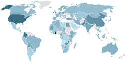
	2019–2020	1.0168	0.1096	0.4944	0.9761	1.0066	1.0460	1.8194
	2020–2021	0.9869	0.0837	0.7091	0.9441	0.9839	1.0128	1.3308
	2021–2022	1.0028	0.0680	0.8288	0.9640	1.0065	1.0434	1.3188
	2022–2023	0.9971	0.0926	0.7897	0.9576	0.9892	1.0186	1.5109
	2018–2023	1.0152	0.1603	0.6602	0.9217	1.0044	1.0801	1.8649
IO-SBM (under CRS)	2018–2019	1.0233	0.0804	0.8653	0.9803	1.0139	1.0532	1.2946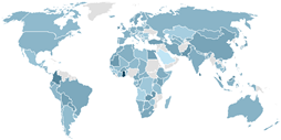
	2019–2020	1.0174	0.0973	0.4920	0.9775	1.0059	1.0574	1.2940
	2020–2021	0.9795	0.0782	0.7241	0.9435	0.9756	1.0057	1.2936
	2021–2022	0.9972	0.0683	0.7006	0.9682	1.0039	1.0405	1.1993
	2022–2023	0.9914	0.1004	0.7526	0.9476	0.9879	1.0134	1.5447
	2018–2023	1.0024	0.1665	0.5342	0.9016	0.9959	1.0608	1.9774
IO-CCR	2018–2019	1.0143	0.0555	0.8440	0.9828	1.0140	1.0407	1.2161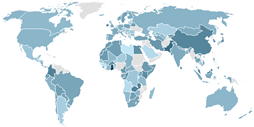
	2019–2020	1.0106	0.0859	0.4997	0.9742	1.0018	1.0474	1.2561
	2020–2021	0.9808	0.0735	0.7953	0.9407	0.9783	1.0098	1.2802
	2021–2022	0.9961	0.0547	0.8336	0.9624	1.0044	1.0370	1.1350
	2022–2023	0.9922	0.0844	0.7451	0.9576	0.9882	1.0161	1.5796
	2018–2023	0.9879	0.1209	0.7031	0.9185	0.9810	1.0487	1.4683
IO-BCC	2018–2019	1.0173	0.0621	0.8332	0.9865	1.0173	1.0355	1.4391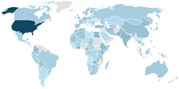
	2019–2020	1.0124	0.0847	0.4928	0.9753	1.0062	1.0562	1.2451
	2020–2021	0.9904	0.0846	0.7870	0.9514	0.9871	1.0171	1.4859
	2021–2022	0.9966	0.0597	0.8157	0.9634	1.0036	1.0371	1.1629
	2022–2023	0.9974	0.0836	0.7967	0.9588	0.9929	1.0208	1.5490
	2018–2023	1.0117	0.1790	0.7030	0.9279	0.9966	1.0658	2.5454

reveals a high level of consistency in central tendencies across the models. The average MPI scores range from 0.988 (IO-CCR) to 1.015 (IO-SBM under CRS), indicating only modest variation in overall productivity levels. However, models that permit greater flexibility in scale assumptions—such as IO-SBM (VRS) and IO-BCC—exhibit higher standard deviations (0.167 and 0.179, respectively), suggesting that these models better capture heterogeneity in country performance. Furthermore, the maximum MPI values differ significantly, with IO-BCC yielding the highest value (2.545), compared to 1.468 for IO-CCR. This indicates that more flexible models are more likely to identify frontier-shifting countries with substantial productivity gains. Despite these variations, the general distribution of MPI scores remains relatively similar, particularly across models, especially for countries consistently near the efficiency frontier.

An analysis of country-level sensitivity to model specification reveals that certain countries exhibit substantial variation in productivity estimates depending on the DEA model used. The United States stands out as the most affected case, with a standard deviation of 0.355 in MPI scores across the four DEA models, suggesting that the choice of returns-to-scale and convexity assumptions significantly influences its assessed productivity change. Ghana and Sri Lanka follow, with standard deviations of 0.267 and 0.238, respectively, indicating considerable model-dependent reclassification. Other countries with notable sensitivity include Bangladesh, Colombia, the United Kingdom, and Saudi Arabia, all of which show meaningful differences in MPI estimates across models. These discrepancies imply that, for certain economies, especially those with complex structures, volatile growth patterns, or unique frontier dynamics, the choice of model specification plays a crucial role in shaping productivity conclusions. Therefore, policy recommendations based on DEA should be made with caution in these contexts, ideally incorporating results from multiple model specifications to ensure robustness and validity.

To evaluate the robustness of country rankings, Spearman rank correlation coefficients were calculated for all model pairs in

Table 6. Spearman rank correlation results of the four DEA models.

	IO-SBM (Under VRS)	IO-SBM (Under CRS)	IO-CCR
IO-SBM (under CRS)	0.902 (0.000)
IO-CCR	0.845 (0.000)	0.908 (0.000)
IO-BCC	0.928 (0.000)	0.841 (0.000)	0.888 (0.000)

. As shown in the table, Spearman rank correlations across the four DEA model specifications are consistently high, providing evidence of robustness across alternative approaches. The results show strong and statistically significant correlations (p < 0.001), ranging from 0.841 to 0.928. The highest rank correlation is found between IO-BCC and IO-SBM (VRS) (ρ = 0.928), reflecting the close alignment in country rankings produced by these two flexible models. Likewise, IO-SBM (CRS) correlates strongly with both IO-SBM (VRS) (ρ = 0.902) and IO-CCR (ρ = 0.908), indicating that country rankings remain relatively stable even as model assumptions about scale change are made. The lowest observed correlation, between IO-BCC and IO-SBM (CRS) (ρ = 0.841), still suggests considerable consistency. Still, it also highlights that the most flexible and most restrictive models may yield slightly divergent assessments for certain countries.

Overall, the findings confirm that the relative rankings of countries are highly robust to model specification, reinforcing the validity of cross-country productivity comparisons. Although absolute MPI scores may shift depending on the model—particularly under VRS—the consistency in rankings suggests that identifying top-performing and underperforming countries is not an artifact of model choice. Nevertheless, the variation in dispersion and extreme values across models also underscores the importance of conducting a sensitivity analysis. Using multiple model specifications offers a more comprehensive and credible assessment of sustainable productivity dynamics across heterogeneous economies.

4.4.2. Sensitivity Analysis of the Input Variables

In this section, we assess the sensitivity of country-level efficiency scores to the inclusion or exclusion of the input variables: capital (K), labor (L), and energy (E) from the baseline model IO-SBM under VRS.

Table 7. Summary statistics of four DEA models for the sensitivity analysis of the input variables.

Model	Years	Mean	StDev	Minimum	Q1	Median	Q3	Maximum	MPI (2018–2023)
Model 1 (IO-SBM)	2018–2019	1.0183	0.0688	0.6055	0.9900	1.0208	1.0503	1.2301
	2019–2020	1.0168	0.1096	0.4944	0.9761	1.0066	1.0460	1.8194
	2020–2021	0.9869	0.0837	0.7091	0.9441	0.9839	1.0128	1.3308
	2021–2022	1.0028	0.0680	0.8288	0.9640	1.0065	1.0434	1.3188
	2022–2023	0.9971	0.0926	0.7897	0.9576	0.9892	1.0186	1.5109
	2018–2023	1.0152	0.1603	0.6602	0.9217	1.0044	1.0801	1.8649
Model 2 (excludes K)	2018–2019	1.0129	0.0840	0.5604	0.9815	1.0134	1.0391	1.5330
	2019–2020	1.0057	0.1287	0.5305	0.9633	0.9927	1.0342	1.9202
	2020–2021	1.0228	0.0956	0.6658	0.9834	1.0236	1.0551	1.4682
	2021–2022	1.0205	0.1082	0.7241	0.9863	1.0218	1.0517	1.7963
	2022–2023	1.0184	0.0848	0.5534	0.9929	1.0157	1.0419	1.6500
	2018–2023	1.0759	0.2024	0.5001	0.9656	1.0500	1.1799	2.0293
Model 3 (excludes L)	2018–2019	1.0251	0.0775	0.8341	0.9871	1.0205	1.0575	1.4740
	2019–2020	1.0324	0.1090	0.4087	0.9840	1.0242	1.0683	1.5289
	2020–2021	0.9747	0.09358	0.6781	0.9292	0.9736	1.0138	1.3620
	2021–2022	1.0029	0.0810	0.6799	0.9520	1.0027	1.0557	1.1772
	2022–2023	1.0021	0.1164	0.7866	0.9566	0.9935	1.0279	2.0336
	2018–2023	1.0329	0.2175	0.6289	0.9060	1.0208	1.1192	2.4739
Model 4 (excludes E)	2018–2019	1.0184	0.0631	0.8013	0.9891	1.0162	1.0414	1.3191
	2019–2020	1.0044	0.0986	0.5300	0.9576	0.9963	1.0463	1.5351
	2020–2021	0.9846	0.0814	0.6635	0.9337	0.9889	1.0205	1.2864
	2021–2022	0.9952	0.0758	0.4922	0.9671	1.0003	1.0372	1.1963
	2022–2023	0.9984	0.1382	0.6498	0.9439	0.9822	1.0168	2.2096
	2018–2023	0.9917	0.1593	0.6051	0.9067	0.9649	1.0558	1.8123

presents the summary statistics for four alternative DEA model specifications used to examine the sensitivity of MPI scores to the selection of input variables. Model 1 represents the baseline input-oriented SBM model, which includes capital, labor, and energy. Models 2–4 sequentially exclude capital (K), labor (L), and energy (E), respectively. The results reveal that excluding key input variables alters both the central tendency and dispersion of productivity estimates. Among the models, Model 3 (which excludes labor) yields the highest average MPI score (1.0329) and the most significant variability (standard deviation = 0.2175), with MPI values reaching a maximum of 2.4739. This indicates that omitting labor significantly inflates productivity estimates and introduces greater heterogeneity across countries. In contrast, Model 4 (which excludes energy) shows the lowest average MPI (0.9917) and moderate variability (standard deviation = 0.1593), suggesting that energy plays a less critical role in driving MPI outcomes. Model 2 (which excludes capital) yields moderately high scores (mean = 1.0759) and dispersion, underscoring the significant role of capital input in shaping efficiency measures.

At the country level, the sensitivity analysis reveals that Ireland, Ghana, and the United States are the most affected by input variable selection, with standard deviations in MPI scores of 0.611, 0.491, and 0.454, respectively, across the four models. Other highly impacted countries include Bangladesh, the United Kingdom, Singapore, and Switzerland, each displaying substantial variation in MPI depending on whether specific inputs are included or excluded. These country-level differences are visualized in Figure 5, which plots MPI trajectories across models for all countries, revealing spikes in divergence, particularly under Models 2 and 3. Overall, the results highlight that model sensitivity is heavily influenced by input selection, with labor and capital having a greater impact on cross-country productivity assessments than energy. Therefore, defining inputs is crucial not only in shaping global averages but also in determining country-specific performance, which necessitates careful consideration in DEA-based policy evaluations.

To statistically evaluate whether input specifications significantly affect MPI outcomes, we applied the Friedman test across the four DEA models used in the sensitivity analysis. As shown in

Table 8. Friedman test results comparing four DEA models for the sensitivity analysis of the input variables.

Models	N	Median	Sum of Ranks
Model 1	141	0.99947	336.0	Null hypothesis: H0: All treatment effects are zero
Model 2	141	1.05860	423.0	Alternative hypothesis: H1: Not all treatment effects are zero
Model 3	141	1.01054	355.0
Model 4	141	0.98046	296.0	DF	Chi-Square	p-Value
Overall	564	1.01227		3	35.92	0.000

, the results indicate significant differences in country-level MPI scores across models (χ² = 35.92, DF 3, p < 0.001). Model 2, which excludes capital, had the highest median score and rank sum, suggesting that capital input plays a substantial role in moderating estimated productivity. Conversely, Model 4, which excludes energy, had the lowest median and rank sum, indicating relatively less sensitivity to the exclusion of energy. These findings align with the descriptive statistics and graphical results presented earlier and confirm that the inclusion or exclusion of key input variables meaningfully alters both the level and distribution of productivity estimates.

The rejection of the null hypothesis indicates that at least one model specification yields significantly different MPI outcomes compared to the others. This reinforces the idea that capital, labor, and energy inputs each capture distinct and essential dimensions of production and sustainability performance. Therefore, all three input variables are necessary for a comprehensive and balanced assessment of eco-efficiency and productivity dynamics across countries. Omitting any of these inputs can bias the results and weaken the reliability of policy-relevant conclusions drawn from the analysis.

4.5. Statistical Analysis

4.5.1. Government Stringency Index (GSI)

The Oxford COVID-19 Government Response Tracker (OxCGRT, Hale et al., 2021) documented government responses to the pandemic from 2020 to 2022. It includes 24 indicators across four categories: Containment and Closure, Economic Support, Health System, and Vaccination. This study utilizes the Stringency Index, which measures the severity of containment and health communication on a scale from 0 to 100 (with 100 representing the strictest measures). The index enables comparisons between countries regarding policy intensity over time. Figure 6 visually presents the global distribution of Stringency Index values for the years 2020 through 2022, highlighting the temporal and cross-country variation in policy responses. The regression analysis examines the relationship between government policy stringency and total-factor productivity growth (TFP) among 141 countries from 2021 to 2023.

The regression analyses provide nuanced insights into the impact of government stringency measures on productivity growth during and after the COVID-19 pandemic. As shown in

Table 9. Impact of Government Stringency Index (GSI) on MPI results (2021–2023 and 2022–2023).

${\mathit{M}\mathit{P}\mathit{I}}_{21-23}=\mathit{\alpha }+{\mathit{\beta }}_1\cdot {\mathit{G}\mathit{S}\mathit{I}}_{2020}+{\mathit{\beta }}_2\cdot {\mathit{G}\mathit{S}\mathit{I}}_{2021}+{\mathit{\beta }}_3\cdot {\mathit{G}\mathit{S}\mathit{I}}_{2022}+\mathit{ϵ}$						${\mathit{M}\mathit{P}\mathit{I}}_{22-23}=\mathit{\alpha }+{\mathit{\beta }}_1\cdot {\mathit{G}\mathit{S}\mathit{I}}_{2020}+{\mathit{\beta }}_2\cdot {\mathit{G}\mathit{S}\mathit{I}}_{2021}+{\mathit{\beta }}_3\cdot {\mathit{G}\mathit{S}\mathit{I}}_{2022}+\mathit{ϵ}$
Term	Coef	SE Coef	T-Value	p-Value	VIF	Term	Coef	SE Coef	T-Value	p-Value	VIF
Constant	1.0077	0.0460	21.91	0.000		Constant	0.9982	0.0370	27.00	0.000
GSI2020	−0.0006	0.0012	−0.53	0.598	1.88	GSI2020	−0.0001	0.0009	−0.11	0.911	1.88
GSI2021	−0.0007	0.0010	−0.68	0.498	2.04	GSI2021	−0.0013	0.0008	−1.61	0.110	2.04
GSI2022	0.0026	0.0010	2.63	0.010	1.20	GSI2022	0.0030	0.0008	3.86	0.000	1.20

, stringency in 2022 proves to be a consistently significant and positive predictor of productivity growth, both in the 2021–2023 and 2022–2023 periods. In the second regression, the 2022 index demonstrates a more substantial effect (coefficient = 0.0030, p < 0.001), reinforcing the notion that later-stage interventions were more effective in supporting economic recovery. In contrast, the stringency measures from 2020 and 2021 exhibit negative coefficients and remain statistically insignificant across both models, suggesting that early and mid-pandemic restrictions may have hindered productivity without yielding long-term economic benefits. All variance inflation factors (VIFs) are below the standard threshold, indicating no concern about multicollinearity. These findings emphasize the importance of adaptive policy design, while initial lockdowns may have been essential for immediate crisis containment. It was the strategic and refined measures instituted in 2022 that appear to have had a positive impact on productivity. Policymakers should, therefore, prioritize evidence-based, targeted interventions during extended crises, focusing on minimizing economic disruptions while maintaining resilience and recovery capacity.

4.5.2. Non-Parametric Tests for World Bank Income Groups and Efficiency Scores

To assess whether eco-efficiency and productivity outcomes vary systematically across different stages of economic development, we conduct non-parametric statistical tests using the World Bank’s income classification system. Countries in the sample are categorized into four groups—low-income, lower-middle-income, upper-middle-income, and high-income—based on gross national income per capita. Given the non-normal distribution and ordinal nature of several eco-efficiency indicators, the Kruskal–Wallis test is first employed to detect overall differences across income groups. To further investigate which specific income groups differ significantly, we conduct a total of 60 pairwise Mann–Whitney U tests across ten performance indicators.

Table 10. Pairwise Mann–Whitney U Test results for eco-efficiency and productivity indicators by income group.

Efficiency	Group 1	Group 2	U-Statistic	p-Value
AVG IO-SBM	Lower-middle-income countries	High-income countries	668.5	0.0765
AVG LE	Upper-middle-income countries	Lower-middle-income countries	987	0.0025
AVG LE	Upper-middle-income countries	High-income countries	725	0.0724
AVG LE	Lower-middle-income countries	High-income countries	438	0.0001
AVG LE	High-income countries	Low-income countries	519	0.0984
AVG EE	Upper-middle-income countries	Low-income countries	167	0.0035
AVG EE	Lower-middle-income countries	Low-income countries	206	0.0571
AVG EE	High-income countries	Low-income countries	271	0.0413
AVG CDE	Upper-middle-income countries	Low-income countries	178	0.0064
AVG CDE	Lower-middle-income countries	Low-income countries	204.5	0.0535
AVG ECOP	Upper-middle-income countries	Lower-middle-income countries	994	0.0020
AVG ECOP	Lower-middle-income countries	High-income countries	449	0.0002
AVG ECOE	Upper-middle-income countries	Low-income countries	171	0.0043
AVG ECOE	Lower-middle-income countries	Low-income countries	209	0.0653
AVG ECOE	High-income countries	Low-income countries	288	0.0741
AVG MPI	Lower-middle-income countries	Low-income countries	404	0.0632
AVG MPI	High-income countries	Low-income countries	572	0.0147
AVG EC	Upper-middle-income countries	High-income countries	576.5	0.0022
AVG EC	Lower-middle-income countries	High-income countries	558	0.0056
AVG TC	Upper-middle-income countries	Low-income countries	519	0.0009
AVG TC	Lower-middle-income countries	Low-income countries	465	0.0025
AVG TC	High-income countries	Low-income countries	569	0.0166

summarizes the subset of significant pairwise differences identified through Mann–Whitney U tests. This approach enables robust comparisons without relying on parametric assumptions, providing policy-relevant insights into the relationship between income level and national environmental-economic performance.

The pairwise Mann–Whitney U test results offer clear evidence that eco-efficiency and productivity performance vary significantly across income levels, with the most significant disparities observed between lower-middle- or low-income countries and their upper-middle- and high-income counterparts. Multiple indicators exhibit statistically significant differences at the 10% level, suggesting that income level plays a central role in shaping environmental and economic efficiency outcomes.

Average labor efficiency (AVG LE) shows particularly sharp contrasts. Upper-middle-income countries outperform lower-middle-income countries (p = 0.0025), and lower-middle-income economies trail significantly behind high-income countries (p = 0.0001). These differences likely reflect variations in capital accumulation, workforce education levels, labor market institutions, and access to automation and digital infrastructure. Policy efforts aimed at boosting labor productivity in lower-income countries may thus require comprehensive investment in workforce development, education, and industrial upgrading.

Similarly, average energy efficiency (AVG EE) and CO₂ emission efficiency (AVG CDE) are markedly higher in upper-middle- and high-income countries compared to low-income countries (p = 0.0035 and p = 0.0064, respectively). These disparities highlight the limited access of low-income countries to clean energy technologies, modern energy grids, and pollution control systems. Development strategies for these countries should prioritize international support for renewable energy deployment, energy infrastructure investment, and technology transfer, particularly through global mechanisms such as the UNFCCC Technology Mechanism or the Green Climate Fund.

Eco-productivity metrics, such as AVG ECOP and AVG ECOE, also reveal significant efficiency gaps across income groups. For example, lower-middle-income countries are significantly less eco-productive than both upper-middle (p = 0.0020) and high-income countries (p = 0.0002). This suggests that economic growth in lower-income settings often comes at a greater environmental cost due to reliance on resource- and emissions-intensive processes. Policies that promote circular economy practices, green supply chains, and low-carbon innovation can help decouple economic activity from environmental degradation.

In addition, technological change (AVG TC)—a proxy for innovation-driven efficiency gains—also differs significantly between low-income countries and all other groups. Upper-middle (p = 0.0009), lower-middle (p = 0.0025), and high-income countries (p = 0.0166) exhibit greater technological progress, indicating a widening innovation gap. Bridging this divide will require policies that strengthen national innovation systems, promote research and development (R&D), and improve the diffusion of clean technologies through regional and global cooperation.

Taken together, these findings suggest that closing the eco-efficiency gap between income groups requires targeted, multi-level policy interventions. In lower-income countries, improving basic infrastructure, enhancing institutional capacity, and enabling access to clean technologies are foundational steps. At the same time, international cooperation—via climate finance, technology partnerships, and development aid—must play a central role in accelerating eco-efficient growth where domestic fiscal space is constrained.

5. Discussions

This study provides a comprehensive overview of how national eco-efficiency and eco-productivity evolved during the COVID-19 crisis and its aftermath. Our results contribute to the growing literature on eco-efficiency and eco-productivity under crisis conditions. Prior macro-level DEA studies, such as Sağlam (2025), showed that productivity in OECD countries declined during COVID-19 but recovered mainly through technological progress rather than efficiency gains. Our broader sample of 141 countries confirms these dynamics while extending the analysis to eco-efficiency and eco-productivity dimensions, thereby highlighting how energy and carbon efficiency drive much of the volatility.

The findings reveal a pattern of temporary gains during the height of the pandemic—particularly in capital and energy efficiency—followed by post-COVID reversals across a subset of countries rather than universally. In line with Reviewer 3, we specify that the decline was concentrated in commodity-dependent economies such as Angola, Indonesia, and Uruguay, rather than a “widespread” pattern. This is consistent with the literature on crisis-driven productivity (e.g., Hsieh & Klenow, 2018), which emphasizes that shocks may generate short-term efficiency spikes that dissipate once normal activity resumes. For policymakers, this highlights the critical importance of embedding long-term institutional and structural reforms rather than relying on emergency-driven performance spikes. As emphasized in Camanho et al. (2024), crisis-induced efficiency gains should be interpreted as fragile, reflecting temporary reallocations rather than structural improvement.

A particularly concerning trend is the sharp post-pandemic decline in labor and energy efficiency across a majority of countries. The inability to maintain labor productivity gains suggests systemic weaknesses in employment institutions, informality, and skill mismatches that were exposed once wage subsidies and crisis-era support mechanisms were lifted. This aligns with studies linking informality and weak labor protections to fragile productivity recoveries in developing countries (Loayza, 2018). Addressing this requires a strategic shift from temporary labor market interventions toward forward-looking workforce development policies. To address this, governments must invest in vocational education, reskilling programs, and digital inclusion to enhance the adaptability of labor markets. In parallel, energy efficiency deteriorated in over 100 countries after 2021, reflecting a return to carbon-intensive practices. This suggests that green gains made during the pandemic—often due to reduced industrial activity—were not structurally embedded. To counter this, national energy policies should prioritize the expansion of renewable energy infrastructure, grid modernization, and energy governance reforms that reward sustainable practices and penalize inefficiency.

While technological progress (as measured by TC) continued even during the most disruptive periods, most countries failed to translate these advancements into operational efficiency. This gap between innovation and implementation—where EC declined while TC improved—indicates that many countries adopted or accessed new technologies but lacked the institutional capacity to fully integrate them. Simply put, frontier technologies alone do not guarantee productivity improvements unless they are supported by responsive institutions, skilled labor, and effective public–private collaboration. This echoes the concept of absorptive capacity, which stresses that frontier technologies alone do not guarantee productivity improvements unless supported by responsive institutions and skilled labor (Cohen & Levinthal, 1990). The results extend this theoretical framework to a global shock, showing that countries with higher institutional quality (e.g., Japan) were better able to convert TC gains into lasting productivity improvements. Therefore, policies that support innovation ecosystems must be accompanied by parallel efforts to enhance absorptive capacity through regulatory reforms, capacity-building in public administration, and targeted incentives for firm-level technology adoption.

Another central insight of this study is the differential effect of government responses depending on timing. While early lockdowns in 2020 and 2021 showed no significant association with productivity growth, the 2022 stringency measures had a positive and statistically significant effect. This may reflect several mechanisms, including higher vaccination coverage, population adaptation to restrictions, and the ability of governments to design more targeted interventions by 2022. This suggests that adaptive, well-calibrated policy interventions—those that evolved in response to the crisis rather than being applied uniformly—were more effective in supporting economic recovery. Governments should institutionalize policy agility by strengthening data-driven decision systems, scenario planning, and real-time feedback loops during crises. The effectiveness of later-stage interventions in 2022 underscores that economic resilience hinges not only on the strength of the response but also on its timing, coherence, and alignment with national development capacities.

Income-level disparities in eco-efficiency and eco-productivity were stark and statistically significant. Low- and lower-middle-income countries have consistently lagged behind in labor, energy, and emission efficiency, as well as in technological advancements. These patterns suggest limited access to clean technologies, inadequate infrastructure, and fiscal constraints. Consistent with the concept of “structural traps” (Rodrik, 2016), these economies face deep institutional and financial barriers that constrain their ability to translate technological opportunities into productivity gains. Narrowing this gap demands targeted international support through concessional climate finance, technology transfer, and capacity-building initiatives. National governments in these regions should also focus on foundational improvements, such as expanding access to clean energy, formalizing labor markets, and strengthening governance frameworks that can channel investments toward sustainable development. For global institutions and development agencies, these findings reaffirm the need to tailor support to structural realities, enabling inclusive transitions toward low-carbon and high-productivity economies.

The classification of countries by efficiency and volatility further highlights the importance of stability, not just high performance. Countries such as Poland, Ghana, and Japan, which maintained or improved efficiency during the recovery phase, did so through coordinated policy strategies, industrial resilience, and sustained public investment. In contrast, countries that exhibited volatility—despite temporary high scores—struggled to lock in gains, often due to over-reliance on commodity cycles, fragmented policy responses, or weak institutional frameworks. Moving forward, economic resilience should be conceptualized as both the level and consistency of performance. Fiscal rules, institutional continuity, and cross-sectoral coordination mechanisms are crucial for reducing volatility and embedding long-term gains. This supports earlier findings that macroeconomic volatility undermines sustainability transitions (Aghion et al., 2021). Countries that institutionalize high-performing and stable eco-efficiency systems will be better positioned to withstand future shocks, including those stemming from climate change and geopolitical disruptions.

Our results are consistent with recent macroeconomic DEA research. Sağlam (2025) showed that productivity in OECD countries declined during COVID-19 but recovered mainly through technological progress rather than efficiency gains. Our broader sample of 141 countries confirms this pattern while extending the analysis to eco-efficiency and eco-productivity dimensions. By distinguishing capital, labor, energy, and carbon efficiency, we further demonstrate that energy and carbon efficiency are the most volatile components, while capital and labor efficiency are more stable but slower to recover. This highlights the need to integrate environmental sustainability into productivity strategies to avoid unsustainable rebounds.

Limitations must also be acknowledged. First, our measure of environmental externalities is limited to CO₂ emissions, excluding other pollutants or biodiversity impacts. Second, while DEA-SBM and MPI allow nuanced efficiency assessments, they remain relative measures and do not establish causal relationships. Third, data availability during 2018–2023 for 141 countries constrained variable selection and may underrepresent fragile states. Finally, pandemic conditions introduced structural breaks that complicate long-term inference. These limitations should be considered when interpreting our findings. These limitations align with concerns raised in Zhou et al. (2010) and Lin and Du (2015), who highlight the sensitivity of MPI results to model specification and pollutant selection.

Overall, the findings highlight that, while technological innovation and emergency policies matter, sustainable eco-productivity depends critically on the long-term capacity of national systems to integrate reforms, build resilience, and institutionalize performance. Policymakers should view the post-pandemic transition not simply as a return to pre-crisis norms but as an opportunity to reconfigure economies around stability, inclusivity, and sustainability.

6. Conclusions

This study presents a comprehensive global analysis of eco-efficiency and eco-productivity dynamics across 141 countries from 2018 to 2023, encompassing the pre-COVID, pandemic, and post-pandemic recovery periods. Using an SBM-DEA framework and Malmquist Productivity Index decomposition, the results highlight the complex interplay between temporary efficiency gains, long-term structural constraints, and varied national responses to one of the most disruptive global shocks in recent history.

While many countries experienced improvements in capital, energy, or emission efficiency during the pandemic, these gains were largely transitory. The post-COVID period was marked by significant declines in commodity-dependent countries rather than universally “widespread” reversals, especially in labor and energy efficiency, underscoring the limits of crisis-driven gains that are not rooted in institutional or structural transformation. Technological progress continued across most regions, yet these advances often failed to translate into operational efficiency due to limited absorptive capacity. The divergence between technological change and efficiency change reveals a key vulnerability in many national systems: innovation without the institutional infrastructure to support its integration delivers limited productivity benefits.

Notably, this analysis reveals that the timing and design of government responses are crucial. While early-stage lockdowns did not significantly contribute to productivity outcomes, adaptive restrictions in 2022, supported by higher vaccination rates and targeted fiscal supports, were associated with positive productivity recovery. This emphasizes the value of responsive and flexible governance during prolonged crises. Income-based disparities further highlight that lower-income countries face systemic disadvantages in eco-efficiency, driven by weaker institutions, technological gaps, and limited access to sustainable infrastructure.

These findings offer several policy lessons. First, countries must transition from emergency responses to long-term reforms that institutionalize efficiency and effectiveness. Investments in labor upskilling, energy system modernization, and governance capacity are crucial for stabilizing and sustaining eco-productivity. Second, innovation policy should be aligned with efforts to strengthen implementation systems—from regulatory coherence to workforce adaptability—to ensure that technological change yields measurable productivity improvements. Third, governments must develop the ability to respond to shocks with agility and precision. Evidence-based, time-sensitive interventions are far more effective than prolonged restrictions or one-size-fits-all solutions. Finally, international cooperation must be intensified to help lower-income countries close the eco-efficiency gap through concessional finance, technology transfer, and targeted institutional support. For instance, technology transfer in renewables can accelerate lower-income growth, while institutional reforms such as carbon pricing remain critical for high-income economies.

Building on the findings of this study, future research could explore several promising directions. First, incorporating additional environmental indicators—such as air quality, biodiversity, or material circularity—would enable a more comprehensive assessment of sustainability beyond carbon efficiency. Second, extending the analysis to subnational units or specific sectors (e.g., manufacturing, agriculture, or transport) could reveal significant within-country disparities and policy-relevant insights at a more granular level. Third, integrating panel data econometric techniques alongside DEA could help disentangle causal mechanisms behind observed efficiency trends, particularly the role of institutional quality, governance structures, and targeted climate policies. Additionally, future studies could investigate how climate-related risks and adaptation strategies impact long-term eco-productivity, particularly in climate-vulnerable regions. Finally, a comparative analysis of post-pandemic stimulus packages and their environmental impacts could shed light on the effectiveness of green recovery strategies across different political and economic systems.

References

- Aghion, P., Antonin, C., & Bunel, S. (2021). The power of creative destruction: Economic upheaval and the wealth of nations. Harvard University Press. [Google Scholar]
- Apergis, N., Aye, G. C., Barros, C. P., Gupta, R., & Wanke, P. (2015). Energy efficiency of selected OECD countries: A slacks based model with undesirable outputs. Energy Economics, 51, 45–53. [Google Scholar] [CrossRef]
- Banker, R. D., Charnes, A., & Cooper, W. W. (1984). Some models for estimating technical and scale inefficiencies in data envelopment analysis. Management Science, 30(9), 1078–1092. [Google Scholar] [CrossRef]
- Brockett, P. L., Golany, B., & Li, S. (1999). Analysis of intertemporal efficiency trends using rank statistics with an application evaluating the macro economic performance of OECD nations. Journal of Productivity Analysis, 11, 169–182. [Google Scholar] [CrossRef]
- Camanho, A. S., Silva, M. C., Piran, F. S., & Lacerda, D. P. (2024). A literature review of economic efficiency assessments using Data Envelopment Analysis. European Journal of Operational Research, 315(1), 1–18. [Google Scholar] [CrossRef]
- Chang, T. P., & Hu, J. L. (2010). Total-factor energy productivity growth, technical progress, and efficiency change: An empirical study of China. Applied Energy, 87(10), 3262–3270. [Google Scholar] [CrossRef]
- Charnes, A., Cooper, W. W., & Rhodes, E. (1978). Measuring the efficiency of decision making units. European Journal of Operational Research, 2(6), 429–444. [Google Scholar] [CrossRef]
- Chien, T., & Hu, J. L. (2007). Renewable energy and macroeconomic efficiency of OECD and non-OECD economies. Energy Policy, 35(7), 3606–3615. [Google Scholar] [CrossRef]
- Choi, Y., Zhang, N., & Zhou, P. (2012). Efficiency and abatement costs of energy-related CO2 emissions in China: A slacks-based efficiency measure. Applied Energy, 98, 198–208. [Google Scholar] [CrossRef]
- Cohen, W. M., & Levinthal, D. A. (1990). Absorptive capacity: A new perspective on learning and innovation. Administrative Science Quarterly, 35(1), 128–152. [Google Scholar] [CrossRef]
- Deliktas, E., & Balcilar, M. (2005). A comparative analysis of productivity growth, catch-up, and convergence in transition economies. Emerging Markets Finance and Trade, 41(1), 6–28. [Google Scholar] [CrossRef]
- Demiral, E. E., & Sağlam, Ü. (2021). Eco-efficiency and Eco-productivity assessments of the states in the United States: A two-stage Non-parametric analysis. Applied Energy, 303, 117649. [Google Scholar] [CrossRef]
- Demiral, E. E., & Sağlam, Ü. (2023). Sustainable production assessment of the 50 US states. Journal of Cleaner Production, 419, 138086. [Google Scholar] [CrossRef]
- Färe, R., Grosskopf, S., Norris, M., & Zhang, Z. (1994). Productivity growth, technical progress, and efficiency change in industrialized countries. The American Economic Review, 84(1), 66–83. [Google Scholar]
- Forstner, H., & Isaksson, A. (2002). Productivity, technology, and efficiency: An analysis of the world technology Frontier; when memory is infinite. Statistics and Information Networks Branch of UNIDO. [Google Scholar]
- Hale, T., Angrist, N., Goldszmidt, R., Kira, B., Petherick, A., Phillips, T., Webster, S., Cameron-Blake, E., Hallas, L., Majumdar, S., & Tatlow, H. (2021). A global panel database of pandemic policies (Oxford COVID-19 Government Response Tracker). Nature Human Behaviour, 5(4), 529–538. [Google Scholar] [CrossRef]
- Hsieh, C. T., & Klenow, P. J. (2018). The reallocation myth. Center for Economic Studies Working Paper, 18, 1–25. [Google Scholar]
- Hu, J. L., & Kao, C. H. (2007). Efficient energy-saving targets for APEC economies. Energy Policy, 35(1), 373–382. [Google Scholar] [CrossRef]
- Hu, J. L., & Wang, S. C. (2006). Total-factor energy efficiency of regions in China. Energy Policy, 34(17), 3206–3217. [Google Scholar] [CrossRef]
- Iftikhar, Y., He, W., & Wang, Z. (2016). Energy and CO2 emissions efficiency of major economies: A non-parametric analysis. Journal of Cleaner Production, 139, 779–787. [Google Scholar] [CrossRef]
- Kaüger, J. J., Cantner, U., & Hanusch, H. (2000). Total factor productivity, the East Asian miracle, and the world production frontier. Weltwirtschaftliches Archiv, 136(1), 111–136. [Google Scholar] [CrossRef]
- Lin, B., & Du, K. (2015). Modeling the dynamics of carbon emission performance in China: A parametric Malmquist index approach. Energy Economics, 49, 550–557. [Google Scholar] [CrossRef]
- Loayza, N. (2018). Informality: Why is it so widespread and how can it be reduced? World Bank research and policy briefs No. 133110. Available online: https://ssrn.com/abstract=3360124 (accessed on 1 July 2025).
- Moutinho, V., Fuinhas, J. A., Marques, A. C., & Santiago, R. (2018). Assessing eco-efficiency through the DEA analysis and decoupling index in the Latin America countries. Journal of Cleaner Production, 205, 512–524. [Google Scholar] [CrossRef]
- Moutinho, V., Madaleno, M., & Robaina, M. (2017). The economic and environmental efficiency assessment in EU cross-country: Evidence from DEA and quantile regression approach. Ecological Indicators, 78, 85–97. [Google Scholar] [CrossRef]
- Park, Y. S., Lim, S. H., Egilmez, G., & Szmerekovsky, J. (2018). Environmental efficiency assessment of US transport sector: A slack-based data envelopment analysis approach. Transportation Research Part D: Transport and Environment, 61, 152–164. [Google Scholar] [CrossRef]
- Rodrik, D. (2016). Premature deindustrialization. Journal of Economic Growth, 21(1), 1–33. [Google Scholar] [CrossRef]
- Sağlam, Ü. (2017a). A two-stage data envelopment analysis model for efficiency assessments of 39 state’s wind power in the United States. Energy Conversion and Management, 146, 52–67. [Google Scholar] [CrossRef]
- Sağlam, Ü. (2017b). Assessment of the productive efficiency of large wind farms in the United States: An application of two-stage data envelopment analysis. Energy Conversion and Management, 153, 188–214. [Google Scholar] [CrossRef]
- Sağlam, Ü. (2018). A two-stage performance assessment of utility-scale wind farms in Texas using data envelopment analysis and Tobit models. Journal of Cleaner Production, 201, 580–598. [Google Scholar] [CrossRef]
- Sağlam, Ü. (2019). The effects of electricity prices on productive efficiency of states’ wind power performances in the United States. Economics Bulletin, 39(2), 866–875. [Google Scholar]
- Sağlam, Ü. (2025). Beyond GDP: COVID-19’s effects on macroeconomic efficiency and productivity dynamics in OECD countries. Econometrics, 13(3), 29. [Google Scholar] [CrossRef]
- Sueyoshi, T., Mo, F., & Wang, D. D. (2022). Sustainable development of countries all over the world and the impact of renewable energy. Renewable Energy, 184, 320–331. [Google Scholar] [CrossRef]
- Tone, K. (2001). A slacks-based measure of efficiency in data envelopment analysis. European Journal of Operational Research, 130(3), 498–509. [Google Scholar] [CrossRef]
- Tone, K. (2004). Malmquist productivity index: Efficiency change over time. In Handbook on data envelopment analysis (pp. 203–227). Springer US. [Google Scholar]
- Tone, K. (2010). Variations on the theme of slacks-based measure of efficiency in DEA. European Journal of Operational Research, 200(3), 901–907. [Google Scholar] [CrossRef]
- U.S. Energy Information Administration (EIA). (2024a). Emissions by fuel—World. Available online: https://www.eia.gov/international/data/world/other-statistics/emissions-by-fuel (accessed on 1 April 2025).
- U.S. Energy Information Administration (EIA). (2024b). Gross domestic product by country—World. Available online: https://www.eia.gov/international/data/world/other-statistics/gross-domestic-product-by-country (accessed on 1 May 2025).
- U.S. Energy Information Administration (EIA). (2024c). Total energy consumption—World. Available online: https://www.eia.gov/international/data/world/total-energy/total-energy-consumption (accessed on 1 April 2025).
- Wang, C. N., Hsu, H. P., Wang, Y. H., & Nguyen, T. T. (2020). Eco-efficiency assessment for some European countries using slacks-based measure data envelopment analysis. Applied Sciences, 10(5), 1760. [Google Scholar] [CrossRef]
- Wang, C. N., Nguyen, T. T. T., Dang, T. T., & Hsu, H. P. (2023). Exploring economic and environmental efficiency in renewable energy utilization: A case study in the Organization for Economic Cooperation and Development countries. Environmental Science and Pollution Research, 30(28), 72949–72965. [Google Scholar] [CrossRef]
- Wang, K., Yu, S., & Zhang, W. (2013). China’s regional energy and environmental efficiency: A DEA window analysis based dynamic evaluation. Mathematical and Computer Modelling, 58(5–6), 1117–1127. [Google Scholar] [CrossRef]
- Wei, C., Ni, J., & Sheng, M. (2011). China’s energy inefficiency: A cross-country comparison. The Social Science Journal, 48(3), 478–488. [Google Scholar] [CrossRef]
- World Bank. (2024a). Gross fixed capital formation (constant 2015 US$). Available online: https://data.worldbank.org/indicator/NE.GDI.FTOT.KD (accessed on 1 April 2025).
- World Bank. (2024b). Labor force, total. Available online: https://data.worldbank.org/indicator/SL.TLF.TOTL.IN (accessed on 1 April 2025).
- Zhang, X. P., Cheng, X. M., Yuan, J. H., & Gao, X. J. (2011). Total-factor energy efficiency in developing countries. Energy Policy, 39(2), 644–650. [Google Scholar] [CrossRef]
- Zhou, P., & Ang, B. W. (2008). Linear programming models for measuring economy-wide energy efficiency performance. Energy Policy, 36(8), 2911–2916. [Google Scholar] [CrossRef]
- Zhou, P., Ang, B. W., & Han, J. Y. (2010). Total factor carbon emission performance: A Malmquist index analysis. Energy Economics, 32(1), 194–201. [Google Scholar] [CrossRef]