
Price Forecasting of Crude Oil Using Hybrid Machine Learning Models


Abstract
1. Introduction
2. Materials and Methods
2.1. Random Forest
- Lagged features: Past observations are incorporated with input features , , …, to predict .
- Rolling/aggregated features: Moving averages of rolling statistics such as mean, max, and min are incorporated over the past windows.
- Date/time features: Depending on the seasonality, days of the week, month, holiday indicators, etc., are incorporated.
- Prepare inputs and outputs: The time-based and lagged features are used as inputs , whereas the target variable is used as an output.
- Split data: The dataset is divided into the training and test sets, such that the split preserves the temporal order and the future data does not leak into the training set.
- Train the model: The random forest model is trained on the training data. To predict the target variable , each tree in the forest recognizes the patterns in the input features.
2.2. Gated Recurrent Unit (GRU)
- Reset gate : Determines the amount of past hidden state information that needs to be forgotten.
- Update gate : Determines the amount of past hidden state information to be preserved for the next iteration.
- Reset gate: The reset gate assesses the extent to which the hidden state must be forgotten.
- Update gate: The update gate regulates the extent to which the new input influences in modifying the hidden state .
- Candidate’s hidden state The potential hidden state is generated from the preceding state and the current input.
- Hidden state The weighted average of the candidate’s hidden state and the past hidden state .
2.3. Convolutional Neural Network (CNN)
- Convolutional layers: These layers act as the building blocks of the CNN algorithm. Convolutional operations are applied by convolutional layers to extract the features of the input data.
- Activation function: Feature maps are computed by sliding the filter (or kernel) over the input matrix, then to introduce the non-linearity and enhance the learning capacity of the CNN model, non-linear activation functions are applied to the feature maps.
- Pooling layers: To reduce the spatial dimensions of the feature maps, they are down-sampled, retaining most of the information they store. There are two common types of pooling operations—max pooling (extracts the maximum value within the pooling window) and average pooling (estimates the average within the pooling window).
- Fully connected layers: All the neurons are connected between successive layers.
- Dropout: A regularization approach for randomly deactivating the neurons to prevent overfitting.
2.4. Extreme Gradient Boosting (XGBoost)
- Data preprocessing: Restructure the time series data into a feature–target structure.
- Training process: Map historical data to future predictions to convert the time series into a supervised learning formulation, and then the dataset is segmented into the training and testing datasets, maintaining the chronological order. The XGBosst model is trained taking future values as targets and historical data as features.
- Model components: The components of the XGBoost model are as follows.
- Gradient boosting framework: The decision trees are built sequentially, and predictions are refined using gradient-based optimization. Successive trees are trained to reduce the residual errors of the preceding trees.
- Regularization: The complexity and overfitting of the model are prevented using L1 (Lasso) and L2 (Ridge) penalties.
- Loss function: Generally, loss functions are calculated using the Mean Squared Error (MSE), Root Mean Squared Error (RMSE), and Mean Absolute Error (MAE) to evaluate the performance of the model.
- Tree pruning: To counteract the excessive growth, max depth, and min child weight constraints are employed by the XGBoost model.
- Making predictions: Post-training, the future values are forecasted utilizing the recent observations’ lag features, external variables, and recursive predictions.
2.5. Functional Partial Least Squares (FPLS)
- is the scalar response,
- is the functional predictor,
- is the functional coefficient,
- is the error term.
- Compute the covariance operator between and .
- Extract functional components that explain the most covariance. Mathematically, the FPLS components () are obtained by solving the expression , subject to the orthogonality constraints.
- Estimate using the extracted functional components.
- , often centered;
- , scalar response.
2.6. Stacking
- Base model: The independent predictions of the base models, random forest, CNN, GRU, XGBoost, and FPLS, are generated encoding the diverse temporal patterns of the time series data.
- Meta-model: The simple regression models, such as linear or ridge regression, XGBoost, or neural networks, process the predictions generated by the base models to assemble a meta-model and train themselves to effectively aggregate them optimally.
- Cross-validation in stacking: The meta-model is cross-validated using the predictions generated by the base models on the training dataset to facilitate the robustness in the training of the meta-model and prevent any leakages attributed to the unavailability of future data.
- Final predictions: Upon cross-validation of the meta-model’s training, the predictions are generated by the stacked ensemble on the unseen data, just relying on the predictions of the base models.
2.7. RF-GRU-CNN-XGBoost-FPLS-Stacking
- Train base models: Each base model is trained on the original training dataset.
- Generate out-of-fold predictions: The dataset is split into folds. Each base model is trained on folds and tested on the remaining fold, which ensures that predictions used for training the meta-model are not biased by the same training data.
- Train the meta-model: The out-of-fold predictions from the base models are used as new features (input) for the meta-model. The meta-model is trained on these predictions to learn how to optimally combine them.
2.8. Error Metrics
2.8.1. Mean Absolute Error (MAE)
- is the actual value at time ;
- is the predicted value at time ;
- is the number of period.
2.8.2. Mean Absolute Percentage Error (MAPE)
2.8.3. Mean Squared Error (MSE)
2.8.4. Root Mean Squared Error (RMSE)
2.8.5. Mean Absolute Squared Error (MASE)
2.8.6. Root Mean Squared Scaled Error (RMSSE)
3. Results and Discussion
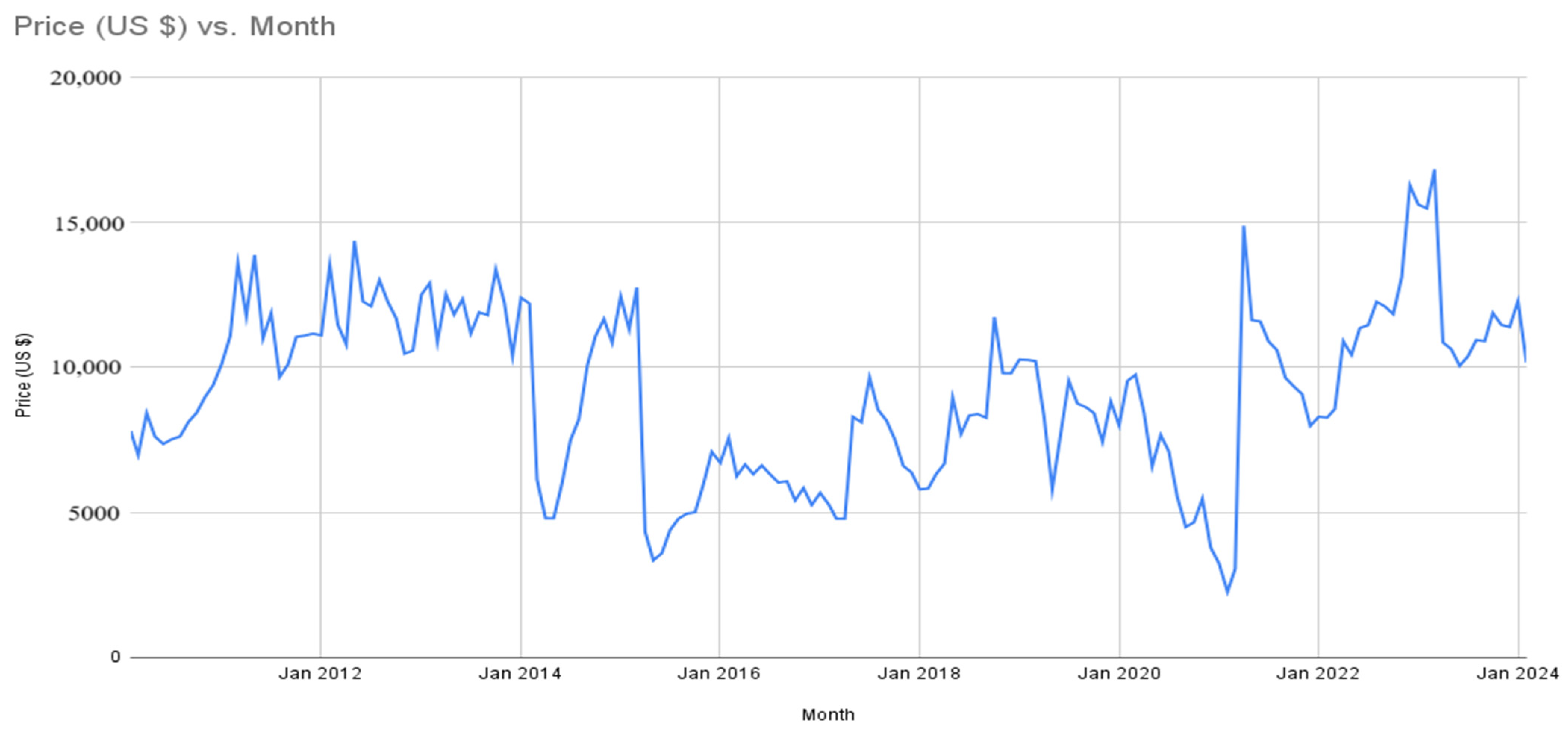
3.1. Data Description
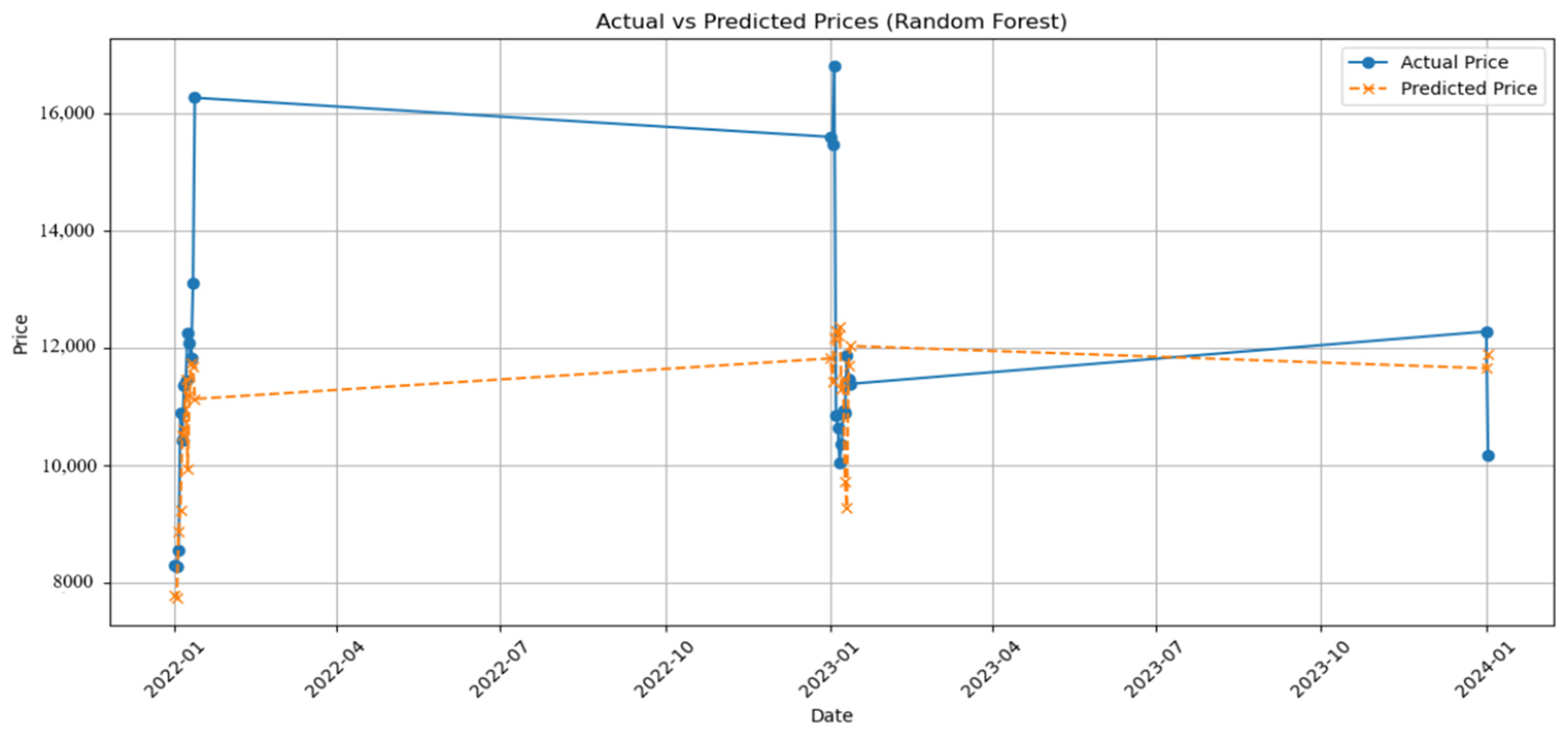
3.2. Random Forest
3.3. GRU
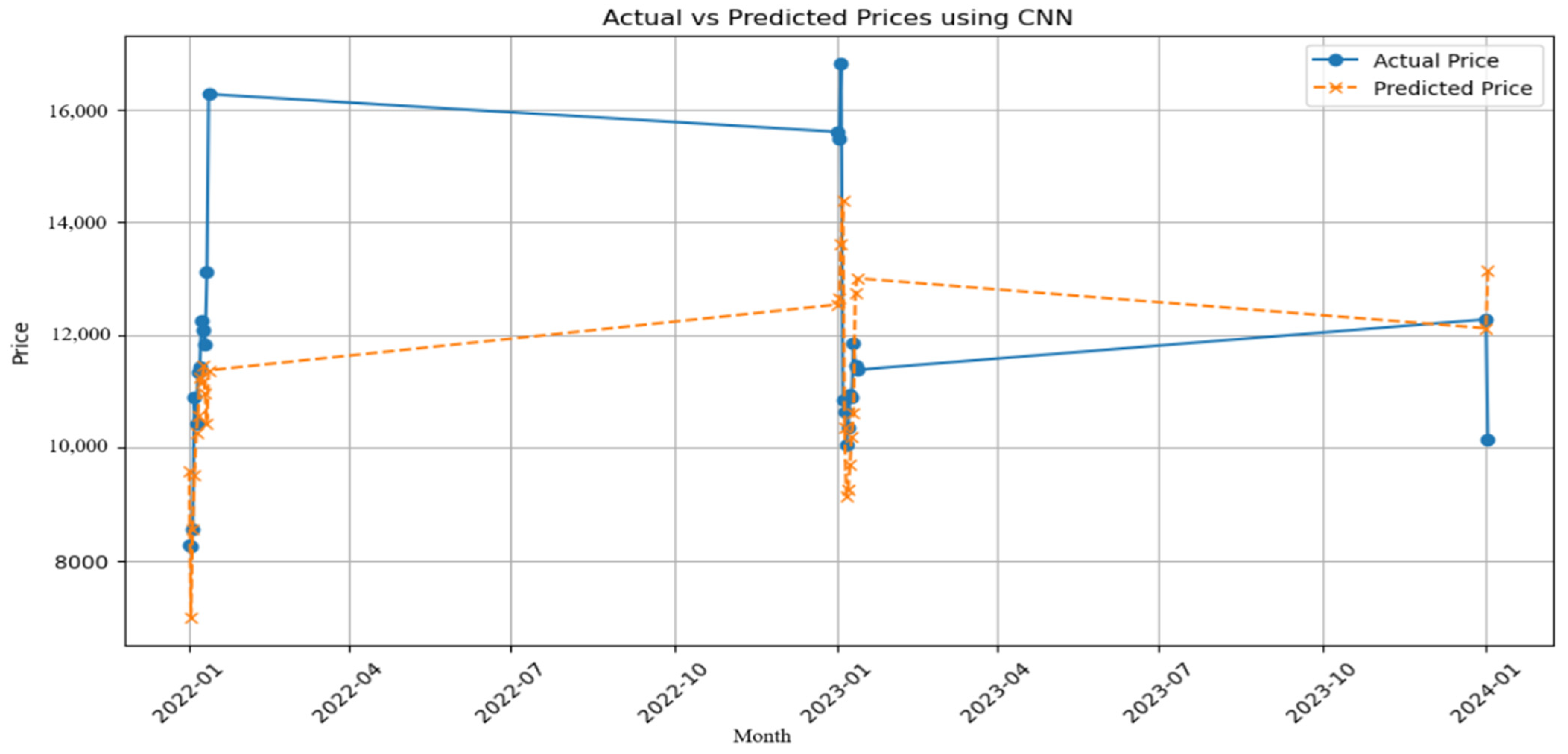
3.4. CNN
3.5. XGBoost
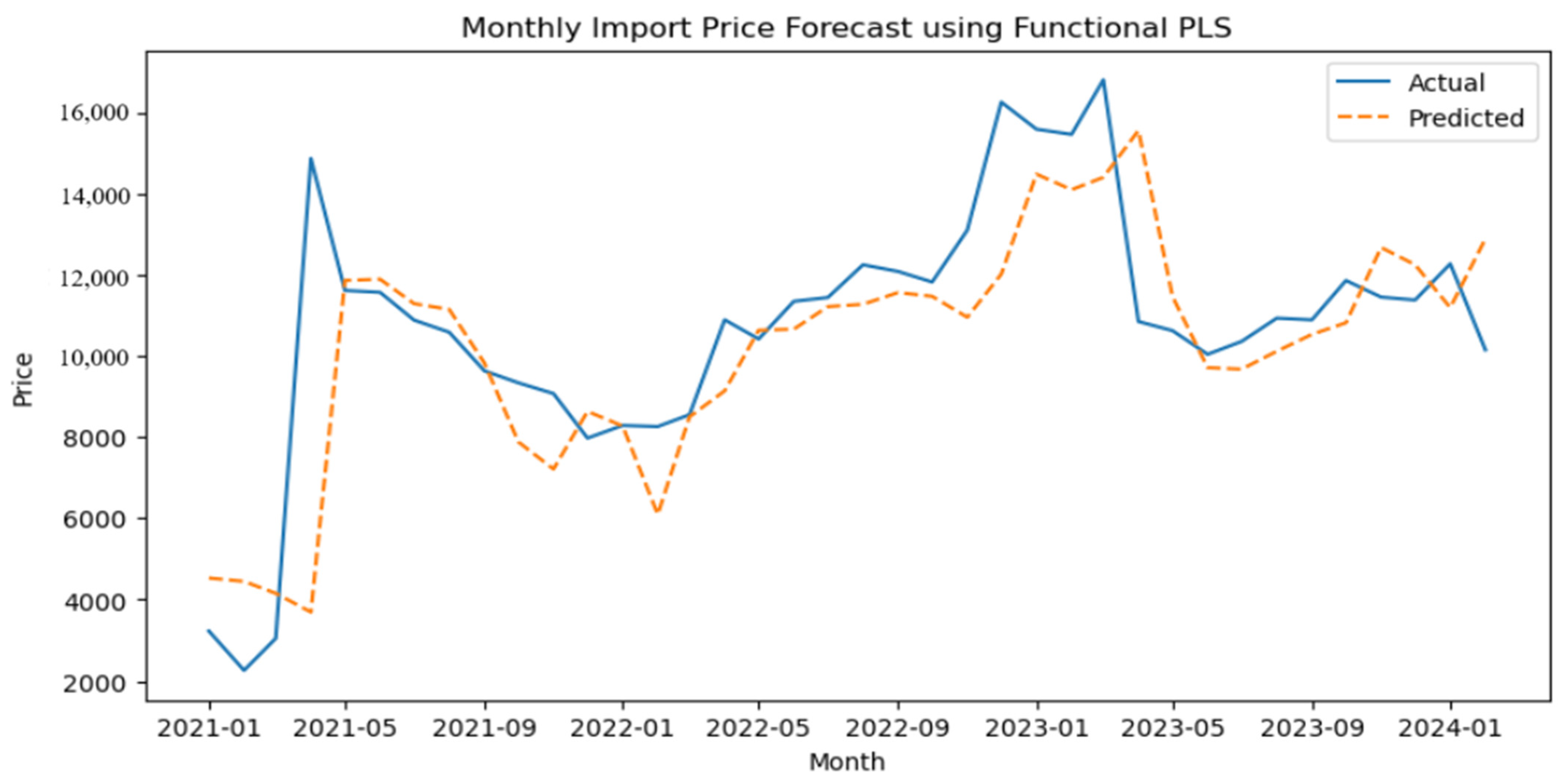
3.6. FPLS
3.7. Proposed Hybrid Model RF-GRU-CNN-XGBoost-FPLS-Stacking
3.8. Matrix Evaluation and Comparative Analysis
4. Conclusions
Author Contributions
Funding
Institutional Review Board Statement
Informed Consent Statement
Data Availability Statement
Conflicts of Interest
References
- Abdollahi, H. (2020). A novel hybrid model for forecasting crude oil price based on time series decomposition. Applied Energy, 267, 115035. [Google Scholar] [CrossRef]
- Alvarez-Ramirez, J., Cisneros, M., Ibarra-Valdez, C., & Soriano, A. (2002). Multifractal Hurst analysis of crude oil prices. Physica A: Statistical Mechanics and Its Applications, 313(3–4), 651–670. [Google Scholar] [CrossRef]
- Andrikopoulos, A., Merika, A., & Stoupos, N. (2025). The effect of oil prices on the US shipping stock prices: The mediating role of freight rates and economic indicators. Journal of Commodity Markets, 38, 100474. [Google Scholar] [CrossRef]
- Banik, R., & Biswas, A. (2024). Enhanced renewable power and load forecasting using RF-XGBoost stacked ensemble. Electrical Engineering, 106(4), 4947–4967. [Google Scholar] [CrossRef]
- Chai, J., Lu, Q., Hu, Y., Wang, S., Lai, K. K., & Liu, H. (2018). Analysis and bayes statistical probability inference of crude oil price change point. Technological Forecasting and Social Change, 126, 271–283. [Google Scholar] [CrossRef]
- Chen, J., Zhang, C., Li, X., He, R., Wang, Z., Nazir, M. S., & Peng, T. (2025). An integrative approach to enhance load forecasting accuracy in power systems based on multivariate feature selection and selective stacking ensemble modeling. Energy, 326, 136337. [Google Scholar] [CrossRef]
- Cheng, Z., Li, M., Sun, Y., Hong, Y., & Wang, S. (2024). Climate change and crude oil prices: An interval forecast model with interval-valued textual data. Energy Economics, 134, 107612. [Google Scholar] [CrossRef]
- Cui, J., Kuang, W., Geng, K., Bi, A., Bi, F., Zheng, X., & Lin, C. (2024). Advanced short-term load forecasting with XGBoost-RF feature selection and CNN-GRU. Processes, 12(11), 2466. [Google Scholar] [CrossRef]
- Delaigle, A., & Hall, P. (2012). Methodology and theory for partial least squares applied to functional data. Annals of Statistics, 40(1), 322–352. [Google Scholar] [CrossRef]
- Deng, S., Xiang, Y., Nan, B., Tian, H., & Sun, Z. (2020). A hybrid model of dynamic time wrapping and hidden Markov model for forecasting and trading in crude oil market. Soft Computing, 24, 6655–6672. [Google Scholar] [CrossRef]
- Ding, Y. (2018). A novel decompose-ensemble methodology with AIC-ANN approach for crude oil forecasting. Energy, 154, 328–336. [Google Scholar] [CrossRef]
- Ferraty, F. (2006). Nonparametric functional data analysis. Springer. [Google Scholar]
- Fozap, F. M. P. (2025). Hybrid machine learning models for long-term stock market forecasting: Integrating technical indicators. Journal of Risk and Financial Management, 18(4), 201. [Google Scholar] [CrossRef]
- Harikrishnan, G. R., & Sreedharan, S. (2025). Advanced short-term load forecasting for residential demand response: An XGBoost-ANN ensemble approach. Electric Power Systems Research, 242, 111476. [Google Scholar]
- He, K., Yu, L., & Lai, K. K. (2012). Crude oil price analysis and forecasting using wavelet decomposed ensemble model. Energy, 46(1), 564–574. [Google Scholar] [CrossRef]
- He, Y., Yan, Y., & Xu, Q. (2019). Wind and solar power probability density prediction via fuzzy information granulation and support vector quantile regression. International Journal of Electrical Power & Energy Systems, 113, 515–527. [Google Scholar]
- Huang, B., Sun, Y., & Wang, S. (2021). A new two-stage approach with boosting and model averaging for interval-valued crude oil prices forecasting in uncertainty environments. Frontiers in Energy Research, 9, 707937. [Google Scholar] [CrossRef]
- Jiang, Z., Dong, X., & Yoon, S. M. (2025). Impact of oil prices on key energy mineral prices: Fresh evidence from quantile and wavelet approaches. Energy Economics, 145, 108461. [Google Scholar] [CrossRef]
- Khan, M., Karim, S., Naz, F., & Lucey, B. M. (2025). How do exchange rate and oil price volatility shape pakistan’s stock market? Research in International Business and Finance, 2025, 102796. [Google Scholar] [CrossRef]
- Kim, M. S., Lee, B. S., Lee, H. S., Lee, S. H., Lee, J., & Kim, W. (2020). Robust estimation of outage costs in South Korea using a machine learning technique: Bayesian tobit quantile regression. Applied Energy, 278, 115702. [Google Scholar] [CrossRef]
- Kumari, K., Sharma, H. K., Chandra, S., & Kar, S. (2022). Forecasting foreign tourist arrivals in India using a single time series approach based on rough set theory. International Journal of Computing Science and Mathematics, 16(4), 340–354. [Google Scholar] [CrossRef]
- Li, J., Hong, Z., Zhang, C., Wu, J., & Yu, C. (2024). A novel hybrid model for crude oil price forecasting based on MEEMD and Mix-KELM. Expert Systems with Applications, 246, 123104. [Google Scholar] [CrossRef]
- Li, R., Hu, Y., Heng, J., & Chen, X. (2021). A novel multiscale forecasting model for crude oil price time series. Technological Forecasting and Social Change, 173, 121181. [Google Scholar] [CrossRef]
- Liang, Q., Lin, Q., Guo, M., Lu, Q., & Zhang, D. (2025). Forecasting crude oil prices: A gated recurrent unit-based nonlinear granger causality model. International Review of Financial Analysis, 102, 104124. [Google Scholar] [CrossRef]
- Liu, L., Zhou, S., Jie, Q., Du, P., Xu, Y., & Wang, J. (2024). A robust time-varying weight combined model for crude oil price forecasting. Energy, 299, 131352. [Google Scholar] [CrossRef]
- Ma, Y., Li, S., & Zhou, M. (2024). Forecasting crude oil prices: Does global financial uncertainty matter? International Review of Economics & Finance, 96, 103723. [Google Scholar]
- Manickavasagam, J., Visalakshmi, S., & Apergis, N. (2020). A novel hybrid approach to forecast crude oil futures using intraday data. Technological Forecasting and Social Change, 158, 120126. [Google Scholar] [CrossRef]
- Movagharnejad, K., Mehdizadeh, B., Banihashemi, M., & Kordkheili, M. S. (2011). Forecasting the differences between various commercial oil prices in the Persian Gulf region by neural network. Energy, 36(7), 3979–3984. [Google Scholar] [CrossRef]
- Oglend, A., & Kleppe, T. S. (2025). Storage scarcity and oil price uncertainty. Energy Economics, 144, 108393. [Google Scholar] [CrossRef]
- Petroleum planning and analysis cell of the government of India. (n.d.). Available online: https://ppac.gov.in/prices/international-prices-of-crude-oil (accessed on 26 December 2024).
- Preda, C., & Saporta, G. (2005). Clusterwise PLS regression on a stochastic process. Computational Statistics & Data Analysis, 49(1), 99–108. [Google Scholar]
- Qian, Q., Li, M., & Xu, J. (2022). Dynamic prediction of multivariate functional data based on functional kernel partial least squares. Journal of Process Control, 116, 273–285. [Google Scholar] [CrossRef]
- Ramsay, J. O., & Silverman, B. W. (2005). Principal components analysis for functional data. Functional Data Analysis, 2005, 147–172. [Google Scholar]
- Rao, A., Sharma, G. D., Tiwari, A. K., Hossain, M. R., & Dev, D. (2025). Crude oil price forecasting: Leveraging machine learning for global economic stability. Technological Forecasting and Social Change, 216, 124133. [Google Scholar] [CrossRef]
- Satija, A., & Caers, J. (2015). Direct forecasting of subsurface flow response from non-linear dynamic data by linear least-squares in canonical functional principal component space. Advances in Water Resources, 77, 69–81. [Google Scholar] [CrossRef]
- Sharma, H. K., & Kumari, K. (2025). Tourist arrivals demand forecasting using rough set-based time series models. Decision Making Advances, 3(1), 216–227. [Google Scholar] [CrossRef]
- Sharma, H. K., Kumari, K., & Kar, S. (2018). Air passengers forecasting for Australian airline based on hybrid rough set approach. Journal of Applied Mathematics, Statistics and Informatics, 14(1), 5–18. [Google Scholar] [CrossRef]
- Shen, L., Bao, Y., Hasan, N., Huang, Y., Zhou, X., & Deng, C. (2024). Intelligent crude oil price probability forecasting: Deep learning models and industry applications. Computers in Industry, 163, 104150. [Google Scholar] [CrossRef]
- Sun, J., Zhao, P., & Sun, S. (2022). A new secondary decomposition-reconstruction-ensemble approach for crude oil price forecasting. Resources Policy, 77, 102762. [Google Scholar] [CrossRef]
- Sun, J., Zhao, X., & Xu, C. (2021). Crude oil market autocorrelation: Evidence from multiscale quantile regression analysis. Energy Economics, 98, 105239. [Google Scholar] [CrossRef]
- Tang, Q., Li, H., Feng, S., Guo, S., Li, Y., Wang, X., & Zhang, Y. (2025). Predicting the changes in international crude oil trade relationships via a gravity heuristic algorithm. Energy, 322, 135567. [Google Scholar] [CrossRef]
- Ullah, S., Chen, X., Han, H., Wu, J., Liu, R., Ding, W., Liu, M., Li, Q., Qi, H., Huang, Y., & Yu, P. L. (2025). A novel hybrid ensemble approach for wind speed forecasting with dual-stage decomposition strategy using optimized GRU and Transformer models. Energy, 2025, 136739. [Google Scholar] [CrossRef]
- Wang, D., Lu, Z., Liu, Z., Xue, S., Guo, M., & Hou, Y. (2025). A functional mixture prediction model for dynamically forecasting cumulative intraday returns of crude oil futures. International Journal of Forecasting. in press. [Google Scholar]
- Wang, J., Zhou, H., Hong, T., Li, X., & Wang, S. (2020). A multi-granularity heterogeneous combination approach to crude oil price forecasting. Energy Economics, 91, 104790. [Google Scholar] [CrossRef]
- Wei, H., & Liu, Y. (2025). Commodity import price rising and production stability of Chinese firms. Structural Change and Economic Dynamics, 73, 434–448. [Google Scholar] [CrossRef]
- Xu, Y., Liu, T., Fang, Q., Du, P., & Wang, J. (2025). Crude oil price forecasting with multivariate selection, machine learning, and a nonlinear combination strategy. Engineering Applications of Artificial Intelligence, 139, 109510. [Google Scholar] [CrossRef]
- Yang, C. W., Hwang, M. J., & Huang, B. N. (2002). An analysis of factors affecting price volatility of the US oil market. Energy Economics, 24(2), 107–119. [Google Scholar] [CrossRef]
- Yang, Y., Guo, J. E., Sun, S., & Li, Y. (2021). Forecasting crude oil price with a new hybrid approach and multi-source data. Engineering Applications of Artificial Intelligence, 101, 104217. [Google Scholar] [CrossRef]
- Zhang, C., & Zhou, X. (2024). Forecasting value-at-risk of crude oil futures using a hybrid ARIMA-SVR-POT model. Heliyon, 10(1), e23358. [Google Scholar] [CrossRef]
- Zhang, J., & Liu, Z. (2024). Interval prediction of crude oil spot price volatility: An improved hybrid model integrating decomposition strategy, IESN and ARIMA. Expert Systems with Applications, 252, 124195. [Google Scholar] [CrossRef]
- Zhang, W., Wu, J., Wang, S., & Zhang, Y. (2025). Examining dynamics: Unraveling the impact of oil price fluctuations on forecasting agricultural futures prices. International Review of Financial Analysis, 97, 103770. [Google Scholar] [CrossRef]
- Zhao, S., Wang, Y., Deng, J., Li, Z., Deng, G., Chen, Z., & Li, Y. (2025). An adaptive multi-factor integrated forecasting model based on periodic reconstruction and random forest for carbon price. Applied Soft Computing, 177, 113274. [Google Scholar] [CrossRef]


| Model | Pros | Cons |
|---|---|---|
| GRU | Captures temporal dependencies well | Lags at sharp changes; may overfit with small data |
| CNN | Detects local patterns; captures spatial temporal patterns | Prone to overshooting; needs lots of training data |
| XGBoost | Non-linear and stable | Misses temporal nuance; may lag at turning points |
| Random Forest | Good at fitting and non-linear trends | Sensitive to lag selection; unstable transitions; overfits and noisy |
| FPLS | Captures trend; robust to noise | Misses volatility; Underestimates spikes |
| RF-GRU-CNN- XGBoost-FPLS-Stacking | Combines strengths; generalizes well | More complex; requires tuning and base diversity |
| Month | Actual Price | Random Forest | CNN | XGBoost | GRU | FPLS | RF-GRU-CNN- XGBoost- FPLS-Stacking |
|---|---|---|---|---|---|---|---|
| Jan 2021 | 10,887 | 11,693 | 11,390 | 7754.9 | 11,689 | 4531 | 10,730 |
| Feb 2021 | 10,589 | 12,093 | 10,860 | 8377.1 | 10,927 | 4448.2 | 10,795 |
| Mar 2021 | 9637 | 11,281 | 12,477 | 8377.1 | 10,232 | 4154.5 | 10,364 |
| Apr 2021 | 9340 | 9514.9 | 11,743 | 8377.1 | 9421.4 | 3694.3 | 9385 |
| May 2021 | 9075 | 9148.2 | 9743.5 | 8922.2 | 8976.3 | 11,866 | 9072.3 |
| Jun 2021 | 7976 | 8713.9 | 9491.5 | 8637.7 | 8921.2 | 11,897 | 8617.3 |
| Jul 2021 | 8289 | 8543.6 | 9193.2 | 8637.7 | 8501.3 | 11,293 | 8606.4 |
| Aug 2021 | 8262 | 8327.7 | 9208.2 | 8922.2 | 8517 | 11,153 | 8774.4 |
| Sep 2021 | 8555 | 9319.6 | 10,036 | 7754.9 | 9117.4 | 9831.7 | 8938 |
| Oct 2021 | 10,895 | 8906.2 | 10,514 | 7754.9 | 9838 | 7883 | 10,675 |
| Nov 2021 | 10,421 | 11,371 | 12,461 | 7754.9 | 11,169 | 7212.5 | 10,581 |
| Dec 2021 | 11,351 | 11,273 | 13,017 | 7754.9 | 11,727 | 8635.5 | 11,075 |
| Jan 2022 | 11,445 | 11,694 | 13,926 | 7754.9 | 12,507 | 8275.3 | 11,476 |
| Feb 2022 | 12,253 | 11,050 | 14,413 | 8377.1 | 12,836 | 6092.8 | 12,033 |
| Mar 2022 | 12,087 | 11,787 | 15,384 | 8377.1 | 13,106 | 8502.5 | 12,236 |
| Apr 2022 | 11,827 | 11,950 | 15,050 | 8377.1 | 12,957 | 9142.5 | 11,881 |
| May 2022 | 13,107 | 11,917 | 13,561 | 8922.2 | 12,440 | 10,637 | 13,370 |
| Jun 2022 | 16,265 | 11,776 | 13,623 | 8637.7 | 12,488 | 10,664 | 14,725 |
| Jul 2022 | 15,597 | 12,492 | 13,614 | 8637.7 | 13,402 | 11,220 | 14,890 |
| Aug 2022 | 15,469 | 13,800 | 12,483 | 8922.2 | 13,089 | 11,278 | 14,549 |
| Sep 2022 | 16,815 | 14,729 | 12,033 | 7754.9 | 12,389 | 11,567 | 14,704 |
| Oct 2022 | 10,852 | 15,677 | 12,193 | 7754.9 | 12,111 | 11,474 | 12,245 |
| Nov 2022 | 10,628 | 12,395 | 10,923 | 7754.9 | 9497 | 10,958 | 10,981 |
| Dec 2022 | 10,044 | 11,065 | 10,511 | 7754.9 | 8253.5 | 12,022 | 10,309 |
| Jan 2023 | 10,362 | 10,006 | 9755.1 | 7754.9 | 7727.3 | 14,489 | 10,505 |
| Feb 2023 | 10,936 | 10,156 | 9708.5 | 8377.1 | 7904.5 | 14,105 | 10,929 |
| Mar 2023 | 10,894 | 11,303 | 9366.7 | 8377.1 | 8616.8 | 14,409 | 11,068 |
| Apr 2023 | 11,864 | 11,160 | 9128.8 | 8377.1 | 9380 | 15,566 | 11,458 |
| May 2023 | 11,455 | 11,683 | 10,900 | 8922.2 | 10,517 | 11,469 | 11,242 |
| Jun 2023 | 11,383 | 12,290 | 11,813 | 8637.7 | 10,988 | 9714.9 | 11,322 |
| Jul 2023 | 12,276 | 11,990 | 12,442 | 8637.7 | 11,058 | 9677.1 | 11,543 |
| Aug 2023 | 10,154 | 11,936 | 12,836 | 8922.2 | 11,362 | 10,119 | 10,392 |
| Sep 2023 | 10,894 | 9710 | 9914 | 11,173 | 10,683 | 10,536 | 10,961 |
| Oct 2023 | 11,864 | 9277 | 10,621 | 7806 | 10,642 | 10,822 | 11,241 |
| Nov 2023 | 11,455 | 11,692 | 12,601 | 11,203 | 11,105 | 12,680 | 11,498 |
| Dec 2023 | 11,383 | 12,030 | 13,184 | 11,865 | 10,993 | 12,253 | 11,486 |
| Jan 2024 | 12,276 | 11,649 | 12,519 | 11,388 | 10,935 | 11,196 | 11,617 |
| Feb 2024 | 10,154 | 11,894 | 13,112 | 11,350 | 11,374 | 12,892 | 10,628 |
| Errors | Random Forest | XGBoost | CNN | GRU | FPLS | RF-GRU-CNN- XGBoost- FPLS-Stacking |
|---|---|---|---|---|---|---|
| MAPE | 13.82% | 16.26% | 14.08% | 10.86% | 15.39% | 3.45% |
| MAE | 1380.5 | 3433.1 | 1614.4 | 1302.4 | 1432.2 | 410.48 |
| MASE | 1394 | 40.882 | 1.8287 | 1.4752 | 0.4663 | |
| RMSE | 1385.1 | 1971.6 | 1680.4 | 2389.1 | 607.98 | |
| RMSSE | 1379 | 4033.5 | 1.3456 | 1.147 | 1.274 | 0.4313 |
| MSE | 1386.7 | 4033.5 | 1.3074 |
Disclaimer/Publisher’s Note: The statements, opinions and data contained in all publications are solely those of the individual author(s) and contributor(s) and not of MDPI and/or the editor(s). MDPI and/or the editor(s) disclaim responsibility for any injury to people or property resulting from any ideas, methods, instructions or products referred to in the content. |
© 2025 by the authors. Licensee MDPI, Basel, Switzerland. This article is an open access article distributed under the terms and conditions of the Creative Commons Attribution (CC BY) license (https://creativecommons.org/licenses/by/4.0/).
Share and Cite
Choudhary, J.; Sharma, H.K.; Malik, P.; Majumder, S. Price Forecasting of Crude Oil Using Hybrid Machine Learning Models. J. Risk Financial Manag. 2025, 18, 346. https://doi.org/10.3390/jrfm18070346
Choudhary J, Sharma HK, Malik P, Majumder S. Price Forecasting of Crude Oil Using Hybrid Machine Learning Models. Journal of Risk and Financial Management. 2025; 18(7):346. https://doi.org/10.3390/jrfm18070346
Chicago/Turabian StyleChoudhary, Jyoti, Haresh Kumar Sharma, Pradeep Malik, and Saibal Majumder. 2025. "Price Forecasting of Crude Oil Using Hybrid Machine Learning Models" Journal of Risk and Financial Management 18, no. 7: 346. https://doi.org/10.3390/jrfm18070346
APA StyleChoudhary, J., Sharma, H. K., Malik, P., & Majumder, S. (2025). Price Forecasting of Crude Oil Using Hybrid Machine Learning Models. Journal of Risk and Financial Management, 18(7), 346. https://doi.org/10.3390/jrfm18070346