Forecasting Systemic Risk in the European Banking Industry: A Machine Learning Approach

Abstract

The aim of this article is to forecast the systemic risk contribution and exposure measured by the delta conditional value at risk (ΔCoVaR) and the marginal expected shortfall (MES), respectively. We first estimate the ΔCoVaR and MES for banks in 16 European countries for the 2002–2016 period. We then predict systemic risk measures using machine learning techniques, such as artificial neural network (ANN) and support vector machine (SVM), and we use AR-GARCH specification. Finally, we compare the methods’ forecasting values and the actual values. Our results show that two hidden layers of artificial neural networks perform efficiently in forecasting systemic risk.

1. Introduction

Financial institutions play a crucial role in the functioning of an economy. Banks, in particular, perform vital functions that are unique in their nature. This uniqueness stems from the fact that banks mainly accept deposits of short maturity and make loans of long maturity. This mismatch between the sources and uses of funds, combined with a number of other factors and characteristics of banking, exposes banks to a number of risks, which may in times of distress threaten the well being of the entire economy or large segments thereof.

In light of the multiple risks that banks face, and the potential negative externalities they could cause for the rest of the economy, they have been heavily supervised and regulated, especially in industrial countries. As controversial as the question of regulations is, “a central issue in this controversy is the extent to which, a negative event, occurring at a specific bank, that implies an increase in the probability of its failure, generates negative externalities for the banking system.” (Slovin et al., 1999, p. 198). This is what is loosely referred to as systemic banking risk.

Generally defined as the risk of a collapse in the entire banking system, which typically breaks due to the default of one, or more, typically interconnected banks, systemic risk gained great attention in policy, academic, and research circles following the failure of Lehman Brothers in 2008 and the contagion effect that accompanied it as the global financial crisis of 2007–2009 unfolded and spread out (Borri et al., 2012).

Accordingly, during the last decade or so, research has shifted toward the measurement and estimation of systemic risk (e.g., Roy, 2023; Kyoud et al., 2023; Acharya et al., 2017; Brownlees & Engle, 2012; Girardi & Tolga Ergün, 2013; Bisias et al., 2012). Yet, research on banking failure dates back to the late 1970s, following a couple of business failure prediction studies by Beaver (1966) and Altman (1968). To that extent, prediction methods evolved from the use of traditional financial ratios to the implementation of sophisticated linear, multivariate, and quadratic discriminant analysis techniques, as well as logistic regression functions (Liu et al., 2021).

However, rapid recent advancements in artificial intelligence and machine learning technologies have made it possible to potentially overcome the limitations of statistical techniques and develop more robust prediction models. Indeed, as Le and Viviani (2018) mention, machine learning techniques (MLTs) are increasingly being used, including mainly artificial neural networks (ANNs), support vector machines (SVMs), and k-nearest neighbor algorithms (KNNs).

Attempting to leverage rapidly evolving advancements in artificial intelligence and machine learning for a better understanding of systemic risk, and consequently to contribute to the development of more robust systemic risk forecasting models, by addressing an apparent gap in the empirical and practical research of systemic risk prediction, the objective of this study is threefold. First, we measure the systemic risk contribution and exposure of European banks using the ΔCoVaR and the MES, respectively, for the period from 2002 to 2016, which corresponds to a framework of ex ante, during, and ex post the global financial crisis of 2007–2009. Second, we forecast the systemic risk using artificial neural networks (ANNs) and support vector machines (SVMs), two of the most used machine learning methods, and we use generalized autoregressive conditional heteroscedasticity (GARCH), a volatility estimating tool. Finally, we compare the forecasted values with the measured values to determine the effectiveness of our machine learning approach. To the best of our knowledge, no other studies have specifically combined the use of these three algorithms and compared the results in forecasting systemic risk.

This paper is organized as follows. Section 2 presents the literature review, while Section 3 covers the methodology. In Section 4, we describe the sample and report the prediction elaboration. The results are then discussed and concluded in Section 5.

2. Literature Review

Definitions of systemic risk started to appear in the literature in the mid-1990s. Yet, elaboration of such definitions intensified after the outbreak of the global financial crisis of 2007–2009. Smaga (2014) states that “before the crisis, definitions put more emphasis on the contagion effect and the large scale of this phenomenon. However, after the outbreak of the crisis, in addition to the significant scale of the phenomenon, more attention has been paid to disturbances in financial system functions. This results in defaults and has a negative impact on the real economy, which in turn was rarely underlined before the crisis.” In their extensive review of the systemic risk literature, Galati and Moessner (2010) conclude that there is no single common definition of systemic risk. Bisias et al. (2012) and Osterloo and De Haan (2003) demonstrate that different definitions emphasize different aspects of systemic risks, such as imbalances, loss of confidence, feedback effects, and negative externalities.

A lack of consensus about the conceptualization and the definition of systemic risk poses challenges for its measurement and operationalization. Yet, there is one thing that is certain in the materialization of systemic risk, and it was evident during the global financial crisis. It is the interconnectedness between the contribution of a financial institution to systemic risk and its exposure to it. Consequently, contribution and exposure have been taken in the literature as measurement proxies for systemic risk.

One widely used cross-sectional measure of systemic risk is the conditional value at risk (CoVaR) developed by Adrian and Brunnermeier (2010, 2016). Unlike the value at risk (VaR) that measures the risk of a firm in isolation, the CoVaR measures the risk of a financial firm(s) conditional upon the financial distress of other institution(s) or of the overall distress of the entire system. Researchers also developed the delta CoVaR (ΔCoVaR), which measures the contribution of each institution to systemic risk. In addition to measuring firms’ systemic risk contribution, Acharya et al. (2017) measured the exposure of each bank to overall systemic risk using the marginal expected shortfall (MES). In this paper, we focus our attention on these two measures to capture the contribution and the exposure of each bank to systemic risk.

In addition to the measurement of systemic risk and contribution, we employ a machine learning approach to forecast systemic risk, namely, artificial neural networks (ANNs) and support vector machines (SVMs). Initially developed by McCulloch and Pitts (1943)1, ANNs are artificial intelligence quantitative models based on the human brain structure and functionality. The motivation behind ANNs was to create artificial systems able to do difficult and complicated computations analogous to those performed by the human brain, such as pattern recognition.2 ANNs are data processing techniques that are capable of detecting, learning, and predicting complex relations between quantities by repeatedly presenting examples of the relationship to the network.

In recent years, neural networks have been successfully used for modeling financial time series. Neural networks are data-driven3, non-parametric models, and they are specialized by their capability to learn complex systems with incomplete and corrupted data. In addition, they are flexible and have the ability to learn dynamic systems through a retraining process using new patterns of the data. These characteristics make the ANN more powerful in describing the financial time series rather than the traditional statistical models (Tay & Cao, 2001).

While systemic risk arises from the non-linear complex relationship between institutions, neural networks can model these complex links that traditional models miss. Moreover, neural networks can process multivariate time series and complex datasets with several inputs, making them suitable for systemic risk quantification. Additionally, systemic risk can arise from unseen correlations or contagion channels, which can be detected by neural networks with deep architectures.

Another machine learning method in the domain of artificial intelligence is support vector machines (SVMs) introduced by Vapnik (1995). SVMs are developed to resolve classification problems, but they have recently used as a regression tool.

The main idea of an SVM algorithm is to construct an optimal separating hyperplane with high classification accuracy. It builds a model that can assign new examples to one of two categories based on a set of training examples. In an SVM model, examples are represented as points in space in a way that points belonging to different categories are separated by a clear gap. This separation then maps the new examples into this space in their corresponding categories. When using an SVM to estimate the regression, three distinct characteristics are satisfied. First, the regression is estimated using a set of linear functions defined in a high dimensional space.4 Second, in SVMs, the regression estimation is established by minimizing the risk measure by the loss function. Third, the risk function used by SVMs consists of the empirical error and the regularization term derived from the structural risk minimization principle (Tay & Cao, 2001).

Systemic risk can be viewed as a classification approach, e.g., is an institution/system in a high-risk or low-risk state? SVMs are able to classify them by identifying vulnerable institutions, predicting cascading failures, or classifying risk levels across the financial system by creating the optimal separation vector.

The last prediction method used in this study to model time series is the generalized autoregressive conditional heteroskedasticity (GARCH) process developed by Engle (1982) as an econometric tool to estimate volatility in financial markets. The main idea behind the GARCH specification is that observations, especially in finance, do not always conform to a linear pattern. Instead, they tend to cluster in irregular patterns and have high error variation. GARCH models were introduced to deal with volatility variation among observations.

To our knowledge, there is no article focused on forecasting systemic risk and comparing the effectiveness of these three algorithms we reviewed. In this study, we adopt this point of view by predicting the systemic risk contribution measured by the ΔCoVaR and the systemic risk exposure measured by the MES for the European banking sector composed of 134 banks in 16 European countries from 2002 to 2016. We also focus on comparing the performance of the three models, namely, the ANN, SVM, and AR-GARCH, in predicting systemic risk in the European banking sector.

Our results show that neural networks outperform the support vector machine regression and the GARCH specification in predicting systemic risk for our sample, highlighting the fact that the systemic risk is complex and deep in structure. Moreover, we show that the two hidden layer neural network was more adequate than one hidden layer neural network. Our results contribute to the existing debate about predicting systemic risk by presenting an efficient tool to prevent, perhaps, or at least lessen, some systemic risk consequences.

3. Methodology

In this section, we present the details of measuring and forecasting systemic risk. Our methodology involves three steps. In the first step, we estimate the systemic risk contribution by calculating the value at risk (VaR), the conditional value at risk (CoVaR), and the delta CoVaR (ΔCoVaR) via quantile regressions using a set of financial, market, and state factors as explanatory variables. We also estimate the systemic risk exposure using the marginal expected shortfall (MES). In the second step, we perform systemic risk forecasting. We use the results obtained in the first step (i.e., ΔCoVaR and MES) to implement two artificial neural networks, a support vector machine regression, and an AR-GARCH(1,1) specification model. Finally, in the last step, we estimate the accuracy of the forecasting methods by comparing the predicted values with the actual values. Details of each of the above-mentioned steps are presented below.

3.1. Step 1: Measuring Systemic Risk

In this paper, we aim to forecast the systemic risk contribution and exposure of the European banking sector. To measure the systemic risk contribution of banks, we use the delta conditional value at risk (ΔCoVaR) proposed by Adrian and Brunnermeier (2016). We use the marginal expected shortfall (MES) proposed by Acharya et al. (2017) to estimate the exposure of each bank to the systemic risk.

We first estimate the system’s conditional value at risk (CoVaR), which is the value at risk (VaR) of the system if a particular institution is under financial distress.5 Following Adrian and Brunnermeier (2016), we collect the accounting variables and market data used in the following quantile regression equations:

$$\left\{\begin{array}{c}{\mathrm{R}}_{\mathrm{t}}^{\mathrm{i}}={\mathsf{\alpha }}_{\mathrm{q}}^{\mathrm{i}}+{\mathsf{\gamma }}_{\mathrm{q}}^{\mathrm{i}}* {\mathrm{M}}_{\mathrm{t}-1}+{\mathsf{\epsilon }}_{\mathrm{q},\mathrm{t}}^{\mathrm{i}}\\ {\mathrm{R}}_{\mathrm{t}}^{\mathrm{s}|\mathrm{i}}={\mathsf{\alpha }}_{\mathrm{q}}^{\mathrm{s}|\mathrm{i}}+{\mathsf{\beta }}_{\mathrm{q}}^{\mathrm{s}|\mathrm{i}}* {\mathrm{R}}_{\mathrm{t}}^{\mathrm{i}}+{\mathsf{\gamma }}_{\mathrm{q}}^{\mathrm{s}|\mathrm{i}}* {\mathrm{M}}_{\mathrm{t}-1}+{\mathsf{\epsilon }}_{\mathrm{q},\mathrm{t}}^{\mathrm{s}|\mathrm{i}}\end{array}\right.$$

(1)

where ${\mathrm{R}}_{\mathrm{t}}^{\mathrm{i}}$ is the return6 of the bank i at time t defined as $\mathrm{l}\mathrm{n}\left({\displaystyle \frac{{\mathrm{P}}_{\mathrm{t}}^{\mathrm{i}}}{{\mathrm{P}}_{\mathrm{t}-1}^{\mathrm{i}}}}\right)$, where ${\mathrm{P}}_{\mathrm{t}}^{\mathrm{i}}$ is the price of the stock i at time $t. {\mathrm{M}}_{\mathrm{t}-1}$ is a vector of lagged state variables that includes the volatility index (V2X), which captures the implied volatility in the stock market, liquidity spread, which is the difference between the three-month repo rate and the three-month bill rate, the change in the three-month bill rate, the change in the slope of the yield curve, which is the difference between the German ten-year government bond yield and the German three-month Bubill rate, the change in credit spread, measured by the spread between ten-year Moody’s seasoned BAA-rated corporate bonds, and finally, the German ten-year government bond and the S&P 500 return index as a proxy for market equity returns (Anginer et al., 2014; Adrian & Brunnermeier, 2016). ${\mathrm{R}}_{\mathrm{t}}^{\mathrm{s}|\mathrm{i}}$ is the return of the system s conditional on the return of the bank i at time t, and ${\mathsf{\epsilon }}_{\mathrm{t}}^{\mathrm{i}}$ and ${\mathsf{\epsilon }}_{\mathrm{q},\mathrm{t}}^{\mathrm{s}|\mathrm{i}}$ are the error terms.

We then use the predicted values from the regression in Equation (1) to obtain the following:

$$\left\{\begin{array}{c}{\mathrm{V}\mathrm{a}\mathrm{R}}_{\mathrm{q},\mathrm{t}}^{\mathrm{i}}={\widehat{\mathsf{\alpha }}}_{\mathrm{q}}^{\mathrm{i}}+{\widehat{\mathsf{\gamma }}}_{\mathrm{q}}^{\mathrm{s}|\mathrm{i}}* {\mathrm{M}}_{\mathrm{t}-1}\\ {\mathrm{C}\mathrm{o}\mathrm{V}\mathrm{a}\mathrm{R}}_{\mathrm{q},\mathrm{t}}^{\mathrm{s}|\mathrm{i}}={\widehat{\mathsf{\alpha }}}_{\mathrm{q}}^{\mathrm{s}|\mathrm{i}}+{\widehat{\mathsf{\beta }}}_{\mathrm{q}}^{\mathrm{s}|\mathrm{i}}* {\mathrm{V}\mathrm{a}\mathrm{R}}_{\mathrm{q},\mathrm{t}}^{\mathrm{i}}+{\widehat{\mathsf{\gamma }}}_{\mathrm{q}}^{\mathrm{s}|\mathrm{i}}* {\mathrm{M}}_{\mathrm{t}-1}\end{array}\right.$$

(2)

where ${\mathrm{V}\mathrm{a}\mathrm{R}}_{\mathrm{q},\mathrm{t}}^{\mathrm{i}}$ is the VaR7 of the institution i at time t and $\mathrm{C}\mathrm{o}{\mathrm{V}\mathrm{a}\mathrm{R}}_{\mathrm{q},\mathrm{t}}^{\mathrm{s}|\mathrm{i}}$ is the VaR of the system s conditional on the distress situation of the institution i (i.e., when it is at its ${\mathrm{V}\mathrm{a}\mathrm{R}}_{\mathrm{q},\mathrm{t}}^{\mathrm{i}}$) at time t.

Finally, the contribution of each bank to the system’s risk is obtained using the ΔCoVaR as follows:

$${∆\mathrm{C}\mathrm{o}\mathrm{V}\mathrm{a}\mathrm{R}}_{\mathrm{q},\mathrm{t}}^{\mathrm{s}|\mathrm{i}}={\mathrm{C}\mathrm{o}\mathrm{V}\mathrm{a}\mathrm{R}}_{\mathrm{q},\mathrm{t}}^{\mathrm{s}|\mathrm{i}}-{\mathrm{C}\mathrm{o}\mathrm{V}\mathrm{a}\mathrm{R}}_{0.5,\mathrm{t}}^{\mathrm{s}|\mathrm{i}}$$

(3)

Equation (3) points out that the contribution of each bank to the systemic risk is the difference between the system’s VaR when the bank i is at its qth percentile and the VaR of the system when the bank i is at its median (i.e., normal situation). We compute ΔCoVaR at q = 1% for each bank of the sample from 2002 to 2016.

Next, following Acharya et al. (2017), we measure a bank’s systemic risk exposure by its marginal expected shortfall (MES), which is the mean return of the bank during times of a market crash. Formally, the MES of bank i at time t is given by the following formula:

$${\mathrm{M}\mathrm{E}\mathrm{S}}_{\mathrm{i},\mathrm{t}}\left(\mathrm{q}\right)=\mathrm{E}\left[{\mathrm{R}}_{\mathrm{i},\mathrm{t}}\left|{\mathrm{R}}_{\mathrm{m},\mathrm{t}}<{\mathrm{V}\mathrm{a}\mathrm{R}}_{\mathrm{m},\mathrm{t}}\left(\mathrm{q}\right)\right.\right]$$

(4)

where ${\mathrm{R}}_{\mathrm{i},\mathrm{t}}$ denotes the weekly stock return of bank i at time t and ${\mathrm{R}}_{\mathrm{m},\mathrm{t}}$ is the return of the market system8 at time t. Since the return indices for all countries are not available, we construct the market-weighted return and exclude the bank for which the MES is calculated from the banking sector. ${VaR}_{m,t}\left(q\right)$ denotes the q-value-at-risk of the market m at time t, which is the maximum value such that the probability of loss that exceeds this value equals to q. In other words, in Equation (4), we take the q = 1% worst days for the market returns in each given year, and we then compute the average return on each bank for these days.

3.2. Step 2: Forecasting Systemic Risk

After estimating systemic risk in the first step, in this paragraph, we present the methods used to forecast the systemic risk contribution and exposure of each bank of the sample, which are the artificial neural network (ANN), the support vector machine (SVM), and regressions—two machine learning methods and autoregressive plus generalized autoregressive conditional heteroscedasticity (AR-GARCH) specifications. The regressions are volatility clustering tools. Further details about methods implementation are provided thereafter in Section 3.2.

3.2.1. Artificial Neural Network (ANN)

Neural networks are universal function approximates that can map any non-linear function without a priori assumptions about the properties of the data (Haykin, 1994).9 They learn from examples using a training set; in other words, the network is capable of connecting inputs with outputs through estimated parameters, thus creating some sort of generalization beyond the training data. Networks are distinguished by their architectures, level of complexity10, number of layers11, presence of feedback loops12, and the activation or transfer function.13

Formally speaking, a neural network is a connection of elementary objects. Inputs $\left(x_1,\dots ,x_n\right)$, and weights14 $\left(w_1,\dots ,w_n\right)$, where weights $w_i$ $\in$ [0, 1] are associated with each input. The activation function $f$ is used to limit the output of the neuron. The combiner15 and the final output16 are obtained after the application of such an activation function. The final output $y$ is obtained by the following formula:

$$y=f(b+\sum _{i=1}^n{w}_i{x}_i)$$

(5)

where $x_i$ is systemic risk values (i.e., ΔCoVaR and MES) calculated in the first step; $f$ is the activation function; $n$ is the number of observations in the training dataset; $w_i$ is the weights associated with the nodes; and $b$ is an external bias. We split our data into three parts: 70% for training, 15% for validation, and 15% for testing. Another split percentage is 80% for training and 20% for testing and validation (Majumder et al., 2024). The first subset, the training data, consists of the estimated values of the ΔCoVaR and MES used to train the network and to fit the parameters of the classifier. The second subset, the validation data, is used to tune the parameters of the classifier and to find the optimal number of hidden units or determine a stopping point for the back-propagation algorithm. The third subset, the test dataset, is used to assess the performance of a fully trained classifier and to estimate the error rate to calculate the level of accuracy. Choosing the number of hidden layers in a multilayer network is not an easy subject. While Lee et al. (2005) and Zhang et al. (1999) argue that constructing a network with one hidden layer may resolve most of the classification problems, Vasu and Ravi (2011) show that networks with two hidden layers ensure the complexity of network architectures.

In our study, we implement a network composed of both one and two hidden layers to ensure the sufficiency of the complexity of the banking sector and examine which one performs better. Further details about the method are provided in Appendix A.

3.2.2. Support Vector Machine Regression (SVM)

The basic idea of the support vector machine is to construct a separating hyper-plane with a high level of accuracy.

Let $x_i=(x^1,\dots , x^p)$ be a set of inputs and $y_i$ be the corresponding target values, where $i=1,\dots ,n$ and $n$ is the size of the training set. Our goal is to find a function $f\left(x\right)$ that estimates the relation between the inputs and the target value.

The input vector in our study is systemic risk values: the contribution and the exposure of each bank to the systemic risk for the entire period. Regression uses a loss function $L(y$, $f\left(x\right)$) that shows how the estimated function $f$ deviates from the true values $y$.17

While most of the traditional neural networks seek to minimize the training error18 to obtain the optimal solution, the key idea behind the SVM is to minimize the upper bound of the generalization error.19 This induction principle is based on the fact that the generalization error is bounded by the sum of the training error and a confidence interval term. Another characteristic of SVMs is the use of linearly constrained quadratic programming. This leads to a unique, optimal solution absent from local minima of SVMs, unlike other network training that requires non-linear optimization, thus running the danger of getting stuck in local minima.

In most cases, it is difficult to find a linear function that fits the model, hence the necessity of a non-linear SVM algorithm. In our study, we use Vapnick’s loss function. Further details about the method are provided in Appendix B.

3.2.3. Autoregressive-Generalized Autoregressive Conditional Heteroscedasticity (AR-ARCH)

In the financial field, the most uncertain part of any event is the future fluctuations usually manifested by volatility. ARCH/GARCH20 models are used as a volatility clustering tool.

The main intuition behind fitting an ARMA in the equation of GARCH is to deal with the problem of serial correlation in the residuals.21 In this section, we describe the forecasting method to predict the systemic risk measures (ΔCoVaR and MES) using AR(1)-GARCH(1,1).

The general GARCH process involves three steps. In the first step, an autoregressive model is fitted. In the second step, the autocorrelations among the error terms are computed. And, finally, the third is for testing significance.

First, to test the inputs, we examine the dependencies among the conditional mean and variance in the inputs (ΔCoVaR and MES in our study). The input values (ΔCoVaR and MES) are modeled using AR(1)-GARCH(1,1) specification described by the following equations:

$$X_t^i={\mu }_t^{i }+{\epsilon }_{j,t}$$

(6)

where $X_t^i$ is the systemic risk of bank i at time t and ${\mu }_t^{i }{=\alpha }_0+{\alpha }_1 X_{t-1}^i$ is the conditional mean of bank i at time t. The error term is ${\epsilon }_{i,t}=z_{i,t }{\sigma }_{i,t}$, where $z_{i,t}$ is i.d.d.22 with zero mean and unit variance. ${\sigma }_{i,t}$ is the conditional standard deviation of bank i at time t. The conditional variance has the standard GARCH(1,1) specification as follows:

$${\sigma }_{i,t}^{2 }={\beta }_0^{i }+{\beta }_1^{i }{\epsilon }_{i,t-1}^{2 }+{\beta }_2^{i }{\sigma }_{t-1}^2$$

(7)

We then obtain the inputs modeled as an AR(1)-GARCH(1,1) structure as a function of their corresponding volatilities using the following equation:

$$X_t^i={\alpha }_0+{\alpha }_1 X_{t-1}^i+z_{i,t }\sqrt{{\beta }_0^{i }+{\beta }_1^{i }{\epsilon }_{i,t-1}^{2 }+{\beta }_2^{i }{\sigma }_{t-1}^2}$$

(8)

3.3. Step 3: Method Performance and Accuracy

After measuring systemic risk contribution and exposure for the 2002–2016 period and predicting their values for the last 12 months using the ANN, SVM, and AR-GARCH, we evaluate the performance of the forecasting method needs using specific accuracy metrics. These metrics reflect the validity of the model and are useful in assessing the performance of the methods for each bank.

The most used metrics are the percentage error measures, as they are easy to interpret. The commonly used metric of this type is the mean absolute percentage error (MAPE) defined as follows:

$$MAPE={\displaystyle \frac{1}{n}} \sum _{i=1}^n{\displaystyle \frac{|y_i-F_i|}{y_i}}\times 100$$

(9)

where n is the number of points or observations for each bank; $y_i$ is the forecasted values of systemic risk (contribution and exposure) of the bank i; and ${\mathrm{F}}_{\mathrm{i}}$ is the actual values of systemic risk measures estimated using the ΔCoVaR and MES. The formula in Equation (9) requests non-null values of the denominator $y_i$ (ΔCoVaR and MES in our study); therefore, we apply an adjusted MAPE (A-MAPE) proposed by Hoover (2006). The A-MAPE is expressed by the following formula:

$$A-MAPE={\displaystyle \frac{\frac{1}{n} \sum _{i=1}^n|y_i-F_i|}{\frac{1}{n}\sum _{i=1}^n\left|y_i\right|}}\times 100={\displaystyle \frac{\sum _{i=1}^n|y_i-F_i|}{\sum _{i=1}^n\left|y_i\right|}}\times 100$$

(10)

4. Data, Results, and Discussion

In this section, we describe the data used to measure the systemic risk; we also present the details of forecasting implementation.

4.1. Data Description

In our analysis, we focus on publicly listed banks in 16 Western European countries: Austria, Belgium, Denmark, Finland, France, Germany, Greece, Ireland, Italy, the Netherlands, Norway, Portugal, Spain, Sweden, Switzerland, and the United Kingdom. Our data spans the 2002–2016 period. We retrieve the weekly prices of sample banks’ stocks to estimate systemic risk measures in the Bloomberg database.

First, we identify information about 290 banks for the time period and countries for which the Bloomberg database provides stock prices. Then, we eliminate banks with discontinuously traded stocks for the sake of systemic risk calculation. We also eliminate banks with extreme values and outliers. We end up with a final sample of 134 banks, corresponding to 744 weekly stock prices for each bank.23 Our sample includes commercial banks, diversified banks, and investment banking institutions. Considering the state variables used to estimate banks’ systemic risk contributions, we also use the Bloomberg terminal to collect the values ranging from 2002 to 2016 for each country.

Table 1. Distribution of European banks by country. This table shows the breakdown of the 134 European banks of the sample and the type of sample banks.

Country	Number of Sample Banks
Austria	6
Belgium	5
Denmark	15
Finland	3
France	10
Germany	14
Greece	3
Ireland	2
Italy	13
Netherlands	4
Norway	12
Portugal	2
Spain	6
Sweden	3
Switzerland	11
United Kingdom	25
Total	134
Bank types
Commercial banks	58
Diversified banks	45
Investment banks	31
Total	134

reports a breakdown of the sample by country and type.

4.2. Elaboration of Forecast

Forecasts are implemented for all 134 banks of the sample using artificial neural networks, support vector machines, and autoregressive conditional heteroscedasticity. This section reports the details of these forecasting methods and how we apply them to our sample.

In this work, we measure and forecast systemic risk values of European banks. Each bank has 744 weekly values of systemic risk ranging from January 2002 to December 2016. We first estimate the weekly systemic risk values for all banks during the whole period. For the forecast, we use the values ranging from 2002 to 2015 to predict those of 2016 and compare them with the actual values of 2016.

First, two neural networks are constructed to test the performance of prediction and choose the convenient architecture. The first network consists of four input nodes, one hidden layer of two nodes, and one output node. The second network is constructed with four input nodes, two hidden layers of two hidden nodes each, and one output node.

Let the time series ${\left\{S_i\right\}}_{1\le i\le 774 }$ denote the time series of systemic risk value. We use four previous periods to predict the value of the next period. More precisely, we consider $X_i=(S_i, S_{i+1},S_{i+2}, S_{i+3})$ and $Y_i=S_{i+4}$ for $1\le i\le 770$; that is, the four inputs are the values of systemic risk at the i weeks immediately preceding the target period. For example, to forecast the systemic risk of the first week of February 2002, we use the weekly values of systemic risk of the first, second, third, and fourth weeks of January 2002. We then look at ($X_i,Y_i$) as one couple, i.e., $X_i$ is the input and $Y_i$ is its desired output. In this paper, we consider the non-linear logistic activation function.24 We use the back-propagation transfer information because of its ability to optimize the output by sending back the information into the network. Note that the inputs and the outputs are weekly, which may be effective in capturing the monthly risk information.

Second, in the support vector machine, the four previous values of systemic risk are used as predictors, which is the same as in the neural network. We use the $\nu$ regression, which is similar to the $ϵ$ regression but with specifying an additional parameter $\nu$, which allows us to control the number of support vectors.25 After several essays to minimize the error rate, we set the cost parameter to 10. We test separately different kernel functions, linear, polynomial, radial basis, and sigmoid, on both pure and normalized datasets corresponding to each function. In financial markets, the SVM with an RBF kernel could be used to classify market states (e.g., stable vs. risky) based on historical market data, economic indicators, or interbank connections to capture complex, non-linear dependencies between market conditions and systemic risk, which could be missed by simpler linear models. After optimization, the most adequate kernel function is the radial basis function (RBF) with a parameter of $\gamma =$0.1.

Finally, in a basic regression framework, the common formulas used to estimate regression parameters and their corresponding standard errors are the OLSs. However, OLS formulas cannot be used if the error term in the regression is not uncorrelated and homoscedastic.26 In order to check for any autocorrelations and heteroskedasticity among the residuals, we look at the autocorrelation function (ACF) and the Ljung–Box test. The results show that there is evidence for dependencies in the conditional mean and a much stronger one in the conditional variance. We test the results using the Ljung–Box multiple test statistic under the null hypothesis that assumes no correlation among the first mean lags. Since our data consists of 134 banks, we do not present the ACF plots and the Ljung–Box results for each bank, which are available on request. 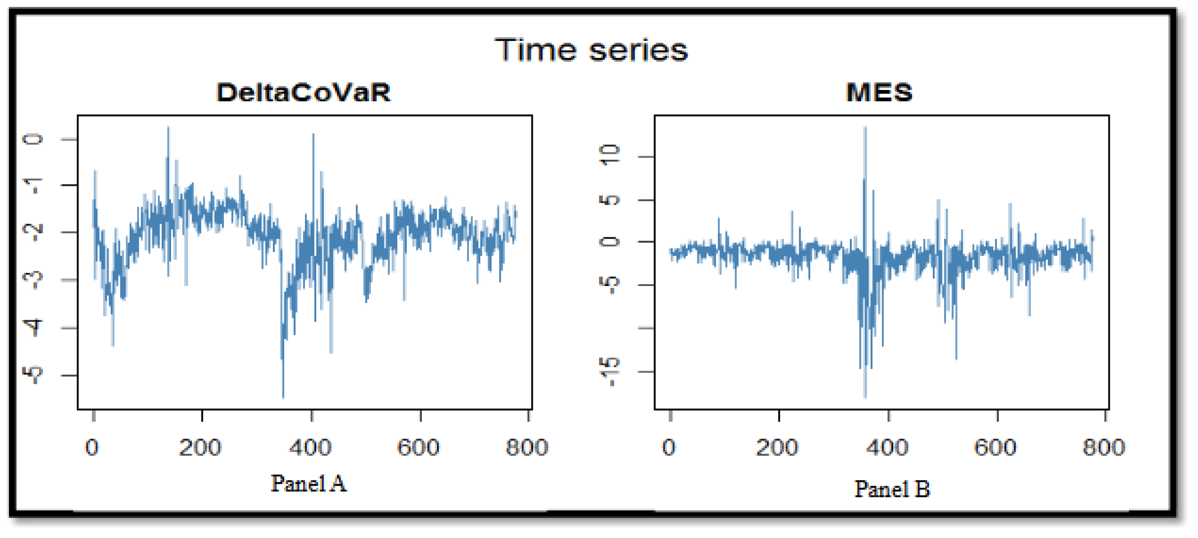An autoregressive structure AR(1) is implemented after detecting the presence of linear dependence in the residual series (see Figure 1). We also test the presence of any correlations in the squared residuals using the AFC. The results suggest the adoption of a GARCH(1,1) process. Therefore, the AR-GARCH(1,1) is used for systemic risk values (ΔCoVaR and MES) ranging from 2002 to 2015 in order to forecast their values for the next 12 months of 2016.27

4.3. Results and Discussion

In this section, we report the main results of our systemic risk measures, the results obtained after the implementation of the neural networks, the support vector machine, and the AR-GARCH fitting model. Also, we discuss the prediction accuracy and method performance.

First, we use the weekly28 stock returns to calculate the weekly systemic risk contribution and exposure measured by the ΔCoVaR and MES, respectively, for each bank of the sample.

Table 2. Systemic risk summary statistics. This table provides the summary statistics for the systemic risk measures used in our study. The sample consists of 134 European banks during the 2002–2016 period.

	∆CoVaR	MES
	Definition: The mean of weekly ∆CoVaRs is defined as the difference between the VaR of the system when the institution is at the 1% percentile and the VaR of the system when the institution is at its median (50% percentile) (%). Source: Bloomberg, own. calc.	Definition: The mean of weekly MESs is defined as the return of the institution when the system is at its 1% percentile worst days (%). Source: Bloomberg, own. calc.
Mean	−2.105	−2.771
Median	−1.329	−0.849
Standard deviation	4.169	7.177
Minimum	−8.427	−18.320
Maximum	3.675	11.955
Number of observations	2010	2010

reports the summary statistics of the ΔCoVaR and the MES, noting that the descriptive statistics are calculated on a yearly basis. The data consists of 134 banks with 2010 observations on the 2002–2016 period29. The mean of the ΔCoVaR is about −2.105, which implies that, on average, when the bank is at its 1% VaR, it increases the 1%VaR of the system by 2.105% during the 2002–2016 period. The minimum of the ΔCoVaR is about −8.427 and the maximum is about 3.675, with a standard deviation of 4.169, indicating that the systemic risk contribution measure in our study is relatively dispersed. As for the systemic risk exposure, the average of the MES is about −2.771%, meaning that, on average, the loss of each bank during the 2002–2016 period is about 2.771% when the system experiences its worst 1% times.

Table 3. Distribution of observations by year. This table shows the average of the systemic risk measures, ΔCoVaR and MES, for each year from 2002 to 2016.

Year	ΔCoVaR	MES
2002	−2.701	−3.071
2003	−2.320	−1.778
2004	−1.761	−1.393
2005	−1.448	−0.949
2006	−1.537	−1.896
2007	−1.690	−2.932
2008	−2.692	−6.892
2009	−2.452	−3.965
2010	−2.303	−2.858
2011	−2.381	−5.792
2012	−2.152	−1.996
2013	−1.866	−0.979
2014	−1.176	−1.907
2015	−2.079	−2.935
2016	−3.028	−2.235

lists the average systemic risk contribution and exposure for each year. The results show that systemic risk contribution was higher in crisis periods. The ΔCoVaR was around −2.7% in 2002 (the introduction of the Euro as the single currency of the European Union), around −2.6% during the 2007–2009 period (the global financial crisis), and around −2.3% during the 2010–2011 period (the European sovereign debt crisis) and in 2016 (Greece’s sovereign debt crisis). Similarly, the systemic risk exposure, MES, reaches its maximum value, −6.892%, during the year 2008 (the global financial crisis). The MES was also relatively high (−5.792%) during the European debt crisis of 2011.

Table 4. Distribution of observations by country. This table shows the average of the systemic risk measures, ΔCoVaR and MES, for each country of the sample.

Country	ΔCoVaR	MES
Austria	−1.113	−1.866
Belgium	−2.345	−2.274
Denmark	−1.158	−1.392
Finland	−1.079	−2.167
France	−1.273	−2.461
Germany	−2.299	−2.473
Greece	−4.321	−5.375
Ireland	−3.414	−5.926
Italy	−2.314	−3.530
Netherlands	−1.563	−3.763
Norway	−1.343	−1.485
Portugal	−2.411	−1.041
Spain	−2.276	−2.300
Sweden	−0.934	−3.416
Switzerland	−1.274	−2.279
United Kingdom	−1.992	−2.596

reports the average of the systemic risk contribution and exposure for each country. The results show that systemic risk contribution and exposure were relatively high in countries like Greece and Ireland.

After estimating the systemic risk measures using the ΔCoVaR and MES for all banks of the sample for the 2002–2016 period, we split the observations into three sets: from January 2002 to June 2012 (70% of the data for training) to train and implement the networks, from July 2012 to August 2014 (15% of the data for validation) to validate the model, and from September 2014 to December 2016 (15% of the data for testing) to test the accuracy of the artificial neural network and the support vector.

Table 5. Systemic risk forecasting results. This table reports the average of actual and forecasted values of systemic risk contribution (ΔCoVaR) and exposure (MES).

	Panel A: ΔCoVaR					Panel B: MES
	Actual	ANN		SVM	AR-GARCH	Actual	ANN		SVM	AR-GARCH
Month		1 Hidden Layer	2 Hidden Layers				1 Hidden Layer	2 Hidden Layers
January	−2.983	−2.172	−3.142	−2.825	−1.404	−1.367	−1.462	−1.497	−2.210	−1.531
February	−3.713	−2.274	−3.603	−2.859	−1.342	−1.197	−1.118	−1.089	−2.088	−1.618
March	−3.064	−2.145	−3.379	−3.138	−1.318	0.1953	0.095	−0.250	−2.067	−1.650
April	−2.941	−2.152	−3.338	−3.173	−1.308	−1.777	−1.678	−1.543	−2.237	−1.661
May	−2.997	−2.072	−3.328	−3.099	−1.304	−0.216	−0.366	−0.289	−2.154	−1.665
Jun	−3.035	−2.067	−3.173	−2.971	−1.302	−2.917	−2.998	−2.881	−2.269	−1.667
July	−2.346	−2.280	−3.117	−2.957	−1.301	0.820	0.737	0.775	−2.290	−1.652
August	−3.105	−2.165	−3.419	−3.488	−1.300	−5.655	−5.603	−5.813	−2.119	−1.680
September	−2.987	−1.499	−3.379	−3.298	−1.310	−3.972	−3.293	−3.397	−2.277	−1.368
October	−2.983	−2.022	−3.359	−3.233	−1.209	−3.678	−3.529	−3.569	−2.309	−1.599
November	−3.101	−2.060	−3.269	−3.100	−1.023	−6.043	−5.729	−5.570	−2.201	−1.781
December	−3.091	−2.086	−3.118	−2.982	−1.169	−1.013	−0.005	−0.057	−2.456	−1.038
Mean	−3.028	−2.082	−3.300	−3.093	−1.274	−2.235	−2.079	−2.098	−2.223	−1.575
A-MAPE		82.11%	11.504%	10.267%	57.932%		15.224%	13.019%	112.147%	109.563%

compares the mean values of the ΔCoVaR and MES predicted using the one and two hidden layer ANNs, the SVM, and the AR-GARCH(1,1), with the estimated values of the ΔCoVaR and MES calculated using the quantile regression and Equation (4), respectively.

To estimate the accuracy of each method, we estimate the adjusted error of the methods using the A-MAPE defined in Equation (9). Table 5 reports the forecasted values of the two systemic risk measures for the last 12 months of the sample period: from January 2016 to December 2016. As mentioned before, the actual values of the systemic risk contribution (ΔCoVaR) and exposure (MES) of the 2016 year are not included in the architectures of the neural networks (with one and two hidden layers) nor in the support vector machine or GARCH specification in order to test the efficiency of these methods in forecasting their values.

Panel A in Table 5 reports the results of the systemic risk contribution. The results show that the artificial neural network does not perform in the same way using one and two hidden layers. While the adjusted error (A-MAPE) of the value forecasted via one hidden layer is about 82.11%, the two hidden layer neural network performs better, with an adjusted error of 11.5%. The support vector machine also presents an effective performance, having an error of 10.267% only. While the AR-GARCH(1,1) specification model forecast values with a 57.932% error rate, it may be considered better than the one hidden layer neural network. This result suggests that the neural network architectures may not always capture the volatility among the observations, and choosing the number of hidden layers may be an important issue in this case.

The forecasting results of the systemic risk exposure are reported in Panel B in Table 5.

The results show that, despite the little difference in the error rates, again, the artificial neural network performs better when we use two hidden layer architectures. The error rates were 15.224% and 13.019% for one hidden layer and two layers, respectively. In contrast, the support vector machine and the AR-GARCH models fail to efficiently forecast the systemic risk measures of our sample.30

Briefly, our results show that the artificial neural networks are effective tools in predicting systemic risk contribution and exposure, as their mean error terms were 10.26% and 15.224%, and they outperform other prediction tools. Our results also show that while the support vector machine performs efficiently using the systemic risk contribution values, it miss-predicts the values of the marginal expected shortfall.

5. Conclusions and Discussion

This paper undertakes an empirical study on the prediction of systemic risk contribution and exposure in the European banking industry. Recognizing the increasing interconnectedness of financial institutions, especially banks, the study aims to develop robust tools for forecasting systemic risk—an essential step for mitigating potential financial crises. We proceed with a three-step methodology to forecast the systemic risk in European banks. First, we estimate the systemic risk contribution and exposure for 134 banks in 16 European countries during the 2002–2016 period. We use the delta conditional value at risk (ΔCoVaR), which measures the incremental risk a specific institution poses to the financial system under stress conditions, and the marginal expected shortfall (MES) to quantify systemic risk exposure, reflecting how much a bank is expected to lose during systemic events. These two measures, respectively, account for systemic risk contribution and exposure.

Next, the second step involves the application of four predictive modeling techniques to forecast the evolution of systemic risk over the final 12 months of the sample period. We implement two artificial neural networks (ANNs) with one and two hidden layers, a support vector machine (SVM), and autoregressive conditional heteroscedasticity (GARCH) to forecast the systemic risk for the last 12 months of the sample period. While ANN models can capture complex, non-linear relationships in data, the SVM is included for its robustness in classification and regression tasks, and the GARCH model is employed as a benchmark given its historical usage in volatility and risk modeling.

Finally, in the last step, we test the effectiveness of each forecasting approach by comparing the predicted values of systemic risk against the observed measured values. We estimate the performance level of each method using the adjusted mean absolute percentage error (A-MAPE), which accounts for potential bias and scale differences in prediction accuracy.

The empirical results show that the artificial neural network with two hidden layers significantly outperforms the other techniques, achieving a forecasting error rate between 10.26% and 15.22%. This suggests that deeper neural architectures are better equipped to model the complex dynamics underpinning systemic risk. Conversely, the support vector machine exhibits variable performance and does not consistently yield accurate predictions across the dataset. The GARCH model demonstrates the weakest performance, highlighting the limitations of traditional econometric models in identifying irregular interactions and severe risk events in financial turbulence.

As artificial intelligence and machine learning technologies rapidly advance and expand in use and applications, this study suggests that ANNs demonstrate good potential for addressing the challenge of systemic risk in banking and financial services. These findings emphasize the growing relevance of artificial intelligence and machine learning techniques in the domain of financial risk management. Specifically, the superior performance of ANN models suggests that such tools could play a pivotal role in the development of forward-looking systemic risk monitoring systems. Banking authorities and regulators may build upon these results to develop and refine systemic risk forecasting models, which would serve toward providing early warning indicators of banking distress, thereby possibly being able to implement corrective measures early on, and, consequently, minimizing systemic risk-associated costs and negative externalities in the economy as a whole.

The study’s findings have several important implications for understanding and managing systemic risk in the European banking sector from both economic and financial perspectives.

First, the outperformance of the artificial neural network (ANN), particularly with deeper architectures, for instance, two hidden layers, in terms of accuracy reflects the complex, non-linear nature of systemic risk in the financial systems and specifically in banks. This result shows that the systemic risk is not driven by linear interactions or simple volatility dynamics; rather, it arises from highly interdependent exposures, contagion effects, circular causality, and behavioral responses to stress.

The relatively low prediction error (10.26% to 15.22%) of the two hidden layers ANN suggests that deep learning models can be used to predict early stages of systemic instability. By adopting these models, regulators could monitor the evolving risk profile of banks and financial systems in near real time, allowing for earlier intervention and risk containment.

While the ANN with two hidden layers shows high performance in predicting systemic risk, the SVM did not effectively quantify it. The results of this study show that the error was relatively high and that the predicted values did not consistently match the actual ones. The reason is that the SVM, a margin-based classifier, can capture a relatively stable and separable relationship between the inputs and the outputs. This relationship is absent in the case of systemic risk, where the market is rapidly shifting and the conditions are unstable.

These results are consistent with the fact that during systemic events when correlations between asset returns rise, defaults become more concentrated and liquidity dries up, and complex dynamics become difficult to model accurately using traditional approaches.

The results also show that the GARCH model, a standard model is forecasting volatility, performed the worst in predicting systemic risk. This finding is economically well-founded. GARCH models capture time-varying volatility with a relatively stable structure in the data, and they are thus unable to capture tail dependencies and cross-sectional linkages in financial markets.

More generally, when systemic risk arises, what matters is not only the volatility of an individual bank or specific sector in the market but rather how distress propagates across institutions and maybe countries. This characteristic is missed in GARCH models, which treat each entity in isolation, neglecting the conditional dependence structures between institutions.

This evidence aligns with the prevailing perspective in financial economics. While GARCH remains useful for modeling market risk, it is insufficient for measuring systemic risk, which is characterized by complex interdependencies and multidimensional relationships.

From a macroprudential policy perspective, the results of this study suggest that traditional risk models may be unable to detect and predict systemic threats in real time. Conversely, AI-driven models with deep learning architectures, like ANNs, can offer a more effective approach to the early detection and management of financial instability. It is essential for central banks and regulatory authorities to undertake preventive policies such as liquidity support, capital requirements adjustments, or resolution planning.