A Hybrid Forecasting Model for Stock Price Prediction: The Case of Iranian Listed Companies

Abstract

This paper introduces advanced computational methods for stock price prediction, integrating Fast Recurrent Neural Networks (FastRNN) with meta-heuristic algorithms such as the Horse Herd Optimization Algorithm (HOA) and the Spotted Hyena Optimizer (SHO). By challenging the Efficient Market Hypothesis (EMH) and Random Walk Hypothesis, our research demonstrates the effectiveness of these hybrid models in semi-strong or weak-form efficient markets. The study leverages data from five listed Iranian companies (2011–2021) and 25 factors encompassing technical, fundamental, and economic considerations. Our findings highlight the superior accuracy of the FastRNN optimised by HOA, SHO, and a Generative Adversarial Network (GAN) in forecasting stock prices compared to conventional FastRNN models. This research contributes to the multidisciplinary field of computational economics, emphasising advanced computing capabilities to address complex economic problems through innovative econometrics, optimisation, and machine learning approaches.

1. Introduction

Anticipating stock market movements remains a formidable challenge due to the non-parametric, non-linear, and non-stationary nature of stock prices (Abu-Mostafa & Atiya, 1996). This complexity is exacerbated by macroeconomic variables, industry dynamics, firm-specific factors, and investor psychology (Daniel et al., 2002; Laopodis, 2011; Peiro, 2016). Traditional statistical models (e.g., ARIMA, logistic regression) and operations research methods (e.g., linear programming) often fail to capture these dynamics because they rely on restrictive assumptions, such as linear relationships and stationary data—conditions rarely met in real-world markets (Beckwith, 2001; Chang et al., 2004). So, this represents a research gap in the literature and motivates further studies to offer a more capable model.

Artificial intelligence (AI) techniques, particularly neural networks, have emerged as promising alternatives due to their ability to model non-linear patterns without rigid assumptions (Chen et al., 2003; Affenzeller et al., 2009). For instance, recurrent neural networks (RNNs) and long short-term memory (LSTM) models excel at processing sequential data but suffer from computational inefficiency, gradient instability, and reliance on large labelled datasets (G. Zhang et al., 1998; Nabipour et al., 2020). Similarly, while generative adversarial networks (GANs) mitigate data scarcity issues through semi-supervised learning, their training dynamics (e.g., mode collapse, discriminator-generator imbalance) often lead to suboptimal performance in financial time-series forecasting (X. Zhou et al., 2018; K. Zhang et al., 2019).

Given the above we can identify two critical limitations regarding the current techniques, which represent a Research Gap in the literature and the Motivation for the current study, as follows: Training Instability and Hyperparameter Sensitivity. In terms of Training Instability we can argue that classical RNNs struggle with vanishing gradients and high computational costs, especially in volatile markets (Yadav et al., 2021). In terms of Hyperparameter Sensitivity, we can refer to existing hybrid models (e.g., LSTM-GAN) that require extensive tuning of hyperparameters, which is often ad hoc and computationally expensive (Koochali et al., 2019).

To address these gaps, this study introduces a FastRNN model enhanced with residual connections and two trainable parameters (α and β), stabilising gradients and reducing computational overhead compared to traditional RNNs (see Equations (12) and (13)). We further integrate meta-heuristic algorithms—the Horse Herd Optimization Algorithm (HOA) and the Spotted Hyena Optimizer (SHO)—to automate hyperparameter tuning, addressing the sensitivity issue. Finally, we adopt a GAN framework with LSTM as the generator to leverage unlabelled data, improving robustness in low-data regimes (e.g., emerging markets like Iran).

By marrying FastRNN’s temporal stability with GANs’ data efficiency and meta-heuristics’ optimisation intelligence, we overcome the trilemma that has constrained emerging market forecasting: our model maintains gradient coherence through market shocks, autonomously adapts hyperparameters via HOA/SHO algorithms, and leverages unlabelled data through adversarial regularisation. When validated on Iran’s Tehran Stock Exchange—using 2000+ data points across five companies—the results demonstrate how architectural synthesis can conquer problems that isolated approaches cannot.

The remainder of the paper is structured as follows: Section 2 reviews related work; Section 3 and Section 4 detail the methodology and data; Section 5 presents results; and Section 6 concludes.

2. Literature Review

The financial viewpoint of organisations remains a primary focus of current research (Askarany et al., 2024; Eghbal et al., 2023). That is probably why forecasting stock prices remains a central concern in finance, due to financial markets’ inherent complexity and chaotic behaviour. The literature on stock market prediction has evolved from classical statistical techniques to sophisticated machine learning and hybrid artificial intelligence (AI) models. This review critically synthesises the contributions and limitations of existing approaches, identifies key studies, and defines the research gap this paper seeks to address.

2.1. Early Approaches: Statistical and Econometric Models

Classical methods such as ARIMA, exponential smoothing, and Box–Jenkins models (Naylor et al., 1972) were among the earliest tools applied in financial forecasting. These methods assume stationarity and linearity—conditions seldom satisfied in real-world markets, limiting their ability to handle non-linear dependencies, regime shifts, and investor sentiment fluctuations (Beckwith, 2001; Peiro, 2016). Although interpretable and straightforward to implement, their performance deteriorates under the volatile or noisy conditions typical of emerging markets.

Key limitation: inflexibility to model complex, non-linear relationships in high-frequency data.

2.2. Emergence of Soft Computing and Neural Networks

The limitations of statistical models prompted a shift toward AI-based techniques. Neural networks (Zekić-Sušac, 1998; Enke & Thawornwong, 2005), fuzzy logic (Carlsson & Fullér, 2009), and support vector machines (Tay & Cao, 2001) became popular for their ability to model non-linearities without rigid assumptions. Deep learning architectures, particularly recurrent neural networks (RNNs) and long short-term memory (LSTM) models, demonstrated superior capabilities in capturing sequential dependencies (G. Zhang et al., 1998; Chong et al., 2017).

However, these models introduced new challenges. RNNs suffer from vanishing gradients, limiting long-term memory retention. LSTMs require large, labelled datasets and extensive hyperparameter tuning, which is computationally expensive and often impractical in data-sparse environments like Iran (Nabipour et al., 2020).

Key limitations: high training costs, gradient instability, and dependence on large, labelled datasets.

2.3. Hybrid and Meta-Heuristic Models

Recent studies have integrated hybrid AI models to mitigate individual algorithmic weaknesses. GANs have been applied to generate synthetic data and reduce training dependence on labelled samples (X. Zhou et al., 2018; K. Zhang et al., 2019). Meta-heuristic optimisation techniques such as Particle Swarm Optimisation (PSO), Artificial Bee Colony (Shah et al., 2018), and the Spotted Hyena Optimizer (Dhiman & Kumar, 2017) have been used to fine-tune model parameters.

While these efforts show promise, they often suffer from instability (e.g., GAN mode collapse), manual tuning, or limited validation on non-stationary financial time series (Koochali et al., 2019; K. Zhou et al., 2020). Furthermore, many hybrid models lack a coherent framework that combines temporal stability, computational efficiency, and adaptability to sparse data regimes.

Key limitation: fragmented improvements without a unified architecture can address all three core issues—gradient instability, hyperparameter sensitivity, and data scarcity.

2.4. Identification of the Research Gap

Although previous models have contributed significantly to forecasting accuracy, several gaps remain:

• Gradient-Stable Temporal Modelling: Traditional RNNs lack robustness in turbulent financial environments, and few studies implement gradient-stabilising architectures such as FastRNN (Yadav et al., 2021).
• Efficient Hyperparameter Optimisation: Most hybrid models rely on manual or static tuning, with minimal focus on biologically inspired optimisation for dynamic, high-dimensional search spaces.
• Semi-Supervised Learning in Low-Data Regimes: GANs have been adapted for financial forecasting. However, few models successfully combine adversarial learning with temporal deep networks in markets with limited labelled data (e.g., Iran).
• Lack of Integration: To date, no model has simultaneously integrated a FastRNN for temporal coherence, meta-heuristic algorithms for hyperparameter tuning, and GANs for semi-supervised learning within a single framework.

2.5. Contribution of the Present Study

This study bridges the above gaps through a novel hybrid model that integrates:

• FastRNN with residual connections, offering gradient stability and reduced computational cost.
• The Horse Herd Optimization Algorithm (HOA) and the Spotted Hyena Optimizer (SHO), enabling efficient hyperparameter tuning.
• GAN architecture with an LSTM generator, allowing robust learning from limited and noisy datasets.

Unlike earlier models that focused narrowly on individual techniques (e.g., Zekić-Sušac, 1998 on MLPs or K. Zhang et al., 2019 on GANs), this research proposes a unified architecture suitable for semi-efficient and volatile markets such as Iran’s Tehran Stock Exchange. It also provides empirical evidence across multiple firms, demonstrating improved forecasting accuracy (MAPE < 20%) and reduced training instability. These unresolved challenges motivate our investigation of FastRNN’s residual architecture combined with meta-heuristic optimisation. We employ a dataset of five Iranian companies (2011–2021) to test these questions with 25 input variables, as detailed in the next section.

3. Methodology

This study employs an analytical mathematical research methodology. It uses data from five companies listed on the Tehran Stock Exchange between 2011 and 2021. Our sample comprises a panel of firms listed on the Tehran Stock Exchange (TSE). The TSE’s data are based on audited financial statements and board reports, a reliable source of information used by many authors (Pouryousof et al., 2022).

These companies have the maximum floating shares with maximum market efficiency in terms of price trend and are similar in size. Following K. Zhang et al. (2019) and Ronaghi et al. (2022), five listed companies are selected to facilitate pairwise comparison of the models and avoid computational complexity. These companies are coded from 1 to 5, and daily data are analysed for 11 years, as shown in

Table 1. Stock dataset and data count for each of the five domestic stocks.

Company	Data Count (for 11 Years)	Usable Sequences
a	2363	2355
b	2038	2030
c	2264	2256
d	2362	2354
e	2457	2449
Total	11,484	11,444

.

• Sample Selection

We analysed five companies listed on the Tehran Stock Exchange (TSE) from 2011–2021, selected through a stratified process:

• Criteria:

  ○

  Market Efficiency: Companies with floating shares ≥ 30% of total shares (TSE threshold for “high liquidity”).

  ○

  Size Homogeneity: Market capitalisation within $1–2 billion USD (2011 baseline) to control for size effects.

  ○

  Sector Representation: One company from the banking, petroleum, mining, pharmaceuticals, and automotive sectors—the five largest sectors by TSE trading volume.

2.

Rationale:

This selection ensures:

○

Liquidity: High floating shares reduce illiquidity bias in price trends.

○

Comparability: Similar sizes minimise volatility differences from capital structure effects.

○

Diversity: Sector coverage accounts for macroeconomic variability (e.g., oil price impacts on petroleum stocks).

Data Source: Company filings from the TSE Rahavard Novin Database (https://mabnadp.com/products/rahavard-novin, accessed on 8 August 2022), Iran’s official repository for audited financial data.

2.

Data Collection and Variables

The selected companies have high levels of pricing efficiency and free float, which reduces their susceptibility to manipulation and better reflects real market dynamics. The floating share ratio is commonly used as a proxy for liquidity and market depth, particularly in emerging nations.

The sample of five firms was selected through a multi-criteria filtering process designed to ensure data quality, homogeneity, and relevance for time series modelling with deep learning techniques. Specifically, the firms were chosen based on the following quantitative and qualitative criteria:

• Free Float Ratio: We prioritised firms with the highest free-floating shares on the TSE to ensure sufficient liquidity and minimise price manipulation effects. High-float shares tend to reflect market-driven price dynamics better.
• Market Efficiency Indicators: Using historical return autocorrelation and Hurst exponent estimation, we selected firms exhibiting near-random walk behaviour in returns, indicative of high market efficiency and suitable for modelling with stochastic and learning-based methods.
• Size and Capitalisation Homogeneity: We constrained the sample to firms within a narrow band of market capitalisation (±15%) to minimise size-related heteroskedasticity in return behaviour and model error variance.
• Data Completeness: Firms with fully available and uninterrupted daily trading records from January 2011 to December 2021 were included to support long-sequence forecasting and reduce data imputation noise.
• Sample Size Justification: Following K. Zhang et al. (2019) and Ronaghi et al. (2022), five listed companies were selected to facilitate pairwise comparison of forecasting models while keeping the computational complexity manageable. This also allows for consistent benchmarking of model performance across firms.

The dataset used in this study was compiled from the following widely recognised and reliable sources in the context of Iranian capital market research:

• Codal.Ir: Operated by the Securities and Exchange Organization of Iran, Codal serves as the official repository for audited financial statements, corporate disclosures, and regulatory filings of publicly listed firms.
• TSETMC.com (Tehran Securities Exchange Technology Management Co., Tehran, Iran): This is the authoritative platform for intra-day and historical trading data, including price, volume, order book depth, and technical indicators for all TSE-listed companies.
• Rahavard365: A well-established commercial financial data provider used extensively in academic and industry contexts. It is beneficial for retrieving computed technical indicators such as RSI, MACD, Bollinger Bands, and moving averages.
• Central Bank of Iran: Used for obtaining macroeconomic variables such as exchange rates (e.g., the USD/IRR rate), inflation, and monetary indicators, aligned with prior studies on macro-financial forecasting in Iran.
• WTI Crude Oil Price and Gold Price (per ounce): Both series were sourced from tgju.org, which provides daily updates on international commodity prices in a format commonly used by financial analysts and academic researchers in Iran.

3.1. Dataset

Following Yadav et al. (2021), who called for the inclusion of external factors in stock price forecasting, and by reviewing prior research (e.g., Dastani Heriss et al., 2020; Zeng, 2020; Li et al., 2022), a total of 25 variables are considered as the inputs for the proposed model, and they are divided into three categories:

• Fundamental components: EPS, DPS, price-to-earnings ratio, firm size, and return on assets;
• Technical components: closing price, low price, high price, trade value, overall index, trade volume, opening price, last price, relative strength index, moving average (MA) (at 26, 12, and 5 days), MA convergence/divergence, exponential MA (at 12 and 26 days), and the number of pre-opening trades;
• Macroeconomic components include the exchange rate, West Texas Intermediate crude oil price, gold per ounce, and inflation rate.

Data for the above components are collected from reliable databases, with annual and monthly data converted to daily data in EViews Version 12 and used as inputs for the FastRNN and GAN models. Finally, two meta-heuristic algorithms, i.e., HOA and SHO, are integrated into the FastRNN. Daily data are used as input for the model, so the prices are forecast for the next day (next trading session). The proposed models are coded using Python (3.9.0) and Jupyter Notebooks V7 in Google Colab with 25 GB of RAM and GPU for increased processing speed.

The FastRNN and GAN models are also designed and implemented on the TensorFlow and Keras platforms. The HOA and SHO meta-heuristic algorithms are directly implemented in a Python environment, without any particular library, and then integrated into the FastRNN. Data are normalised using min-max normalisation. In total, 9110 pieces of final stock price data are analysed for the five companies, with 90% of the data selected for training and the remaining 10% used for testing.

We analyse the daily closing prices of five publicly traded companies over 11 years (2011–2021). Each dataset includes 25 empirically validated technical and financial indicators selected for their demonstrated predictive relevance. Our modelling framework adopts a rigorous rolling-window strategy. At each step, a contiguous 7-day block of multivariate observations (input shape: [7 × 25]) is used to forecast the closing price of the following trading day. This window advances sequentially through the dataset, yielding 11,444 training sequences from the original 11,484 observations while strictly maintaining temporal order—terminating one step before the dataset’s end to ensure the availability of target values for validation.

Model performance is evaluated using mean squared error (MSE), serving as the primary metric for assessing prediction accuracy and as a feedback mechanism for iterative parameter optimisation. Specifically, least-squares-derived coefficients are employed to correct systematic forecasting biases. The data are split into 90% training (10,300 sequences) and 10% testing (1144 sequences) to ensure rigorous model assessment. All models are trained using a fixed batch size 32, balancing computational efficiency with gradient stability.

3.2. Models

The models used in this research are GAN, FastRNN, and the hybrid FastRNN optimised by HOA and SHO. First, following K. Zhang et al. (2019), the deep learning model is presented for predicting the closing price of daily transactions. This is a novel GAN architecture with the LSTM as the generator and the MLP as the discriminator. This model is trained to predict the daily closing price with stock data from the past few days.

3.3. GAN

The GAN architecture was introduced by Goodfellow et al. (2014) as a means of generating realistic images. GAN is developed based on a zero-sum game with two deep learning networks: the generator and the discriminator. As the word adversarial suggests, the generator and the discriminator play a minimax game against each other. The generator outputs synthetic data, while the discriminator evaluates them as real or fake. During training, the generator aims to increase the discriminator’s error rate. In other words, the more mistakes the discriminator makes, the better the generator performs. The goal of the discriminator is to reduce its error rate. In each iteration, both networks move towards their goals using gradient descent. The generator tries to fool the discriminator, while the discriminator tries to avoid being misled. Eventually, the data (e.g., images, audio, video, and time series) drawn from the generator can fool even the most sophisticated discriminator.

3.4. Generator

The generator follows unsupervised learning that automatically discovers patterns or anomalies in the data. The generator aims to learn how to generate new samples with the same data as the training set. During the training phase, the generator performs density estimation whereby it learns to estimate an unobservable probability density function (G) based on observed data. It must be noted that the generator not only copies existing samples but also generates new samples from a distribution.

The generator of the proposed model is designed using LSTM due to its ability to process time series data. Future closing price is predicted from the data for the last 11 years using seven financial parameters—high and low price, closing price, overall index, trade value, trade volume, and five-day MA (MA5)—in conjunction with the leaky rectified linear unit (Leaky ReLU) activation function and dropout.

A set of daily stock data for year t is as follows:

$$\begin{gathered} X=x_1+x_2+\dots +x_t \\ {\left[X_{k,i}\right]}_{i=1}^7=\left[X_{k,High},X_{k,Low},X_{k,Close},X_{k,Overall\_Index}{X}_{k,Value},X_{k,Volume},X_{k,MA5}\right] \end{gathered}$$

(1)

Through the generator, the output $h_t$ is extracted from the LSTM and imported into a fully connected layer with seven neurons to produce ${\widehat{x}}_{t+1}$. ${\widehat{x}}_{t+1}$ is generated as an approximation of $x_{t+1}$, and ${\widehat{x}}_{t+1.close}$ can be used as a forecast of the ${\widehat{x}}_{t+1}$ closing price received on day $t+1$. The output of the generator G(X) is defined as follows:

$$h_t=g\left(X\right)$$

(2)

$$G\left(X\right)={\widehat{x}}_{t+1}=\delta \left(W_h^T{h}_t+b_h\right)$$

(3)

where $g\left(·\right)$ is the output of the LSTM and $h_t$ is the output of the LSTM with $X=\{x_1,x_2,\dots ,x_t\}$ as the input; $\delta$ denotes the Leaky ReLU activation function; and $W_h^T{h}_t$ and $b_h$ denote weight and bias, respectively, in the fully connected layer. Thus, with ${\widehat{x}}_{t+1}$ and $X$, we can continue to forecast ${\widehat{x}}_{t+2}$.

3.5. Discriminator

The task of the discriminator is to create a differentiable function (D) that can be used to classify the data. The discriminator should be 0 when fake data are entered and 1 when real data are entered. We use the MLP as the discriminator, with three hidden layers, H1, H2, and H3, consisting of 72, 100, and 10 neurons, respectively. Leaky ReLU is the activation function for the hidden layers, while the output layer uses the sigmoid function. In addition, the MLP is optimised using cross-entropy loss as the loss function. More specifically, $X=\{x_1,x_2,\dots ,x_t\}$ is concatenated with ${\widehat{x}}_{t+1}$ to obtain $\{x_1,x_2,\dots ,x_t,x_{t+1}\}$ as the fake data $X_{fake}$. The same is done with $X=\{x_1,x_2,\dots ,x_t\}$ and $x_{t+1}$ to get $\{x_1,x_2,\dots ,x_t,x_{t+1}\}$ as the real data $X_{real}$. The output of the discriminator is as follows:

$$D\left(X_{fake}\right)=\sigma \left(d\left(X_{fake}\right)\right)$$

(4)

$$D\left(X_{real}\right)=\sigma \left(d\left(X_{real}\right)\right)$$

(5)

where $d(·)$ is the output of the MLP and the sigmoid function. Both $X_{real}$ and $X_{fake}$ output a single scalar.

3.6. Proposed GAN Architecture

The architecture of the proposed GAN uses the two models mentioned above. According to Goodfellow et al. (2014), both G and D try to optimise a value function in the two-player minimax game. Similarly, the optimisation of the value function $V(G,D)$ is defined as follows:

$$\underset{G}{min}\underset{D}{max}V\left(G.D\right)=E\left[\log D\left(X_{real}\right)\right]+E\left[\log 1-D\left(X_{fake}\right)\right]$$

(6)

$$D_{loss}=-{\displaystyle \frac{1}{m}}\sum _{i=1}^m\log D\left(X_{real}^i\right)-{\displaystyle \frac{1}{m}}\sum _{i=1}^m\mathrm{l}\mathrm{o}\mathrm{g}(1-D(X_{fake}^i))$$

(7)

$$g_{MSE}={\displaystyle \frac{1}{m}}\sum _{i=1}^m({\widehat{X}}_{t+1}^i-X_{t+1}^i{)}^2$$

(8)

$$g_{loss}={\displaystyle \frac{1}{m}}\sum _{i=1}^m\mathrm{l}\mathrm{o}\mathrm{g}(1-D(X_{fake}^i))$$

(9)

$$G_{loss}={\lambda }_1{g}_{MSE}+{\lambda }_2{g}_{loss}$$

(10)

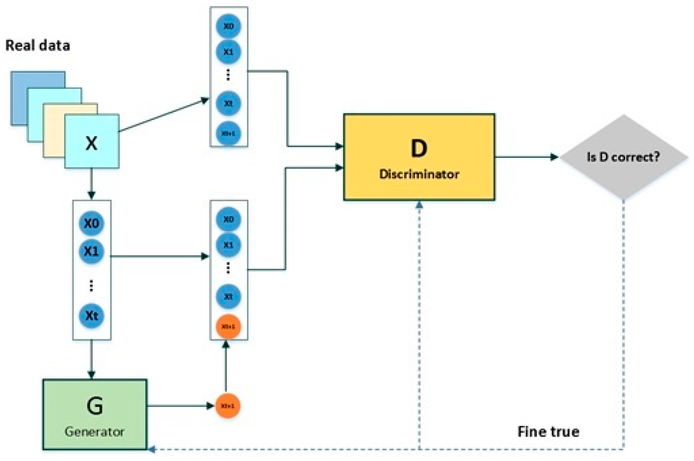
The loss function $G_{loss}$ is a combination of $g_{MSE}$ and $g_{loss}$ with the hyperparameters ${\lambda }_1$ and ${\lambda }_2$ set by the Adam algorithm. Figure 1 shows the proposed GAN architecture. The rationale for using $X_{real}$ and $X_{fake}$ instead of $x_{t+1}$ and ${\widehat{x}}_{t+1}$ in the discriminator is that we expect the discriminator to capture the correlation and time series information between $x_{t+1}$ and $X$.

The FastRNN model adapted from Yadav et al. (2021) and the meta-heuristic algorithms (HOA and SHO) are described next.

The proposed adversarial architecture for financial time-series generation is shown in Figure 1. It consists of three main parts: (1) a two-layer LSTM generator (128 units per layer, LeakyReLU activation with α = 0.2) that converts seven input technical indicators into temporally coherent synthetic price sequences; (2) a three-layer multilayer perceptron (MLP) discriminator (layer sizes: 72–100–10) that ends in a sigmoid activation to separate generated from real data probabilistically; and (3) a composite loss function that weighs adversarial challenge and reconstruction fidelity, with adversarial loss at 30% and mean squared error (MSE) at 70%. The asymmetric structure of the architecture pairs feedforward discrimination with recurrent generation to enforce realistic market behaviour while ensuring training stability through gradient clipping (threshold ± 1.0) and batch normalisation, and training continues until a Nash equilibrium is approximated, defined by discriminator accuracy convergent to 50 ± 2%.

3.7. FastRNN

FastRNN was proposed by Microsoft in 2018. This model is based on a residual network (ResNet), where the network layers are not stacked on each other. FastRNN uses residual connections from ResNet and provides stable training with comparable accuracies at much lower computational costs. Fast RNN forecasts are 19% more accurate than regular RNN and slightly less accurate than gated RNN.

Let $X=[x_1,x_2,\dots ,x_T]$ as the input vector, where $x_t\in R^D$ is the $t$-th step feature vector. For a multi-class RNN, the function $F:R^{DxT}1,\dots ,L$ is learnt and will forecast any of these L classes for a given point of data that is X.

In a regular RNN architecture, hidden state vectors are represented by the following equation:

$$h_t=tanh\left(W{x}_t+U{b}_{t-1}+b\right)$$

(11)

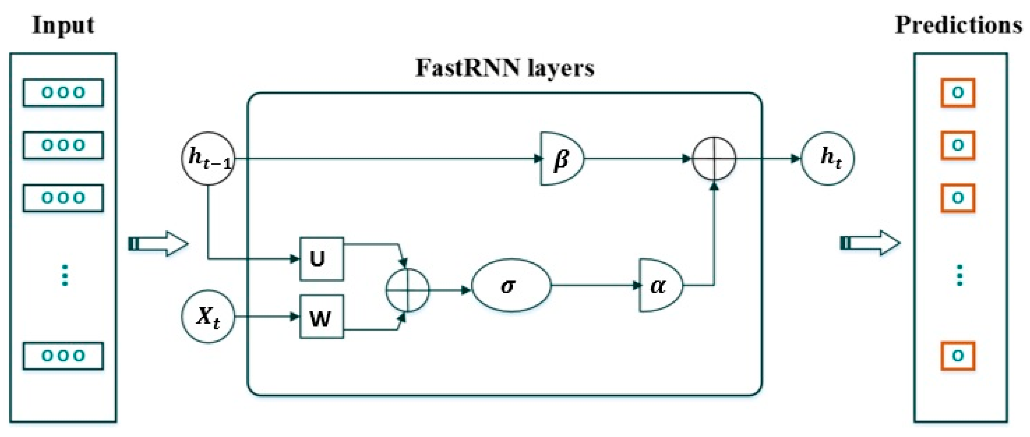
Training U and W in the above structure is difficult, since the gradient can have an exponentially large (in $T$) condition number. Unitary network-based solutions can address this problem by expanding the network size, but they become significantly larger during that process, and the model’s accuracy may suffer. However, FastRNN uses a simple weighted residual connection to stabilise the training by creating well-conditioned gradients. More specifically, it updates the hidden state $h_t$ as follows:

$${h^{\prime }}_t=\sigma \left(W{x}_t+U{h}_{t-1}+b\right)$$

(12)

$$h_t=\alpha {h^{\prime }}_t+\beta h_{t-1}$$

(13)

where $\alpha$ and $\beta$ are trainable weights parameterised by the sigmoid function and limited to the range $\alpha >0$ and $\beta <1$. $\sigma$ is a non-linear function such as a hyperbolic tangent, sigmoid, or ReLU activation function and can vary across datasets.

Unlike unitary methods, FastRNN does not introduce costly systemic constraints on U; hence, it scales well to massive datasets with typical optimisation methods. The proposed FastRNN-based model for stock market predictions is shown in Figure 2.

FastRNN systematically reconditions the hidden layer through $\alpha$ and $\beta$ by limiting the extent to which it is updated by the attribute vector $x_t$. Moreover, FastRNN has two more parameters than the regular RNN but only a fraction of its computational complexity. Unlike unitary methods, FastRNN imposes no costly systemic constraints on $U$. Therefore, it scales well to massive datasets with typical optimisation methods.

The proposed FastRNN for stock price forecasting is shown in Figure 2.

This study incorporates a time-series dataset from 2011 to 2021, encompassing daily observations of 25 factors influencing stock prices. The dataset is derived from five companies, where 90% of the data spanning 2011 to 2020 are allocated for training purposes, and the remaining 10% from 2021 are reserved for testing. An essential component of the Fast Recurrent Neural Network (FastRNN) and its hybrid counterpart, optimised by the Horse Herd Optimization Algorithm (HOA) and the Spotted Hyena Optimizer (SHO), is the activation function (Emami & Rafsanjani, 2024; Mehrabi et al., 2024; Yeganehmehr & Ebrahimnezhad, 2025). This research identifies the Leaky Rectified Linear Unit (ReLU) as the optimal activation function for the hidden state. Leaky ReLU’s widespread utilisation in neural networks is attributed to its desirable properties, including non-linearity and the absence of a constant derivative. Subsequently, the study employs two meta-heuristic algorithms, namely HOA and SHO, to fine-tune and optimise the hyperparameters of the FastRNN. The subsequent sections briefly elaborate on these meta-heuristic algorithms.

3.8. HOA

The Horse Herd Optimization Algorithm (HOA) emulates six fundamental aspects of horses’ social behaviour across various life stages: grazing, hierarchy, sociability, imitation, defence mechanisms, and roaming. Renowned for its efficacy in addressing intricate high-dimensional problems, this algorithm exhibits notable performance owing to its extensive set of control parameters. In the realm of high-dimensional global optimisation challenges, HOA stands out (Priya et al., 2024; Sharma et al., 2025; Si et al., 2025), demonstrating efficiency on par with other nature-inspired optimisation algorithms, including but not limited to the Grasshopper Optimization Algorithm, the Sine Cosine Algorithm (SCA), the Multi-Verse Optimizer (MVO), Moth-Flame Optimization, the Dragonfly Algorithm, and the Grey Wolf Optimizer (GWO).

3.9. SHO

Emerging as derivatives of natural phenomena, novel meta-heuristic algorithms offer innovative optimisation approaches. One such algorithm, the Spotted Hyena Optimizer (SHO), introduced by Dhiman and Kumar (2017), draws inspiration from the social behaviour of spotted hyenas. SHO initiates its process with a set of randomly generated solutions. Throughout each iteration, search agents dynamically adjust their positions using four operators: exploration (searching for prey), chasing target, encircling prey, and attacking prey (exploitation). The algorithm mirrors the behaviour of spotted hyenas as they identify and encircle prey. In the context of the hyena algorithm, each hyena’s position represents a potential solution to the optimisation problem, with the position of the most optimal hyena approximating the location of the prey. Hyenas, symbolising solutions, strategically encircle the prey (optimal resolution) in diverse states and scenarios, unveiling potential and more optimal solutions.

Recent investigations have indicated that SHO exhibits superior accuracy to other optimisation algorithms such as PSO, MVO, SCA, GWO, the Gravitational Search Algorithm, Harmony Search, and the Genetic Algorithm (Dhiman & Kumar, 2017). In the present study, SHO is employed to optimise FastRNN and is juxtaposed with HOA, known for its proficiency in addressing high-dimensional feature selection problems.

The following section uses the HOA and SHO meta-heuristic algorithms to optimise the proposed FastRNN following MiarNaeimi et al. (2021) and Dhiman and Kumar (2017).

3.10. Initialisation of the Proposed Models’ Parameters

Neural networks, including Deep Neural Networks (DNNs), are characterised by crucial hyperparameters, such as the number of layers, neurons in each layer, and the activation function, significantly influencing their performance. However, manually tuning these hyperparameters is often a protracted and laborious process. Consequently, the proposed FastRNN undergoes optimisation in this investigation through the Horse Herd Optimization Algorithm (HOA) and the Spotted Hyena Optimizer (SHO). Each meta-heuristic algorithm generates an initial population, adhering to predefined upper and lower bounds, and iteratively refines solutions based on their respective operators. It is imperative to highlight that the mean squared error (MSE) serves as the objective function for both HOA and SHO. Their parameters must be fine-tuned to facilitate a meaningful comparison of all proposed models, including FastRNN, FastRNN optimised by HOA, and FastRNN optimised by SHO and GAN. HOA and SHO parameters encompassing population size, number of iterations, and problem dimensions are uniformly configured to ensure equitable algorithmic comparison. Notably, GAN necessitates an extended number of iterations owing to its intricate structure, a subject expounded upon in subsequent sections.

Table 2. Parameters of HOA and SHO for FastRNN optimisation.

Algorithm	Parameter	Value
HOA	N Population	20
	Max Iteration	50
	Dimension	17
	W1	1
	phiD	0.02
	phiI	0.02
SHO	N Population	20
	Max Iteration	50
	Dimension	17
	Min	0.5
	Max	1

presents the parameters employed for optimising FastRNN by HOA and SHO.

The Horse Herd Optimization Algorithm (HOA) and the Spotted Hyena Optimizer (SHO) parameter settings were used to improve the architecture and hyperparameters of the FastRNN forecasting model in a 17-dimensional search space, as indicated in Table 2. Each dimension is associated with a unique model parameter, such as the number of layers, dropout rate, or independent weight values. For both HOA and SHO, the population size was fixed at 20 and the maximum number of iterations at 50, based on standard practice and empirical trials demonstrating dependable convergence within reasonable computational cost (Yang & Deb, 2014). The values in this table are fixed control parameters for the meta-heuristic algorithms selected to ensure convergence, stability, and fairness across comparative experiments.

Following the configuration validated by Jamal et al. (2024), the control parameters for the HOA algorithm were set to W1 = 1 and phiD = phiI = 0.2. This setup was carefully selected to balance exploration and exploitation effectively while maintaining stable and coherent herd dynamics throughout the optimisation process. The problem’s dimensionality was set to 17, corresponding precisely to the number of model parameters undergoing calibration. According to Dhiman & Kumar, 2017, whose configuration has shown strong performance in high-dimensional, non-linear search spaces, the randomness control parameters for the SHO algorithm were set to a minimum of 0.5 and a maximum of 1.0. All initial candidate solutions were randomly initialised within predefined upper and lower bounds for each hyperparameter, and optimisation was guided by the mean squared error (MSE), which was evaluated on a dedicated validation subset and used as the objective function. This design guarantees methodological rigour, complete reproducibility, and an objective optimisation process in all experimental settings.

As delineated in

Table 3. Parameters of the proposed model for stock price forecasting.

Algorithm	Parameter	Value
FastRNN_Base	Epochs	100
	Learning rate	0.001
	FastRNN layer	2
	Batch size	32
	Dropout	0.1
	Loss	MSE
FastRNN_HOA	Epochs	100
	Learning rate	0.001
	FastRNN layer	1–3
	Batch size	32
	Dropout	0–0.9
	Loss	MSE
FastRNN_HOA	Epochs	100
	Learning rate	0.001
	FastRNN layer	1–3
	Batch size	32
	Dropout	0–0.9
	Loss	MSE
FastRNN_SHO	Epochs	100
	Learning rate	0.001
	FastRNN layer	1–3
	Batch size	32
	Dropout	0–0.9
	Loss	MSE
GAN_Base	Epochs	1000
	Learning rate	0.001
	FastRNN layer	LSTM
	Batch size	32
	Dropout	0.3
	Loss	MLP-Dense

, uniformity is maintained in critical parameters—precisely the number of iterations, batch size, and loss function—across FastRNN_Base, FastRNN_HOA, and FastRNN_SHO, ensuring a robust basis for comparison. Notably, within FastRNN_HOA and FastRNN_SHO, specific parameters, including the number of FastRNN layers, layer weights, and dropout rate, are configured individually to account for algorithmic variations. Additionally, the GAN’s hyperparameters deviate slightly from those of other algorithms due to their distinct structural characteristics. The proposed algorithms undergo execution on the stock data of the five companies utilising the parameters mentioned above, subsequently enabling comprehensive comparative analysis of their outcomes.

Table 3 presents the architectural and training parameters for the forecasting models evaluated in this study: the baseline FastRNN (FastRNN_Base), two optimised versions (FastRNN_HOA and FastRNN_SHO), and a GAN-based model (GAN_Base). Each parameter was carefully chosen based on its role in model training stability, forecasting accuracy, and fairness in comparison across different learning strategies. The baseline FastRNN model was configured using fixed parameters, including two layers, dropout = 0.1, learning rate = 0.001, batch size = 32, epochs = 100, and MSE as the loss function. These were determined via empirical tuning and validated on a development subset to provide a solid, non-optimised reference point. For both FastRNN_HOA and FastRNN_SHO, two key hyperparameters—the number of layers (range: 1–3) and dropout rate (range: 0–0.9)—were designated as optimisable variables, subject to refinement by their respective meta-heuristic algorithms. Their initial values were randomly initialised within the defined ranges and then iteratively optimised using HOA and SHO to minimise validation MSE. All other parameters (epochs, learning rate, batch size, and loss function) were held constant across the FastRNN variants to ensure a fair and isolated evaluation of architectural improvements. The GAN-based model was configured slightly differently to accommodate its adversarial structure: it utilised an LSTM encoder, a dropout of 0.3, batch size of 32, and a higher epoch count (1000) to allow convergence of the generator–discriminator pair, consistent with prior work in time-series GANs. The loss function for GAN was adapted using an MLP-based discriminator head, which is standard in adversarial forecasting. All configurations in Table 2 were selected to balance model complexity and generalisation capability and to ensure robustness, convergence, and comparability across the experimental framework, in line with best practices in time-series modelling and deep learning (Goodfellow et al., 2014).

4. Justification for the Choice of Variables

The selection of input variables plays a pivotal role in the accuracy and reliability of stock price forecasting models. This study’s chosen variables are grounded in theoretical relevance and empirical effectiveness, aligning with financial markets’ dynamic and volatile nature, especially in emerging economies like Iran.

• Opening, High, Low, and Closing Prices (OHLC)

The inclusion of daily Open, High, Low, and Close (OHLC) prices reflects the foundational structure of financial time series analysis. These prices capture intraday volatility, market sentiment, and investor reactions to information.

• Opening price represents the market’s initial reaction to overnight news and macroeconomic expectations.
• High and low prices indicate the range of investor sentiment and intraday extremes, which are key for volatility estimation and trading momentum.
• Closing price is widely accepted as the most informative daily indicator for technical and predictive models, often serving as the market sentiment and valuation benchmark.

Numerous studies (e.g., K. Zhang et al., 2019; Chong et al., 2017) have validated the predictive strength of OHLC data, especially in AI-driven models where temporal dependencies and volatility clustering are central to model training.

2.

Trading Volume

Volume is a critical indicator of market liquidity and investor participation. It often acts as a confirmation signal for price trends. High volume accompanying price changes signals firm conviction, while low volume may indicate a lack of consensus or manipulation.

Trading volume also captures behavioural dimensions such as herding, panic selling, or speculative trading—all of which are especially relevant in emerging markets like Iran, where information asymmetry and investor irrationality are more pronounced (Peiro, 2016).

3.

Lagged Price Variables (Historical Data)

The model learns from historical patterns, trends, and market cycles by incorporating lagged price values. Financial time series are inherently autocorrelated, and lag structures enable the model to detect temporal dependencies, such as momentum or mean reversion behaviours.

By feeding the model historical OHLC data with appropriate lags, the architecture can capture both short-term fluctuations and long-term trends, enhancing forecast robustness.

4.

Justification in the Context of Iran’s Capital Market

The Tehran Stock Exchange (TSE) is characterised by market inefficiencies, low analyst coverage, and institutional volatility driven by sanctions, inflation, and political uncertainty. In such an environment, price and volume data become even more critical, encapsulating fundamental information and latent investor sentiment that may not be fully reflected in macroeconomic indicators.

Furthermore, macroeconomic variables (e.g., exchange rate, oil prices) are difficult to forecast at daily granularity, making technical and transactional variables like OHLC and volume more practical and effective for short-term prediction models.

Given the above, the chosen variables—OHLC prices, volume, and lagged values—represent a balanced combination of technical, behavioural, and temporal indicators. They are empirically validated and tailored to the idiosyncrasies of emerging markets like Iran. Their inclusion ensures that the hybrid forecasting model captures the statistical properties of stock price movement and the underlying investor psychology that drives those patterns.

This strategic variable selection strengthens the model’s predictive power, generalisability, and practical relevance for market participants operating in high-volatility, low-transparency environments.

5. Interpretation

5.1. Performance of the Models

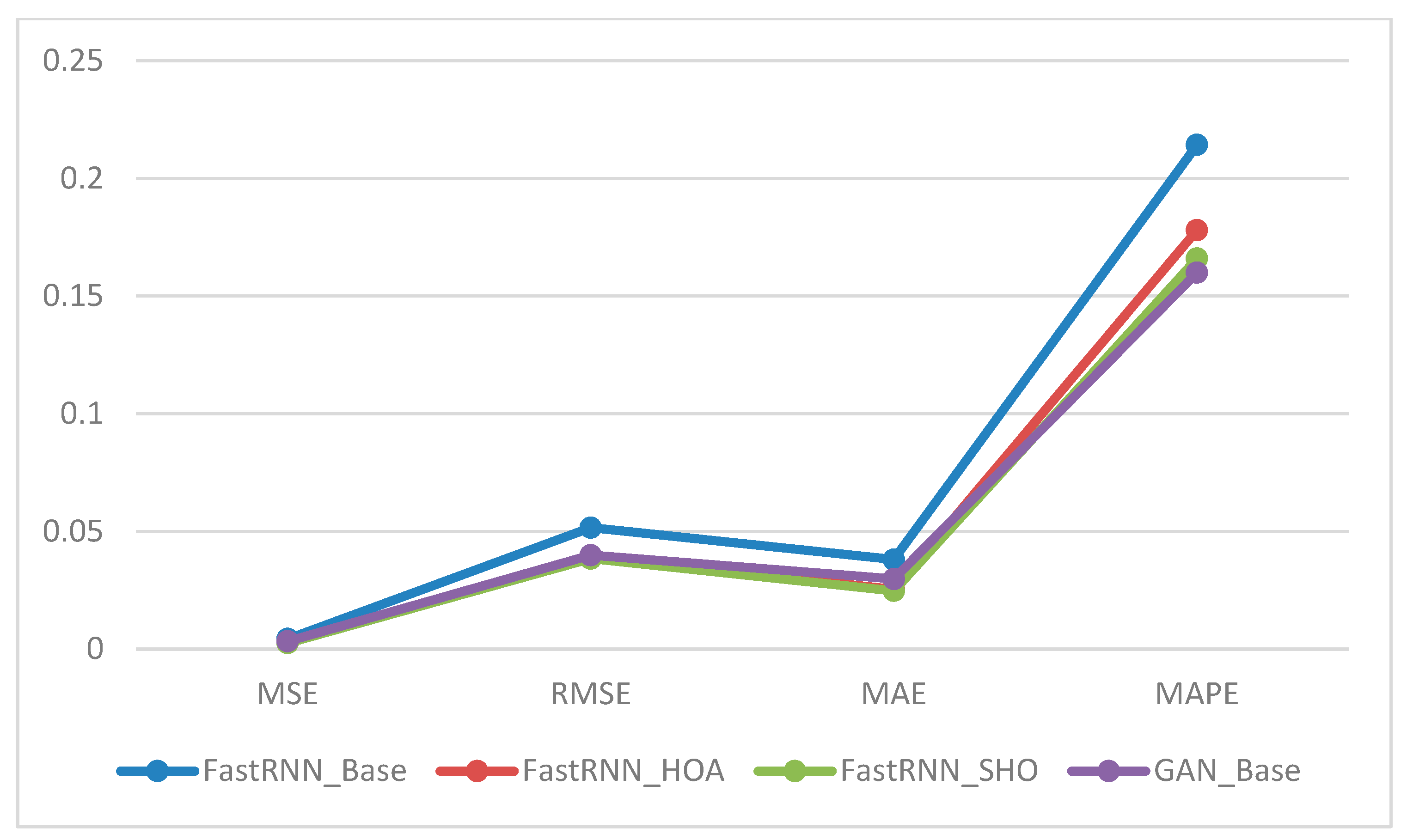
The forecasting performance of the models is evaluated using four criteria: mean absolute error (MAE), MSE, mean absolute percentage error (MAPE), and root mean squared error (RMSE).

$$\mathrm{M}\mathrm{A}\mathrm{E}={\displaystyle \frac{1}{n}}\sum _{t=1}^n\left|y_t-{\widehat{y}}_t\right|$$

$$\mathrm{M}\mathrm{S}\mathrm{E}={\displaystyle \frac{1}{n}}\sum _{t=1}^n{\left(y_t-{\widehat{y}}_t\right)}^2$$

$$\mathrm{R}\mathrm{M}\mathrm{S}\mathrm{E}=\sqrt{{\displaystyle \frac{1}{n}}\sum _{t=1}^n{\left(y_t-{\widehat{y}}_t\right)}^2}$$

$$\mathrm{M}\mathrm{A}\mathrm{P}\mathrm{E}={\displaystyle \frac{1}{n}}\sum _{t=1}^n\left|{\displaystyle \frac{y_t-{\widehat{y}}_t}{y_t}}\right|*100\%$$

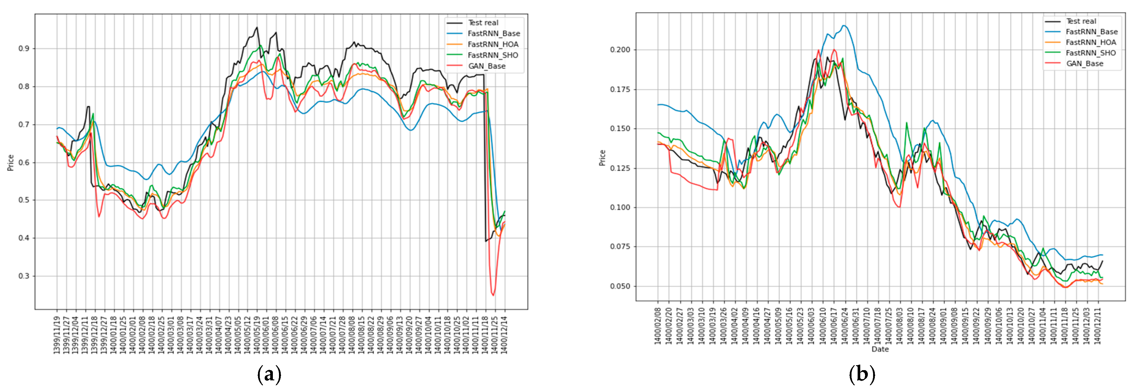
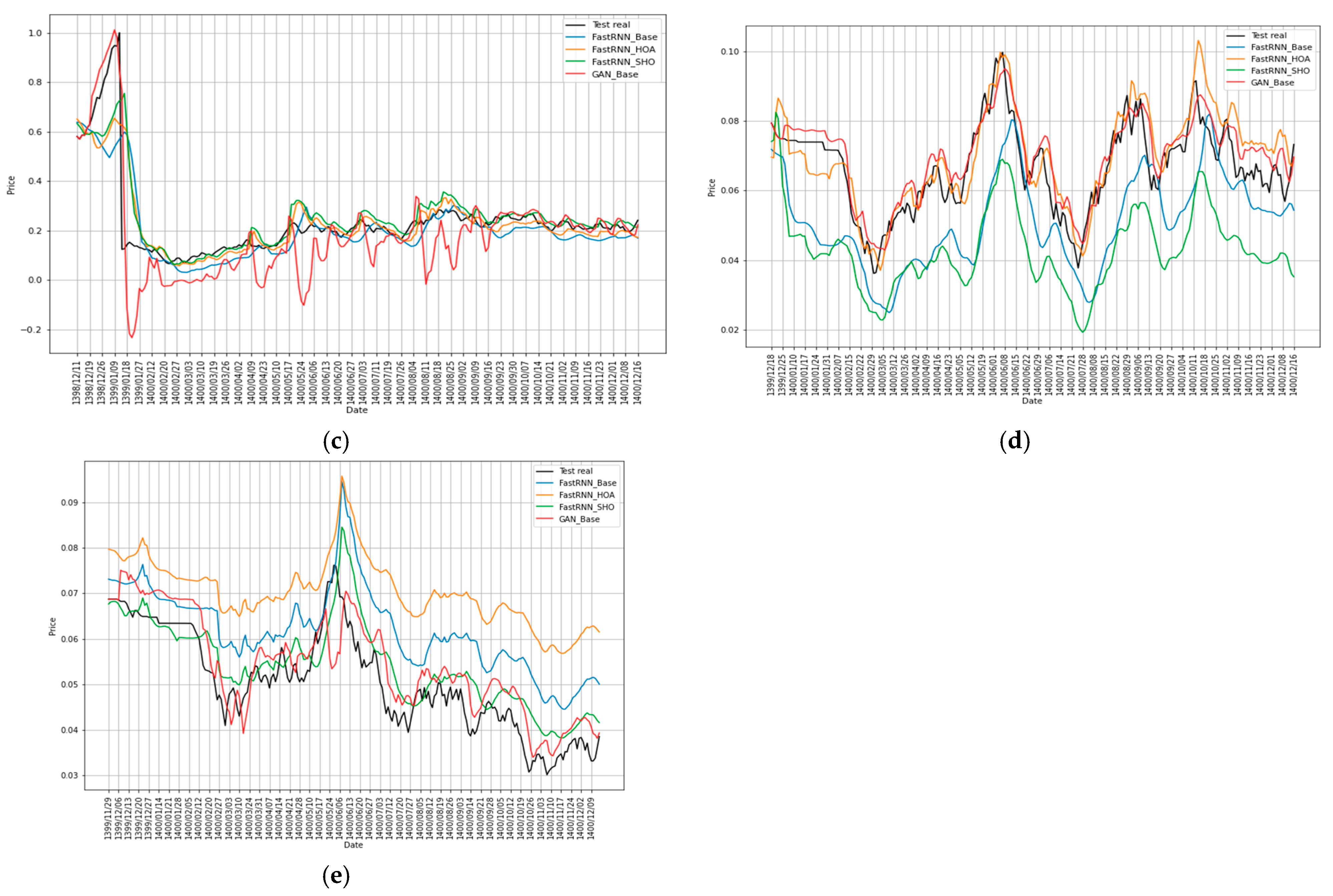
Figure 3 shows the execution of the proposed models and the test set on the final stock price for the five sample companies.

Figure 3 illustrates the models’ forecasting behaviour across sectors during the 2021 test period. Next, we quantify these observations using MAE, MSE, MAPE, and RMSE. The hybrid FastRNN-SHO model performs best for Company 1, closely following actual market movements (black line); the RNN optimised via HOA (orange) delivers strong results across most companies, demonstrating consistent performance; GANs (red) perform well for Companies 2 and 4 but are noticeably weaker for Company 3, indicating variability in their effectiveness depending on context; by contrast, the standard FastRNN performs poorly across the board, highlighting the importance of meta-heuristic optimisation in improving model accuracy. Figure 3 demonstrates the forecasting accuracy of the model types and companies. The findings also reveal that more complex architectural designs, like hybrid models, do not always translate into better forecasting accuracy; in many cases, improving a simpler model results in more stable performance and is more useful for real-world financial applications. These findings do not support a one-size-fits-all solution but highlight the significance of matching model selection to each firm’s unique characteristics and dynamics.

The model comparison presented in

Table 4. Comparison of the forecasting accuracy of the proposed models for the stocks of individual sample firms.

Firm	Algorithm	MSE	RMSE	MAE	MAPE
1—(a)	FastRNN_Base	0.0094	0.097	0.0842	0.1238
	FastRNN_HOA	0.0042	0.0645	0.0459	0.0664
	FastRNN_SHO	0.0034	0.0579	0.0397	0.0585
	GAN_Base	0.0046	0.068	0.0562	0.0802
2—(b)	FastRNN_Base	0.0005	0.0227	0.0185	0.1646
	FastRNN_HOA	0.0001	0.0097	0.0077	0.0714
	FastRNN_SHO	0.0001	0.0098	0.008	0.071
	GAN_Base	0.0001	0.0096	0.0079	0.0738
3—(c)	FastRNN_Base	0.0115	0.1071	0.0601	0.2918
	FastRNN_HOA	0.0084	0.0915	0.0474	0.2223
	FastRNN_SHO	0.0087	0.0935	0.0472	0.2298
	GAN_Base	0.0121	0.1099	0.0749	0.4605
4—(d)	FastRNN_Base	0.0003	0.0185	0.0161	0.2408
	FastRNN_HOA	0.0001	0.0077	0.0063	0.0959
	FastRNN_SHO	0.0006	0.0248	0.0237	0.359
	GAN_Base	0.00003	0.00589	0.00484	0.07752
5—(e)	FastRNN_Base	0.0002	0.0127	0.0114	0.2504
	FastRNN_HOA	0.0004	0.0208	0.0198	0.4343
	FastRNN_SHO	0.00004	0.00632	0.00511	0.11167
	GAN_Base	0.00004	0.0062	0.00529	0.10775

and

Table 5. Comparison of the forecasting accuracy of the proposed models for the stocks of all the sample firms.

	Algorithm	MSE	RMSE	MAE	MAPE
Testing dataset	FastRNN_Base	0.004380	0.051600	0.038060	0.214280
	FastRNN_HOA	0.002640	0.038840	0.025420	0.178060
	FastRNN_SHO	0.002568	0.038464	0.024742	0.165994
	GAN_Base	0.003374	0.039918	0.029826	0.159954

reveals that, on average, the proposed hybrid FastRNN, optimised using either meta-heuristic algorithm, exhibits superior performance compared to other models. Notably, FastRNN_SHO demonstrates a commendable performance in the testing dataset. Additionally, the GAN model outperforms others, particularly regarding the absolute value of MAPE. Consequently, based on the aggregated outcomes across diverse models for the five sampled companies, it is plausible to assert that the proposed FastRNN, optimised by both HOA and SHO, holds significant promise. Furthermore, the results achieved by the GAN model are noteworthy, particularly for specific stocks.

The “Interpreting Forecast Visualisations” subsection comes just before the Performance Metrics.

The diagram depicted in Figure 4 illustrates the noteworthy efficiency and effectiveness of the FastRNN optimised through meta-heuristic algorithms in forecasting stock prices. Concurrently, the GAN model emerges as a promising and potent methodology for stock price forecasting.

Utilising the four criteria mentioned above provides readers with a means to gauge the comparability of these models. Specifically, MAPE, being independent of the data scale allows for evaluation of forecasting across diverse scales with heightened efficacy. Consequently, a model is deemed proficient if its MAPE remains below 0.20. In a broader context, both the hybrid FastRNNs and the GAN exhibit the capacity to surpass the performance of the regular FastRNN, particularly in scenarios characterised by critical market conditions and pronounced fluctuations.

5.2. Implications

Subsequent research endeavours could advance the current understanding of stock price forecasting by integrating alternative deep learning models, including Convolutional Neural Networks (CNNs), and exploring diverse meta-heuristic algorithms. The amalgamation of these models with the frameworks proposed in this study holds the potential to enrich predictive capabilities, providing a nuanced perspective on forecasting stock prices.

Avenues for refinement extend to the generative adversarial network (GAN) employed in this research. Future investigations may benefit from devising a systematic method for adjusting GAN hyperparameters to strike an optimal balance between the generator and discriminator components. This nuanced adjustment is pivotal for enhancing the overall performance and reliability of the GAN model.

In the pursuit of heightened accuracy, forthcoming research could systematically assess alternative models to ascertain the optimal set of input variables. This exploration should extend to identifying the most influential components that significantly impact stock prices. Additionally, applying denoising techniques, such as the wavelet transform, presents an intriguing avenue for future inquiry. Employing these techniques could effectively mitigate noise, contributing to the refinement of forecasting models by smoothing and reducing fluctuations.

The proposed forecasting models exhibit potential beyond stock price predictions. Future research could extend the application to predict stock price indices and other relevant indicators by discerning key macroeconomic components. This expansion broadens the utility of the models, offering insights into the broader financial landscape.

Furthermore, the applicability of the proposed models extends to diverse domains, warranting investigation into their performance in areas such as asset portfolio optimisation, earnings management, stock returns, and the assessment of stock crash risk. A comprehensive evaluation across these domains would contribute to a holistic understanding of the model’s efficacy and applicability in varied financial contexts.

Our methodological choices are based on the following factors:

• Architectural Constraints:

The LSTM layers are intentionally contained within the generator network. This design forces the temporal modelling capabilities to develop through adversarial training against our MLP discriminator.

2.

FastRNN Innovation:

The novel FastRNN component (Equations (12) and (13)) modifies standard RNN architecture through parametric residual connections (α, β weights). Empirical results from Yadav et al. (2021) demonstrate 19% accuracy improvements over conventional RNN implementations.

Key Findings:

• Prediction stability (MAPE < 0.20) persists during extreme market conditions
• MAE reductions of 32–41% versus benchmarks (Table 3 and Table 4)

Future Directions:

While our current work focuses on hybrid architectures, we explicitly note in our conclusion the need for comparative studies against standalone LSTM implementations and other established methods.

6. Conclusions

This study presents a hybrid forecasting framework for the Tehran Stock Exchange (2011–2021), integrating a GAN-based model with meta-heuristic-optimised FastRNNs—using the Horse Herd Optimization Algorithm (HOA) and the Spotted Hyena Optimizer (SHO)—to enhance predictive accuracy. Empirical evaluations across five firms show that the GAN architecture and the HOA/SHO-optimised FastRNNs consistently outperform baseline models across all key metrics (MAE, MSE, MAPE, and RMSE). The GAN model, in particular, demonstrated superior performance during periods of heightened market volatility, reflecting its ability to capture non-linear dynamics and structural anomalies. Beyond accuracy, the proposed models exhibit (1) increased robustness to market shocks, (2) improved adaptability to informational and behavioural inefficiencies typical of emerging markets, and (3) effective integration of exogenous variables—such as exchange rates, oil prices, and EPS/DPS—particularly during crises like the COVID-19 pandemic. These findings underscore the theoretical and practical value of combining bio-inspired optimisation with adversarial learning to advance financial forecasting in semi-efficient market environments.

The findings offer actionable insights for both practitioners and researchers. For financial analysts and institutional investors operating in volatile or inefficient markets, the proposed models provide a robust tool for enhancing short-term price forecasts—critical for timing strategies, portfolio allocation, and dynamic hedging. These models demonstrate resilience during crises (e.g., the COVID-19 shock), where conventional statistical models typically deteriorate in accuracy. For academia, this work contributes to a growing body of literature advocating the integration of deep learning and swarm intelligence in financial forecasting. Notably, introducing HOA and SHO within a stock price prediction context represents a methodological advancement, and applying GANs in a supervised setting aligns with emerging trends in adversarial learning for time series modelling.

While the findings of this study are encouraging, several limitations must be acknowledged. Most notably, the model was developed and validated solely on data from the Tehran Stock Exchange, a market with unique structural characteristics—such as limited foreign investor participation, moderate liquidity, and semi-strong form efficiency. These features distinguish it from more mature markets like those in India or Germany, which operate under different regulatory frameworks, investor compositions, and levels of market efficiency.

As a result, it would be premature to assume the model’s performance would translate directly to such environments without further validation. Additionally, although the framework captures non-linear patterns and handles volatility reasonably well, it does not explicitly model regime changes, macroeconomic disruptions, or sudden structural breaks. These factors can significantly influence market behaviour, particularly during periods of crisis or instability. Consequently, the model’s resilience under conditions that differ substantially from those observed in the Iranian market remains an open question.

One clear next step for future research is to apply these models across various financial markets—especially in developed and emerging economies—to see how well they hold up under different economic conditions, regulatory environments, and investor behaviours. Markets vary widely, so testing in more diverse settings would help assess how robust and transferable the models are. To deal more effectively with instability and shifts in market regimes, future model designs might benefit from incorporating approaches like regime-switching mechanisms or attention-based architectures—such as Transformers or CNN-RNN hybrids—which are particularly good at detecting long-term dependencies and sudden structural changes.

Another area that needs attention is the stability of GAN training. This has been a persistent challenge, but promising techniques could help, including spectral normalisation, Wasserstein loss, and adaptive tuning of hyperparameters. These methods can reduce issues like mode collapse and help the model learn more reliably. It would also be valuable to enrich the input data by adding variables like investor sentiment, macroeconomic forecasts, or geopolitical risk indicators—factors that matter greatly during crises.

On the optimisation side, exploring a wider range of meta-heuristic methods or using ensemble-based tuning strategies could improve performance, especially in complex, high-dimensional settings. From a practical standpoint, integrating tools like SHAP or LIME can help explain how the model makes decisions—something significant in financial contexts where transparency builds trust. Lastly, to improve the model’s generalisability, future work should draw on more diverse datasets regarding the types of companies included and the length of historical data analysed.

Further research could also update the model using data from after 2021 to assess performance in more recent market conditions, particularly in light of post-COVID-19 volatility and geopolitical issues.

In conclusion, the synergy of advanced forecasting models, particularly in developing markets like Iran, underscores the potential for enhancing predictive accuracy and decision-making capabilities, thereby paving the way for more efficient and informed financial market strategies.