Article

The Effect of Different Saving Mechanisms in Pension Saving Behavior: Evidence from a Life-Cycle Experiment

1
Liechtenstein Business School, University of Liechtenstein, Fürst-Franz-Josef-Strasse, 9490 Vaduz, Liechtenstein
2
Newcastle Business School, Northumbria University, Newcastle upon Tyne NE1 8ST, UK
3
Halle Institute for Economic Research, 06108 Halle (Saale), Germany
*
Author to whom correspondence should be addressed.
J. Risk Financial Manag. 2025, 18(5), 240; https://doi.org/10.3390/jrfm18050240
Submission received: 27 February 2025 / Revised: 29 March 2025 / Accepted: 11 April 2025 / Published: 1 May 2025
(This article belongs to the Special Issue Pensions and Retirement Planning)

Abstract

:
We examine how institutional saving mechanisms influence retirement saving decisions under bounded rationality and income risk. Using a life-cycle experiment with habit formation and loss aversion, we test mandatory and voluntary binding savings under deterministic and stochastic income. Voluntary commitment improves saving performance only when income is predictable; under uncertainty, it fails to improve performance. Mandatory savings do not raise total saving, as participants reduce voluntary contributions. These results emphasize the role of income smoothing in enabling behavioral interventions to improve long-term financial outcomes.
JEL Classification:
C90; D91; H55

1. Introduction

Why do individuals often fail to save adequately for retirement, despite understanding its long-term importance? Canonical economic models assume that people behave as rational planners, dynamically allocating income to smooth consumption over their lifetime (Friedman, 1957; Modigliani & Brumberg, 1954). However, the growing literature shows that individuals systematically deviate from these predictions (Benartzi & Thaler, 2013; Lusardi, 1999; Thaler, 1994). Experimental studies find that even under idealized conditions, individuals often fail to solve dynamic consumption-saving problems optimally (A. L. Brown et al., 2009; Duffy & Orland, 2023; Fenig & Petersen, 2024). Recent experimental evidence reinforces these concerns (Duffy & Orland, 2023; Fenig & Petersen, 2024). These behavioral shortcomings raise important policy questions for pension system design. If saving behavior is systematically suboptimal, what institutional mechanisms can help individuals make better decisions? Should pension systems rely on mandatory contributions, or can voluntary commitment devices enhance outcomes—particularly under income uncertainty, where planning is more difficult?
This paper evaluates the effects of two commonly used mechanisms in pension systems: (i) obligatory savings and (ii) a combination of obligatory and voluntary binding savings. Using a life-cycle experiment, we test how these mechanisms affect individual utility in environments with deterministic and stochastic income. Our goal is to assess whether such mechanisms improve outcomes for participants with bounded cognitive abilities and whether their efficacy depends on income predictability. In a series of laboratory experiments, we examine how different saving mechanisms affect a person’s ability to maximize utility from intertemporal consumption-saving decisions. The decision environment is structured into two phases: a working life (income-generating periods) and a retirement phase (periods with no income). Participants earn utility by “consuming” portions of their income, guided by an induced utility function that incorporates two key behavioral features: loss aversion and habit formation. To investigate the influence of saving mechanisms, we implement a 2 × 3 between-participant design, where we vary the nature of the income stream (deterministic or stochastic), as well as the saving mechanisms available to participants. Here, we differentiate three conditions: (i) Baseline: Participants manage a single account for all savings (“pocket savings”), accessible throughout the experiment. (ii) Obligatory Retirement Contributions: Participants make mandatory payments into a retirement account during their working life, which can only be accessed during the retirement phase, similar to defined contribution pension plans. (iii) Voluntary Binding Savings: Alongside obligatory contributions, participants can set aside additional savings into a third account designated for retirement. These settings allow us to observe how different saving mechanisms affect consumption behavior and utility maximization over time.
Our paper makes three contributions to the literature on savings behavior and pension system design. First, we propose an experimentally implementable formulation of intertemporal utility that incorporates empirically supported features of human preferences—namely, loss aversion and habit formation—while remaining simple and intuitive enough for experimental participants to engage with meaningfully. Second, we experimentally evaluate two savings mechanisms widely used in European pension systems: mandatory contributions and a combination of mandatory and voluntary binding savings. Unlike many prior studies that impose structural constraints on consumption decisions, our design allows participants full flexibility to consume or save their income at any point during the working or retirement stages of the life cycle. This enables us to examine both the demand for institutional saving mechanisms and their behavioral effects on consumption smoothing and welfare outcomes. Our design also reflects recent calls to test the efficacy of such mechanisms in environments where individuals face planning constraints or cognitive limitations (e.g., Bachmann et al., 2023). Third, we contribute to the literature on precautionary saving and behavioral responses to uncertainty by comparing decision making under deterministic and stochastic income. While prior work has shown that income volatility interacts with liquidity constraints and cognitive skills to shape saving behavior, few studies have examined whether the same institutional mechanisms are effective across these environments. By holding preferences and institutional structure constant across income regimes, our experiment isolates the behavioral consequences of income uncertainty and tests the robustness of institutional designs.
Our results replicate key findings from previous life-cycle experiments, including the characteristic hump-shaped pattern of overconsumption/undersaving during the working life and positive effects of learning on saving performance over time. When comparing participants exposed to deterministic vs. stochastic income streams, we find that individuals facing income uncertainty consistently underperform relative to their counterparts with stable income. Notably, voluntary commitment devices—despite their promise as behavioral tools to counteract undersaving—fail to improve outcomes under stochastic income conditions. These findings underscore the importance of income predictability as a prerequisite for the effectiveness of behavioral interventions and suggest that income smoothing may be a necessary complement to commitment-based instruments in the design of modern pension systems.
The paper is organized as follows: Section 2 discusses the relevant literature that inspires the hypotheses in Section 3. Section 4 describes the experimental design. Section 5 presents our results, and Section 6 concludes.

2. Background Literature

2.1. Retirement Planning and Bounded Rationality

The standard literature on household retirement saving builds on the assumption that individuals act as rational planners, allocating their income between consumption and saving to maximize lifetime utility, as proposed in the “life-cycle hypothesis” (Modigliani & Brumberg, 1954). According to this model, individuals aim to smooth consumption over time by saving during high-income periods and dissaving during retirement (Friedman, 1957). However, a growing body of behavioral and experimental research shows that individuals often deviate from these predictions, systematically under-saving for retirement and responding to features of the decision environment that should be irrelevant under full rationality (Benartzi & Thaler, 2013).
While many standard saving experiments focus on one-shot or short-horizon decisions—often isolating particular mechanisms or incentives—life-cycle experiments require individuals to solve dynamic optimization problems across multiple periods, typically involving planning under constraints, uncertainty, and feedback. These tasks impose higher cognitive demands and more closely reflect the structure of real-world retirement planning. Importantly, life-cycle experiments allow researchers to compare observed behavior against normative benchmarks derived from backward induction, making them well suited for assessing the degree and structure of suboptimality in saving behavior.
Existing life-cycle experiments consistently show that individuals tend to overconsume early in life and fail to accumulate sufficient retirement savings, even when such plans are feasible and optimal (Duffy & Li, 2019). These deviations are often attributed to limited cognitive ability, myopic preferences, and difficulties in planning across multiple stages of life (Ballinger et al., 2011; Harris & Laibson, 2001; Lusardi, 1999). Recent studies reinforce this view; Fenig and Petersen (2024) and Duffy and Orland (2023) find persistent departures from theoretical optima even in deterministic environments with full information.
In an extensive replication study, Bachmann et al. (2023) confirm that life-cycle decisions remain suboptimal even in simplified task designs adapted for broader populations. These findings support the view that bounded rationality is a key constraint in retirement saving and must be explicitly addressed in policy and experimental design.

2.2. Saving Decisions in Different Environments

Experimental evidence shows that institutional design plays a central role in shaping retirement saving behavior, particularly when individuals face cognitive or informational constraints. Commitment devices—such as restricted-access accounts or early withdrawal penalties—have been shown to increase savings by helping individuals overcome self-control problems (Ashraf et al., 2006; Beshears et al., 2015a, 2020). However, their effectiveness depends on how they are embedded in broader institutional settings and how they interact with individual preferences and planning ability.
A related line of research focuses on the role of framing and default rules in retirement decision making. Experimental studies demonstrate that annuitization, asset allocation, and retirement timing decisions are highly sensitive to how options are presented. Framing effects can lead to substantial deviations from normative benchmarks even when underlying incentives remain constant (Agnew et al., 2008, 2015; J. R. Brown et al., 2008). Davidoff et al. (2005) show that relatively small institutional frictions can account for low annuity take-up, challenging the explanatory power of standard models. Fatás et al. (2013) and Card and Ransom (2011) likewise find that the form of benefit payments and default structures can meaningfully alter behavior.
Bachmann et al. (2023) replicate several of these institutional effects using larger and more diverse samples. They confirm that matching contributions are more effective than tax rebates and that annuity framing influences retirement timing. However, they also document that increased task complexity and ambiguity can substantially dampen responsiveness to institutional incentives, particularly when cognitive demands are high. This highlights the importance of designing interventions that are both behaviorally effective and cognitively accessible.

2.3. Saving Decisions Under Stochastic Income

The empirical relevance of precautionary saving under income uncertainty remains contested. Standard theory predicts that income risk should lead to higher savings (Gourinchas & Parker, 2002; Zeldes, 1989), but the experimental results are mixed. Some studies find support for increased saving in the presence of volatility (Carbone & Hey, 2004), while others do not (Meissner, 2016). Cognitive constraints may partly explain this inconsistency. The recent work confirms that income unpredictability reduces the effectiveness of saving mechanisms. Duffy and Orland (2023) show that while participants respond directionally to shocks, their behavior remains systematically off the theoretical benchmark. Kappes et al. (2023) find that scarcity and income predictability interact to determine consumption smoothing success.
Our study contributes to this literature by testing how voluntary and mandatory saving mechanisms perform under deterministic vs. stochastic income profiles in a controlled life-cycle experiment. In contrast to previous studies that typically examine income uncertainty or institutional mechanisms in isolation, our study combines both dimensions in a unified life-cycle experiment with an induced behavioral utility function. This design allows us to evaluate whether mechanisms that are effective under certainty retain their efficacy under income risk, thereby providing new evidence on the interaction between institutional design and bounded rationality in retirement saving behavior.

3. Hypotheses

Drawing on the literature reviewed in Section 2, we derive the following hypotheses, focusing on typical deviations from optimal saving behavior, the role of income uncertainty, and the impact of institutional mechanisms.

3.1. Hypothesis I: Undersaving/Overconsumption

A wide range of empirical and experimental studies reports consistent undersaving, often attributed to bounded rationality, cognitive constraints, or behavioral biases. Repetition has been found to mitigate such effects by allowing participants to learn (for a review, see Duffy, 2008). We therefore expect that (i) retirement savings will initially be lower than optimal and (ii) this behavior improves with repeated exposure to the task.
H Ia:
Participants achieve less than optimal utility due to inadequate retirement savings.
H Ib:
Repeating the task leads to higher utility due to reduced undersaving/overconsumption.

3.2. Hypothesis II: Income Uncertainty

Income uncertainty can influence saving behavior in opposing ways. Theoretically, risk should lead to increased precautionary saving (Gourinchas & Parker, 2002; Skinner, 1988; Zeldes, 1989), which may help reduce overconsumption and raise utility. Conversely, if individuals tend to undersave, then due to loss aversion, negative income shocks could lower utility more than positive ones improve it. We therefore propose two competing hypotheses:
H IIa:
Participants earn higher utility under stochastic income conditions due to increased precautionary savings.
H IIb:
Participants earn lower utility under stochastic income conditions due to the negative effects of income shocks outweighing any positive effects.

3.3. Hypothesis III: Savings Mechanisms

Many European pension systems rely on obligatory contributions to reduce undersaving (Hinrichs, 2021), but it remains debated whether such mechanisms increase total savings or simply displace voluntary ones (Duffy & Li, 2019). Moreover, their impact on life-cycle utility is unclear. This leads to the following hypothesis:
H IIIa:
Participants earn higher utility in the presence of an obligatory contribution mechanism than in its absence.
In contrast, commitment devices and awareness-enhancing interventions have shown promise in supporting self-control and improving saving outcomes (Karlan et al., 2016; Rha et al., 2006; Rodríguez & Saavedra, 2015). Voluntary but binding mechanisms combine both elements. Their use in real-world pension systems—alongside mandatory contributions—has been expanding (Ebbinghaus, 2021; Rudolph, 2016). We therefore state the following:
H IIIb:
Participants earn higher utility when a voluntary but binding saving mechanism is available, as it will reduce undersaving compared to settings with only mandatory or non-binding voluntary contributions.

4. Experimental Design

4.1. The Consumption-Saving Task

Our experimental design builds on the standard life-cycle consumption framework (Modigliani & Brumberg, 1954), where participants optimize the sum of immediate and future consumption utility based on expected lifetime income. All participants live for T periods.1 In each period, they earn utility by consuming part of their income. Since we are interested in an individual’s ability to sustain themselves during retirement, we divide the individual’s lifetime into working periods (t = 1, …, τ ) and retirement periods (t = τ + 1, …, T), with consumption during retirement financed by prior savings. While working, the individual receives labor income y t in each period, which can be used for immediate consumption or saved for consumption in later periods. No labor income is earned during retirement when all consumption has to be financed by savings from previous periods. Participants cannot consume more than their current actual income plus prior savings. Borrowing is excluded to simplify the task. For the same reason, the savings rate is set to zero, following, e.g., Ballinger et al. (2011, 2003); Feltovich and Ejebu (2014); Gechert and Siebert (2022). The optimization problem is expressed as
max c t E t = 1 T u t s . t . s t = y t + s t 1 c t t [ 1 , τ ] ,   s 0 = 0 s t = s t 1 c t t [ τ + 1 , T ] ,   s T = 0
Here, s t represents savings, y t is income, and u t is the utility in period t.

4.1.1. Consumption Utility

While individual preferences may vary, controlled experiments allow us to induce a uniform consumption utility structure, enabling the derivation of optimal consumption paths despite the heterogeneity of actual individual preferences (Hey & Dardanoni, 1988). Using an induced utility function is an established and essential practice in experimental economics (see Bachmann et al. (2023) for a replication survey.), as it ensures a controlled environment where participants’ consumption choices can be analyzed. The induced utility structure reflects average consumer behavior derived from prior experimental and empirical research (e.g., Carroll et al., 2000; Fehr & Zych, 1998). This approach is necessary because we lack detailed knowledge of each participant’s unique utility function. By employing the parameters validated in previous studies, we create a standardized model that captures realistic decision-making patterns while allowing comparisons between participants’ observed and optimal behavior. Implementing an induced utility function also motivates participants to distribute their consumption over time, which is critical in experiments without interest on savings or periodic payoffs (Bachmann et al., 2023). Without such a structure, participants may concentrate their consumption in select periods, diminishing the realism of the data generated. Furthermore, this design maintains external validity by retaining common, influential features in real-world decision making, such as (i) loss aversion and (ii) habit formation, which complicate consumption–saving decisions in practice. To simplify participant engagement and avoid framing effects tied to economic terminology, we refer to the induced utility function as “points” rather than explicitly using the term “utility”. This wording encourages participants to focus on strategic decisions related to saving and consumption within the experiment, thereby aligning their decisions with intuitive behavioral responses rather than economic concepts.

4.1.2. Loss Aversion

Loss aversion in our setting refers to the heightened sensitivity of individuals to consumption falling below the current habit level. To model loss aversion, we build on the utility function proposed by Bowman et al. (1999):
u t ( h t , c t ) = α × h t y ¯ + c t h t y ¯ α , c t > h t , α × h t y ¯ β × h t c t y ¯ α , c t h t ,
where c t is the level of consumption, and h t is the consumption habit in period t. α and β are parameters for risk aversion and loss aversion, respectively.
This formulation is a variation of the value function introduced in prospect theory (Tversky & Kahneman, 1992). Based on a comprehensive review of empirical evidence on parameter values (Camerer & Ho, 1994; Tversky & Fox, 1995; Wu & Gonzalez, 1996), we select α = 0.85 and β = 2 , which are widely supported across studies.

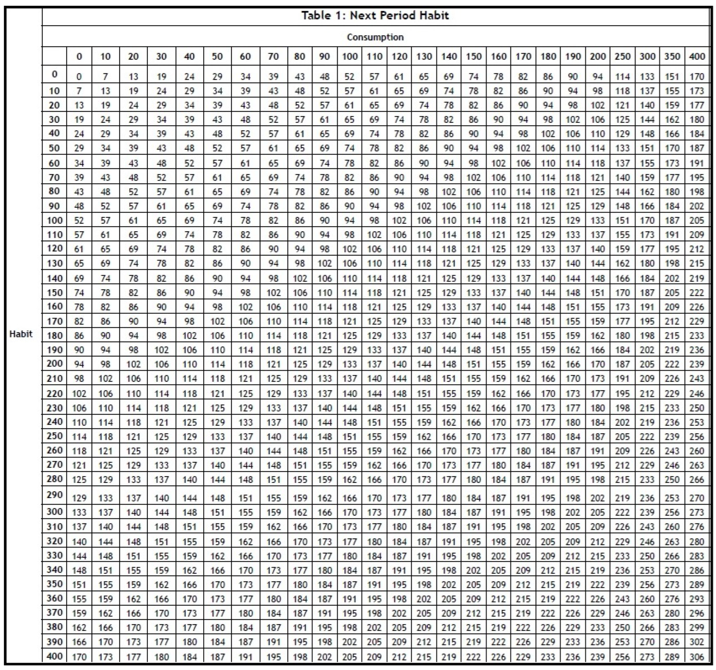
4.1.3. Habit Formation

In dynamic consumption-saving decisions, habits form endogenously based on past consumption. Empirical studies show that consumption utility depends on both current and past consumption (Carroll et al., 2000; Fuhrer & Klein, 1998; Marshall, 2005). Moreover, habit growth slows asymptotically (Lally et al., 2010). To capture this, we modify the habit formation model of Carroll (2000) to incorporate diminishing habit growth:2
h t = y ¯ × λ × h t 1 + ( 1 λ ) × c t 1 y ¯ ϕ ,
where c t and h t denote the levels of consumption and habit at time t, and λ and ϕ are parameters. We choose ϕ = 0.85, which implies moderate concavity.3 Again, we divide by y ¯ to impose homogeneity, yielding relative values for consumption and habit.

4.2. Treatment Conditions

4.2.1. Baseline

In our baseline setting, one life cycle consists of fifteen consecutive consumption-saving decisions, where the first ten periods represent the working life and the last five constitute retirement. Using this setting, we implement a 2 × 3 experimental design where (i) participant income during the working life is either deterministic or stochastic, and (ii) participants have the choice among different saving mechanisms.

4.2.2. Deterministic vs. Stochastic Income

We implement two variants of participants’ working income, y t : (i) deterministic income and (ii) stochastic income. In treatments with deterministic income (Det), participants receive 100 experimental currency units (ECU) in each of the first ten periods. This is commonly known. In treatments with stochastic income (Stoch), the per-period income is randomly drawn from the set { 80 , 100 , 120 } with equal probabilities. The random draws in each period are independent of the draws in any other period. This income structure was completely revealed to the participants during the introduction of the experiment and therefore common knowledge. To control for path dependence but still keep observations comparable, we randomly generate two income paths (Path 1 and Path 2) before conducting the experiment. Half of the participants in stochastic income treatments faced Path I in their first and Path II in their second life cycle, and vice versa for the other half. This procedure is important to allow for the calculation of optimal behavior conditional on the actual realization of the income stream.
Using the life-cycle model outlined above, we calculate the optimal saving and consumption paths, which serve as a benchmark for evaluating the participants’ decision making. We solve the optimization problem in equation (1) using backwards induction, allowing us to derive consumption paths under both deterministic and stochastic income conditions. This benchmark helps assess how closely the participants’ behavior aligns with optimal decision making in the presence of behavioral constraints.
Figure 1 illustrates the optimal absolute consumption paths for both deterministic and stochastic income conditions (for more information on differences between the two stochastic paths, please check Table A1 in Appendix C). Despite minor differences, the optimal paths for both stochastic income scenarios remain relatively close to the deterministic path, indicating that uncertainty has limited effects on the theoretical benchmark for consumption.
For the given income paths, the optimal saving and consumption decisions are feasible throughout the experiment. Importantly, optimal savings exceed obligatory contributions, suggesting that from a rational planner perspective, neither mandatory nor voluntary saving mechanisms bind the participants’ choices. Consequently, any deviations from optimality observed in the experiment can be attributed to behavioral factors, such as loss aversion or habit formation, rather than institutional constraints.

4.2.3. Saving Mechanisms

Pension systems vary widely, particularly in the types of available saving mechanisms and the level of access to funds prior to retirement.4 However, many European systems share common features, including mandatory contributions to a pension account and the option of a voluntary savings account dedicated to retirement savings (Hinrichs, 2021). Our experiment aims to analyze these core elements in a simplified way (e.g., neglecting tax rules).
To do so, we implement three distinct institutional environments, each offering the participants different saving mechanisms. We summarize them in Table 1 In each case, savings s t can be accumulated through one or a combination of the following mechanisms: pocket savings, obligatory savings and voluntary savings. To distinguish these combinations while avoiding any confusion with real-world pension systems, we will call them settings 1–3.
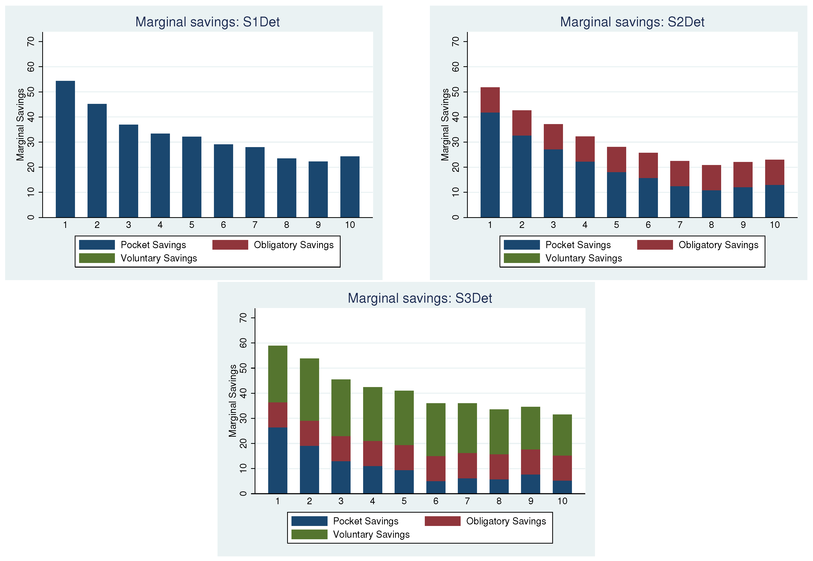
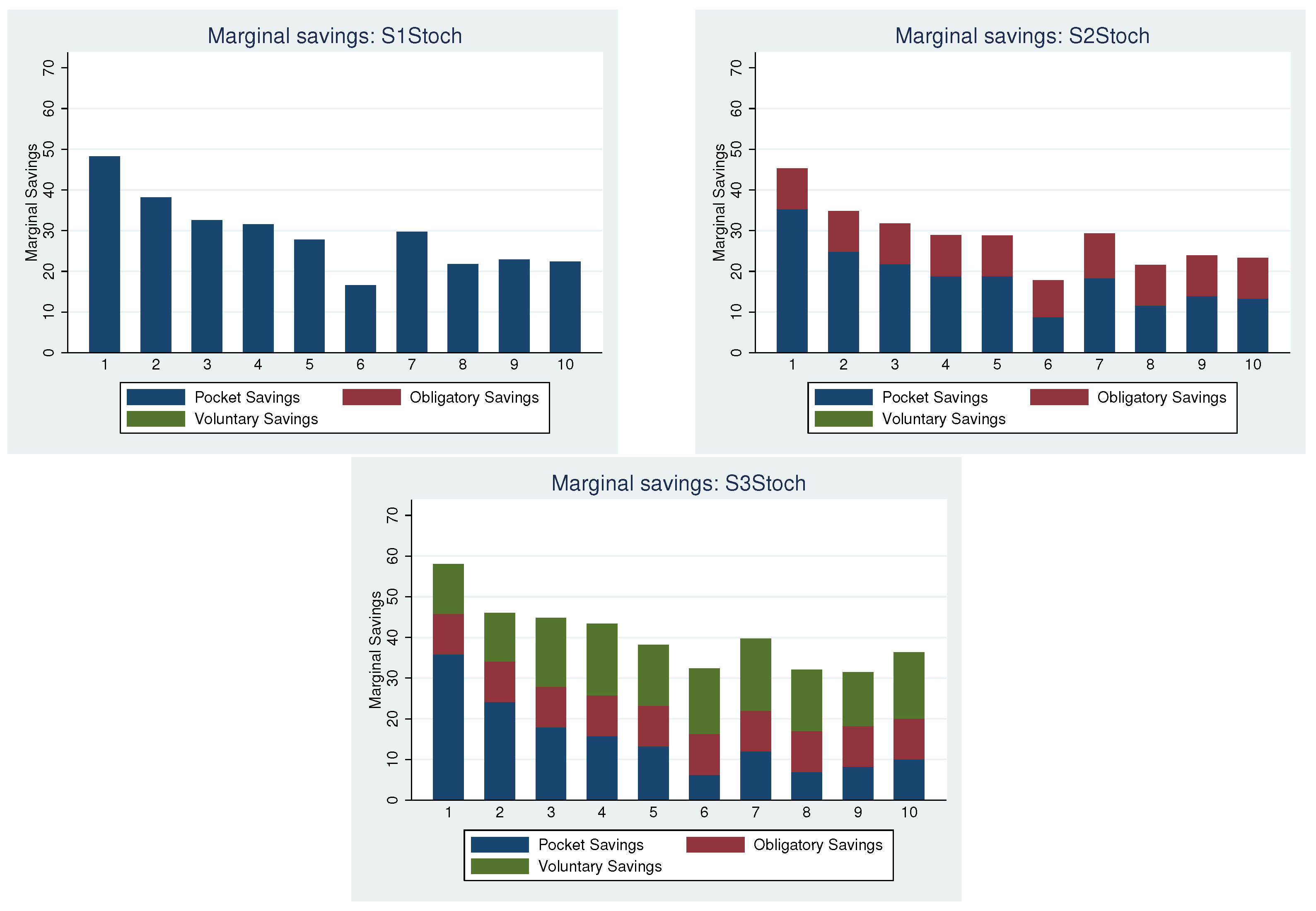
  • Setting 1 (S1): All unspent income automatically becomes pocket savings ( p s t ), which can be accessed at any time. Total retirement savings t = 1 τ s t equal p s τ .
  • Setting 2 (S2): Participants must contribute 10% of their work life income each period to an obligatory pension savings account ( o s t ), which cannot be accessed until retirement starts in Period 11. During the working phase, obligatory savings increase by 0.1 × y t per period. Participants can still accumulate pocket savings by spending less than their disposable income, i.e., up to 0.9 × y t per period. At retirement, total savings s τ are the sum of pocket and obligatory savings: t = 1 τ s t = p s τ + t = 1 τ 0.1 y t .
  • Setting 3 (S3): In addition to the obligatory and pocket saving mechanisms from S2, participants can also make voluntary pension savings ( v s t ). Like obligatory savings, voluntary savings cannot be accessed before retirement. There is no interest advantage for holding funds in obligatory or voluntary accounts compared to pocket savings. Hence, total retirement savings are the sum of all three accounts: t = 1 τ s t = p s τ + t = 1 τ 0.1 y t + t = 1 τ v s t .

4.3. Implementation

The experiment was programmed in oTree (Chen et al., 2016) and conducted at the WiSo Experimental Laboratory in Hamburg. We ran six sessions with a total of 180 student participants. Participants spent approximately 60 min in the laboratory. Each treatment consisted of five parts: (1) questions to test cognitive abilities; (2) the BRET task; (3) questions to control for understanding of the main experiment (one treatment); (4) two life cycles of this treatment; (5) a demographic questionnaire.
The cognitive abilities of the participants were measured using the memory span task proposed by Conway et al. (2005). Before running the main part of the experiment, we asked participants multiple-choice questions to see whether they understood the main features of the experiment (the habit formation process, the utility function, etc.). If participants answered incorrectly, they were given a warning to rethink their answers. After finishing the life-cycle decision task, participants went through a short questionnaire asking for information about their age, gender and educational background. After the experiment, participants were paid for their participation, receiving an average payment of 11 EUR (see Appendix B for detailed information).
To reduce the computational burden on participants, we provided them with a table displaying various combinations of habit and consumption along with the corresponding utility values. Additionally, at the decision stage, a calculator was available to compute utility based on the participants’ chosen input values. Before starting the experiment, we ensured that all participants fully understood the task through comprehension checks. Since the utility function is complex and decreases sharply when choices deviate from the optimum, participants who failed to grasp the task would experience significantly lower utility. After identifying outliers, we excluded five participants (out of 180) who clearly did not understand the task, resulting in 175 fully independent observations for our analysis. The sample size—approximately 30 individuals per treatment cell—conforms to conventions in similar laboratory-based life-cycle experiments (for a review, see Bachmann et al., 2023) and provides adequate statistical power to detect medium-sized treatment effects in a between-participants design (Cohen, 1988).
The external validity of student samples has been examined in several studies. While students may differ from general populations in baseline behavior, their relative treatment responses are often consistent with those of non-students. For example, Cleave et al. (2013) show that selection effects exist but do not substantially distort treatment effects. Fréchette (2015) similarly finds that students and professionals respond comparably to experimental manipulations, even when their absolute behavior differs.
Falk and Heckman (2009) argue that the primary value of laboratory experiments lies in identifying behavioral mechanisms, not in generating population-level estimates, and that student samples are appropriate for this purpose. This rationale is particularly relevant in our context, as life-cycle consumption–savings models presuppose substantial cognitive capacities for solving dynamic optimization problems. Student samples may thus provide a conservative test of behavioral biases under bounded rationality, since participants are arguably better equipped to understand and engage with abstract intertemporal decision tasks. In that sense, the experimental design offers a favorable benchmark for evaluating deviations from rational behavior.

5. Results

5.1. Sample Characteristics

Table 2 summarizes descriptive statistics for our sample. There were more female than male participants, aged mostly between 20 and 30 years, and the vast majority of them hold a Bachelor’s or a Master’s degree. The background check reveals that only 2% of participants had already taken a course on pension decisions, whereas almost 90% did not have any prior specific knowledge in pension finance. A majority of participants (82%) successfully demonstrated their understanding of the experimental task at the first try in a quiz. Furthermore, most of the participants showed high cognitive abilities: 86% answered more than half of the logical questions correctly. We checked whether the distribution of these characteristics varies across treatments. Based on the results of a Chi-squared test, we found no significant differences across treatments with regards to gender, education, cognitive abilities, age of participants or their understanding of the experimental task (see Table 2).

5.2. Hypotheses Ia and Ib: Undersaving/Overconsumption

Figure 2 shows the average levels of consumption in each period across settings and life cycles together with the corresponding optimal consumption paths.5 On aggregate, we observe a (suboptimal) hump-shaped consumption pattern in all our treatment conditions in both the first and the second life cycles. Participants undersaved (overconsumed) during their working lives (periods 1–10), thus having to cut back on consumption during retirement. The tendency toward overconsumption decreased from the first to the second life cycle, indicating that the participants learned and adjusted their consumption choices toward the optimal path when the experiment was repeated.
To gain a more in-depth understanding, we calculate the total (cumulative) savings over the first 10 periods for each of the participants and analyze the averages across treatments (see Table 3). In all treatments, participants had less savings at the end of working life than they optimally should, with the highest savings—closest to the optimum—in S3.
However, total savings at the end of working life are only one important factor to compare. Another question is how the savings accumulated over time. For example, if a participant started out with too high a level of consumption while savings were very low, she needed to save relatively more later, whereas the optimal strategy would have been to start by consuming more modestly and increasing consumption smoothly over time. Therefore, in Table 3, we also report the standard deviation of savings per working period for each of the treatments. In general, the level of savings in all treatments varied more than it should optimally. The variation of per-period savings was the smallest for the S1 when income was deterministic and for S2 when income was stochastic.
To support our graphical analysis, we report results from statistical tests in Table 4. A Mann–Whitney U-test allows us to analyze whether participants saved significantly less compared to the optimal path.6 We found that at the 5% level of significance, participants undersaved (overconsumed) before retirement relative to the optimal path in all treatments except for treatment S1Det, which is only slightly significant with a p-value of 0.07, and treatment S3Det, which is insignificant. Savings between the two life cycles are compared using a Wilcoxon-Signed-Rank test that shows that participants saved more in the second life cycle compared to the first in all treatments except for treatment S3Det.
To test for statistical significance we start with a regression explaining participants’ performance (as measured in total points achieved per life cycle) with dummy variables for Settings 2 and 3, as well as a dummy for stochastic income:7
Total points I / II = α + β 1 × S 2 + β 2 × S 3 + β 3 × Stochastic + ε ,
where Total points I/II is the number of total points collected by the participant during Life cycle I (II); S2, S3 and Stochastic are treatment dummies for our treatment dimensions.
We run two specifications of the regression model for Life cycle I, for Life cycle II, and for the differences between the life cycles. The results of the regressions are reported in Table 5. One specification includes only treatment dummies (columns (1), (3) and (5)) while the other also controls for participant characteristics (columns (2), (4) and (6)).8
For the first specification, the intercept in columns (1) and (3) corresponds to the total number of points collected under Setting 1 with deterministic income. With regard to Hypotheses Ia and Ib, we find no significantly higher or lower performance of Setting 2 or 3 in comparison to Setting 1 within this specification. An interesting question is what drives individual performance in our experiment. To this end, we augment the regression Equation (4) by cognitive ability and gender as additional explanatory variables, which have been found in the previous literature to affect the performance in similar tasks (columns (2), (4) and (6)). In line with previous studies, we observe that participants with relatively higher cognitive abilities earned significantly more points, and the intercepts in columns (5) and (6) indicate learning, i.e., participants performed better in the second life cycle. Surprisingly, we find women to perform worse in the repetition of the task.
While risk aversion is induced through the α parameter in our utility function and should not affect behavior in the deterministic condition, individual risk attitudes of participants may arguably affect their behavior in the stochastic treatments. To test for behavioral patterns relating to individual risk attitudes, we run all regressions with risk aversion as an additional control variable. We have tested and derived it individually for each participant by using the bomb risk elicitation task (Crosetto & Filippin, 2013). We neither find any significant effect of individual risk aversion nor do any of the other factors change markedly.
Table 4 shows that in one setting, S3Det, consumption seems to be closer to the optimum than in the other settings. We therefore refine our analysis and make two additional changes to Equation (4) (on top of the addition of Logic and Female dummies). First, we restrict the treatment dummies to a single dummy variable S3Det to compare this treatment to all others. Second, a visual inspection of results indicated that participants who performed worse showed higher variability in their saving behavior. To test whether smoothness in individual saving behavior indeed explains performance differences, we add a corresponding proxy variable. A natural candidate is the standard deviation of the marginal savings, i.e., of the increase in total savings in each period:
Total points I / II = α + β 1 × S 3 Det + + β 2 × σ Marginal savings + β 3 × Logic + + β 4 × Female + ε .
The results in Table 6 show that participants earned significantly more points in treatment S3Det, roughly 3.7%. This effect disappeared in the second life cycle. We also find that the smoothness of savings is indeed a highly significant explanatory variable. The smoother the savings path (low SD), the higher the performance.
Result I: Participants made suboptimal saving decisions in all treatments, except for the one with deterministic income and saving mechanisms setting 3. They consumed too much before retirement and consequently did not have sufficient money to sustain their utility level after retirement. In all treatments, participants saved more when the task was repeated. Therefore, we accept Hypothesis Ia for all treatments except for S3det, and we accept Hypothesis 1b for all treatments.

5.3. Hypotheses IIa and IIb: Income Uncertainty

In order to assess Hypotheses IIa and IIb, we revisit Table 5. We find significantly negative coefficients for the stochastic treatment dummy in both life cycles. Figure 2 shows clear overconsumption during the working life. This left only a little to save, and these savings were not sufficient to secure a high utility path when negative income shocks occurred. We will present more detailed information about the time structure of savings in the next section. We conclude that participants performed generally worse when income was stochastic.
Result II: We found that participants achieved lower utility when income was stochastic. Therefore, we reject Hypothesis IIa and accept Hypothesis IIb.

5.4. Hypotheses IIIa and IIIb: Pension Systems/Saving Mechanisms

Optimal saving decisions are essential in real-world pension planning and so they are in this experiment. We have shown in Section 5.2 that the participants behaved non-optimally in all settings except for S3Det. In this section we analyze their savings in more detail. Figure 3 presents the means of marginal savings for each treatment during the working life and compares them to the optimal marginal savings. Note that differences observed across the treatments cannot be explained by individual rationality, as the optimal consumption and savings paths are feasible in all treatments.
We find that savings in S1 and S2 do not differ much over time. There was a tendency of participants to save more in S1 at the beginning (first two periods) and at the end of the working life (last three periods). This, however, did not lead to significant differences in total utilities, as we see in Table 5. For S3, when a voluntary saving mechanism was available, we observe higher savings (closer to the optimum) in all periods in the deterministic as well as in the stochastic income treatments compared to the other settings.
Depending on the setting, different saving mechanisms were available. This calls for a more thorough investigation into the use of the additional saving mechanisms available in Settings 2 and 3, respectively. In order to understand potential substitution dynamics, we analyze the structure of savings in each treatment. Figure 4 and Figure 5 illustrate graphically the reason for the differences between setting and the other two settings. We find that participants saved almost the same total amount in S1 and S2. In S2, they reduce their pocket savings (blue) approximately by the amount they were obliged to save (red). Hence, compared to S1 (pocket savings only), the main effect of introducing the mechanism of obligatory savings only crowded out pocket savings. However, introducing voluntary pension savings as a self-commitment mechanism led to significantly higher total savings despite their illiquidity relative to pocket savings. In the settings where the voluntary (dedicated) pension saving mechanism was available (green), total savings increased because of a large amount allocated to voluntary pension savings.9 To summarize, we find a crowding-out effect between obligatory pension savings and pocket savings. In contrast, the availability of voluntary pension savings increased total savings significantly.
Another observation from Figure 3 is that in the case of stochastic income (right-hand graph), participants adjusted their savings asymmetrically to income shocks. In periods 6 and 7, income shocks occurred in both paths of the stochastic income treatments: a negative shock in period 6, followed by a positive shock in period 7. As a reaction to the negative income shock in period 6, the observed reduction in savings was of about the same magnitude as the corresponding reduction on the optimal paths. This means that participants still undersaved, but the extent of undersaving remained roughly constant relative to the optimal savings path. On the other hand, when a positive income shock occurred in period 7, participants failed to adjust their savings accordingly and saved about the same as in the periods without income shock (periods 3–5). This effect was far less pronounced for Setting 3.
A third observation is that participants’ first-period saving decisions were quite close to the optimal values, with some oversaving observable especially in S3. Despite this cautious start, the effect of overconsumption set in quickly in settings 1 and 2 and prevented participants from saving enough already as early as in period 2 (3) in the stochastic (deterministic) income case. In S3, this effect set in somewhat later, i.e., in period 4 (5) in the stochastic (deterministic) income case.
Result IV: We find savings are not necessarily higher in the presence of an obligatory contribution mechanism than in its absence, whereas the additional availability of voluntary savings makes participants save more for their retirement. Therefore, we reject Hypothesis IIIa and accept Hypothesis IIIb.

6. Conclusions

This paper has examined the effectiveness of institutional saving mechanisms in shaping retirement saving behavior under bounded rationality and income uncertainty. Using a novel life-cycle experiment, we analyzed how individuals make intertemporal consumption and saving decisions when facing deterministic or stochastic income and when subject to different combinations of mandatory and voluntary saving rules. To ensure comparability and tractability, we induced a utility function that incorporates key behavioral features relevant for pension decisions—loss aversion and non-linear habit formation.
Across all treatments, we find that participants tend to overconsume in the early stages of the life cycle and undersave for retirement, resulting in substantial utility losses in the retirement phase. This tendency is most pronounced in the baseline condition without any commitment mechanism. The only setting in which participants approximate the optimal consumption path is the one combining deterministic income with both obligatory and voluntary binding savings. This finding suggests that a mix of structure and choice can improve retirement outcomes but only under conditions of income stability.
Contrary to the precautionary savings argument, we do not observe higher saving under stochastic income. Participants exposed to income risk perform consistently worse than those with deterministic income. They neither accumulate precautionary buffers nor respond effectively to positive or negative income shocks. However, this result is consistent with the theoretical benchmark in our setting, which features moderate risk aversion and relatively low income volatility. Hence, the absence of precautionary savings in our data aligns with the optimal strategy under these conditions, though this may not generalize to environments with higher uncertainty or more risk-averse preferences.
The analysis of saving structures shows that obligatory savings alone are ineffective in raising total saving, as participants offset them by reducing voluntary contributions. In contrast, voluntary but binding savings significantly increase overall saving—but only under deterministic income. Under stochastic income, these mechanisms lose effectiveness, likely due to increased planning complexity. This suggests that while commitment devices can support savings, their success depends on the broader decision environment. Income predictability may be a prerequisite for individuals to benefit fully from such instruments.
While our experiment offers new insights into savings behavior under different institutional and income conditions, it has several limitations. First, the experiment was conducted with a student sample, which—despite being relatively homogeneous and cognitively able—limits external validity. Future studies should examine more diverse populations, particularly older individuals or those with lower financial literacy. Second, our experimental design deliberately balances internal and external validity. To isolate the behavioral effects of institutional saving mechanisms, we abstracted from several real-world features of pension systems—such as employer matching, taxation, and annuitization. This simplification enhances causal identification but necessarily limits the external realism of the setting. Moreover, we did not examine commitment devices in isolation, as purely voluntary binding mechanisms do not exist independently in any pension system we are aware of. Instead, we studied combinations that reflect institutional practice, which limits our ability to disentangle the effect of mechanism type from the number of mechanisms available. Nonetheless, this design choice strengthens the policy relevance of our findings by reflecting realistic institutional configurations. Third, income volatility in our stochastic treatment was moderate and systematic. Different degrees of income risk or uncertainty could elicit different responses, including precautionary saving. Finally, the stylized nature of the experiment and the relatively short planning horizon may limit how well the experiment captures long-term behavior. These limitations suggest several avenues for future research. Field experiments or panel studies could test the robustness of our findings in real-world pension contexts. Varying the intensity of income risk, the nature of commitment mechanisms, small changes in the mechanisms and the role of defaults or advice could further clarify the boundary conditions under which individuals benefit from saving interventions.
Our findings can inform ongoing debates in pension design. First, voluntary but binding retirement accounts—such as third-pillar products with restricted access—can help individuals improve retirement readiness, provided the income environment is stable and transparent. Policymakers may consider introducing or expanding retirement accounts that restrict early withdrawals while allowing individuals some level of choice in their contributions. Such a mechanism could stimulate individuals to save effectively for their retirement. Second, policymakers should recognize that behavioral interventions alone may fail under income volatility. Complementary policies aimed at improving earning predictability or providing stabilizing income floors may be necessary for individuals to realize the benefits of long-term saving tools. Third, our evidence reinforces the value of financial education and experiential learning. Individuals improved significantly in their second life cycle, regardless of treatment. This reemphasizes the need for policy interventions that simulate decision making such as interactive and gamified savings simulators that could help individuals to make their retirement savings timely and wisely. Similarly, introducing financial education programs focused on teaching the basics of financial literacy at school and at work could help people better grasp the long-term implications of their savings decisions, especially in a stochastic income real-world environment.
Overall, our study highlights some of the potential and limits of behavioral design in pension systems. While institutional mechanisms matter, their success depends on the interplay between individual capabilities and environmental features. Designing effective retirement systems thus requires attention not only to incentives and defaults but also to the cognitive and informational conditions under which people make long-term financial decisions.

Author Contributions

All authors: Conceptualization, Methodology, Validation, Formal Analysis, Investigation, writing—original draft preparation, writing—review and editing, visualization; M.A.: Resources, Supervision, Project Administration, Funding Acquisition; M.H.: Resources, Software, Supervision; E.S.: Software, Data Curation; W.S.: Software, Data Curation. All authors have read and agreed to the published version of the manuscript.

Funding

This research was funded by the Forschungsförderungsfond Liechtenstein (FFF).

Informed Consent Statement

Informed consent was obtained from all subjects involved in the study.

Data Availability Statement

Data will be made available on request.

Conflicts of Interest

The authors declare no conflicts of interest.

Appendix A. Formal Considerations

H t = σ × ( λ × H t 1 + ( 1 λ ) × C t 1 σ ) α
H t + 1 H t = σ × α × λ × ( λ × H t 1 + ( 1 λ ) × C t 1 σ ) α 1
2 H t + 1 H t 2 = σ × α × λ 2 × ( α 1 ) × ( λ × H t 1 + ( 1 λ ) × C t 1 σ ) α 2
H t + 1 C t = σ × α × ( 1 λ ) × ( λ × H t 1 + ( 1 λ ) × C t 1 σ ) α 1
2 H t + 1 C t 2 = σ × α × ( α 1 ) × ( 1 λ ) 2 × ( λ × H t 1 + ( 1 λ ) × C t 1 σ ) α 2
As far as σ > 0, 0 < α < 1, 0 < λ < 1, we have H t + 1 H t > 0, H t + 1 C t > 0, whereas 2 H t + 1 H t 2 < 0, 2 H t + 1 C t 2 < 0. In other words, the habit formation function is increasing in habit and consumption but at a decreasing speed.

Appendix B. Instructions

This is the version of the instructions for the treatment S3Stoch. For all other versions, contact the authors.
Background and short summary
This experiment is about saving and consumption decisions. You will participate in a experiment that will last for 15 periods. You will face 15 subsequent decision situations about how much you want to spend on current consumption and how much you want to save for the future.
Every time you spend money for consumption, you earn points. How many points you earn in a period depends on two factors: (i) how much money you spend on consumption in that period and your current habit (both will be explained in detail later). At the end of the experiment, all points that you have earned will be summed up, converted into EUR and paid out in cash. Thus, it is in your interest to collect as many points as possible.
Income
In the first 10 periods (your working life), you will receive some income, which is denoted in the experimental currency “Taler”. This income varies from period to period and will be either 80, 100 or 120 Taler. The sequence of incomes was generated by a random draw, where each outcome was equally likely for each period. In Periods 11–15 (retirement), your income will be 0.
Savings
There are three ways to save money: obligatory savings, voluntary savings and ordinary savings. During your working life (periods 1–10), 10% of your income will be automatically deducted as an obligatory contribution to the pension account. This money will be blocked until period 11, from which point you can use it. Whatever is left after the obligatory savings can be fully used for consumption or can be saved in two other ways:
● You can make a voluntary contribution amount of “X” to the pension fund. In this case, you also cannot use this saved amount until retirement.
● You can do nothing with the amount not used for consumption. In this case, it is kept on your account as savings “Y”. This money can be used at any period in the future.
You can do neither or only one of them but also both the voluntary contribution and the ordinary savings.
Example:
Suppose your income is 100 Taler, the amount deducted for the obligatory contribution will be 10 Taler (the 10%). You then have 90 Taler left for consumption or further savings.
If you decide to make a voluntary contribution of X Taler, it means that you could consume 90-X today. Remember that you can use the X Taler not before you are in retirement in periods 11–15.
Now suppose you decide not to spend the full 90- X Taler in that period, but Y Taler less. Then these Y Taler will be automatically kept as savings on your account and can be spent at any moment in the future.
Note: All of your savings and money left by the 15th period will automatically be spent for consumption in this (last) period.
Points earned by consumption
The points you earn from consumption depend on the amount of Taler spent on consumption and your current consumption habit.
Habit
Intuition of the consumption habit: During a lifetime a person develops a habit of consumption depending on what he or she is used to spending.
For example, if you are a student, you might be willing to live in a small flat with little comfort. When you grow older, you improve the living standard and spend more on living. In this example, your consumption level has grown over time, and so has your habit. Additionally in this experiment, the level of consumption you are currently used to will be called Habit. We will assume that in Period 1, your first Habit is exogenously given and equal to 50 Taler, whereas in all subsequent periods, it is defined by the consumption you made in former periods. In Table 1, you can check what will be your Next_Period_Habit for a specific amount of consumption and the current level of Habit.
In detail, the habit of the next period in Table 1 is calculated as follows:
Next_Period_Habit = AF * (0.5 * Adj.Habit + 0.5 * Adj.Consumption)2
AF” is a constant adjustment factor of 66.67; Adj.Habit is the Habit divided by this factor AF and Adj.Consumption is the consumption divided by this factor.
As you can see, the higher your current Consumption is, the larger your Next_Period_Habit becomes.
Example:
If your Habit is 50 and your Consumption is 100, your Next_Period_Habit will be 74 Taler.
Whereas, if your Habit is 50 and your Consumption is 30, your Next_Period_Habit will be 43 Taler. Thus the more you consume, the larger your Next_Period_Habit.
Remember, in Table 1 you can see how your habit will change for any level of consumption you might choose.
Points earned:
You can check the number of points you will earn in a period for any level of consumption and habit with Table 2.
In detail, the number of points (from Table 2) that you will earn is defined by the following formula:
P o i n t s = 100 0.85 × A d j . H a b i t + ( A d j . C o n s u m p t i o n A d j . H a b i t ) 0.85 ,   C t > H t 0.85 × A d j . H a b i t 2 × ( A d j . H a b i t A d j . C o n s u m p t i o n ) 0.85 ,   C t H t
Be aware that the more you consume now, the more you will need to consume in the future to be as happy as you are currently. You do not need to calculate the points on your own. A points calculator will be available for you anytime during the experiment.
Intuition behind: Most probably you will agree that it is harder to switch back from a luxury car to a cheap one than from a cheap one to a luxury one
That is why you receive less points if you consume below your current level of habit. From the formula above, you can see that you lose twice as many points consuming below as you gain consuming above your current level of habit.
Example:
If your Habit is 50 and you consume 100, you will obtain 142 points. Whereas if your Habit is 50 and your Consumption is 30, you will obtain -8 points. Thus, consuming below the habit causes you less or even a negative number of points.
The decision screen
You will be provided with a decision screen (see below) in every single period of the experiment.
Once again, your task is to decide how much you want to save and how much you want to consume. Remember that voluntary contributions as well as obligatory contributions can be spent on consumption only after retirement.
Final Payoff
Your final payoff will be calculated as the total sum of all the points collected during the experiment divided by 100. You will play two full implementations (sets of 15 periods) of this experiment. Only one implementation will be paid. Which one is determined randomly.
Example:
If you received 1000 points in total, your final payoff will be 10 EUR.
The decision screen
In each period, a new line is added to the table. In this example, you face the investing decision in period 2. The columns can be described as follows:
Period: Which period you are in. Here, in this example period 2.
Gross income: Your income in this period. Here, 100.
Obligatory Pension Account: The sum of all obligatory payments. You can only use this money for consumption from period 11 on when it will be transferred to Savings.
Voluntary Pension Account: The sum of all voluntary payments. You can only use this money for consumption from period 11 on when it will be transferred to Savings.
Savings: The number of savings always available for you for consumption. Here, 40.
Available Money: The sum of your income from this period and your savings. Here 90 + 40 = 130. In period 11, the obligatory and the voluntary pension account will be transferred to the savings account and, therefore, will also be available.
Consumption: The consumption of a period. Here, it is “none” because you have not decided yet on the consumption amount.
Habit: Your current habit, which influences the points you earn with your consumption. Here, 52.
Points: The number of points earned. Here “none” because you have not consumed yet in this period.
Total Points: The sum of all points earned in the experiment after the specific period. Here, “none”, because you have not earned points in this period yet.
Figure A1. Quiz questions to check participants’ understanding of the main task.
Jrfm 18 00240 g0a1aJrfm 18 00240 g0a1bJrfm 18 00240 g0a1c

Appendix C. Descriptive Statistics of Income Paths and Utility per Treatment

Table A1. Realized income paths This table reports the income paths that are realized for the participants in the respective treatments. In stochastic treatments, half of the participants faced stochastic path I in life cycle 1, resp. path II in life cycle 2; for the other half of participants, it was the other way around.
Treatment/Period12345678910Sum
Deterministic1001001001001001001001001001001000
Stochastic I120801001208080100801201201000
Stochastic II801201008012010012012080801000
Table A2. Total Points: Descriptives. This table reports descriptive statistics of achieved utility for each treatment and each life cycle.
MeanSt.devMinMax
LC1S1Det1074.64188.566731314
S2Det1090.07126.618741325
S3Det1118.17132.227981317
S1Stoch1070.83166.127501317
S2Stoch1036.17137.037231280
S3Stoch969.2301.91861323
LC2S1Det1163.4131.648881317
S2Det1160.43126.467781323
S3Det1174.1799.129911319
S1Stoch1101.6151.77731324
S2Stoch1110.33140.567251316
S3Stoch1107.03160.838211323

Appendix D. Statistical Tests of Saving Mechanisms

Table A3. Saving Structure (ECU): This table reports the structure of (mean) savings split up into pocket, obligatory and voluntary savings for each treatment.
Life Cycle ILife Cycle IITreat.Life Cycle ILife Cycle IITreat.
Pocket282335S1Det240288S1Stoch
143219S2Det142159S2Stoch
6663S3Det9163S3Stoch
Obligatory--S1Det--S1Stoch
100100S2Det100100S2Stoch
100100S3Det100100S3Stoch
Voluntarily  --S1Det--S1Stoch
--S2Det--S2Stoch
200208S3Det138166S3Stoch
Table A4. Mann–Whitney U-Test: Savings (p-values). This table reports the p-values of MW U Tests of total savings between settings.
Deterministic IncomeStochastic Income
S1/S2S2/S3S1/S2S2/S3
Total Savings0.150.020.460.00
Table A5. Mann–Whitney: Savings in Deterministic vs. Stochastic Treatments (p-values). This table reports the p-values of MW U Tests of different types of savings between deterministic and stochastic treatment settings.
S1S2S3
Total Savings0.200.110.34
Pocket Savings0.200.110.73
Voluntary Savings--0.17

Notes

1
We assume that all participants have the same “lifetime”, so that we could compare their savings behavior across the same time span. If T would vary from participant to participant, the comparison of experimental results would be rather difficult.
2
Appendix A shows that the habit formation function is increasing in habit and consumption, but at a decreasing speed.
3
In previous studies, λ ranges from 0.1 (Fehr & Zych, 1998) to 0.7 (A. L. Brown et al., 2009). We follow Carroll (2000) in choosing an intermediate value of λ = 0.5, assuming equal contribution of previous period habit and previous period consumption to the new habit value.
4
See, for example, Beshears et al. (2015b) for an analysis of the pension systems in six developed countries.
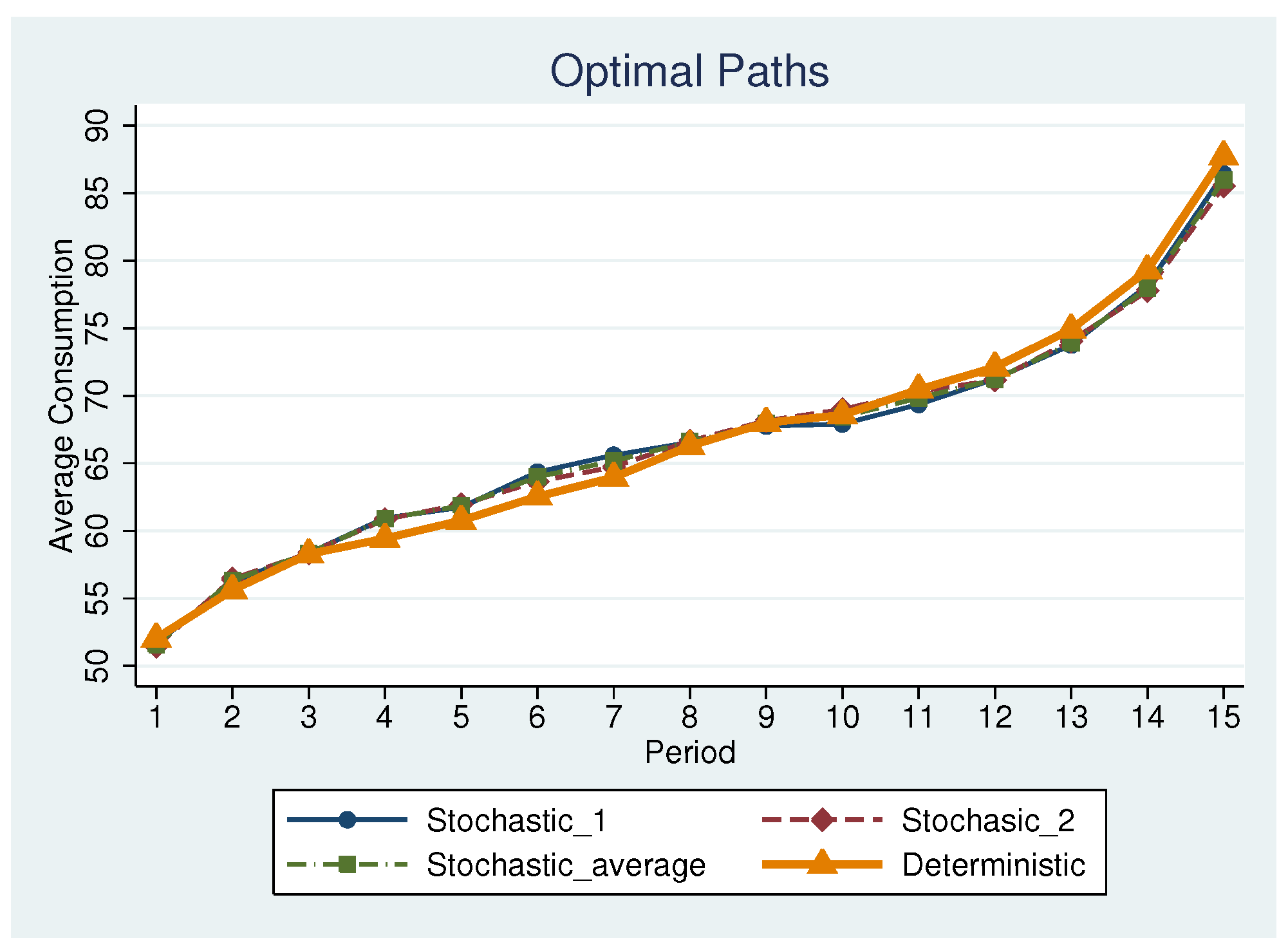
5
For stochastic income, we show the average of the optimal consumption paths for Path 1 and Path 2.
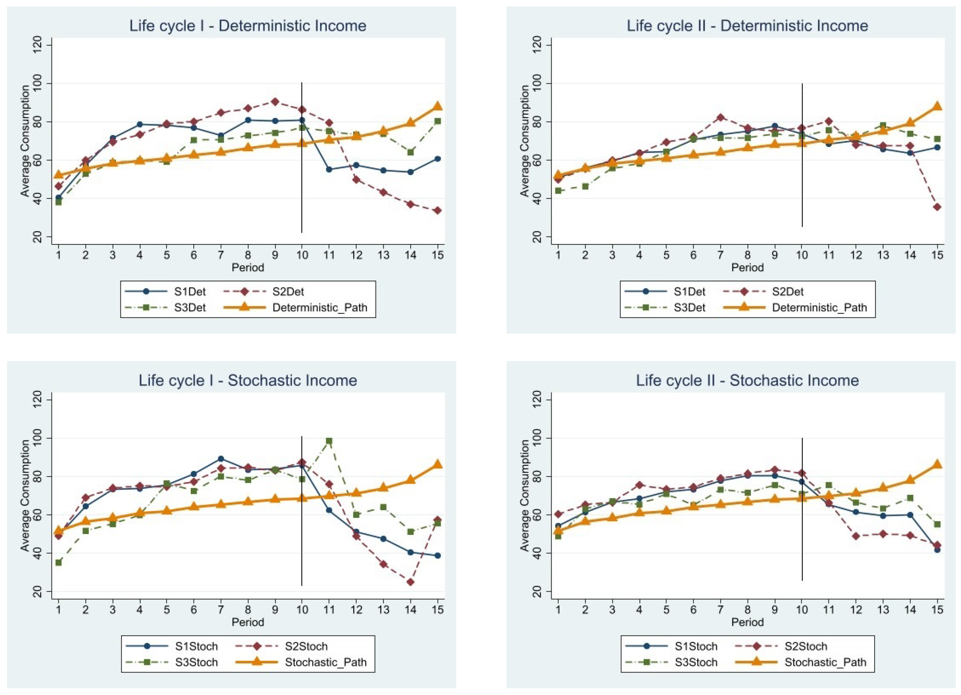
6
For the comparison of observed and optimal paths, we use the average savings across the two life cycles.
7
Descriptive statistics are provided in Appendix C.
8
All regressions are checked for multicollinearity and corrected for heteroscedasticity by using robust standard errors.
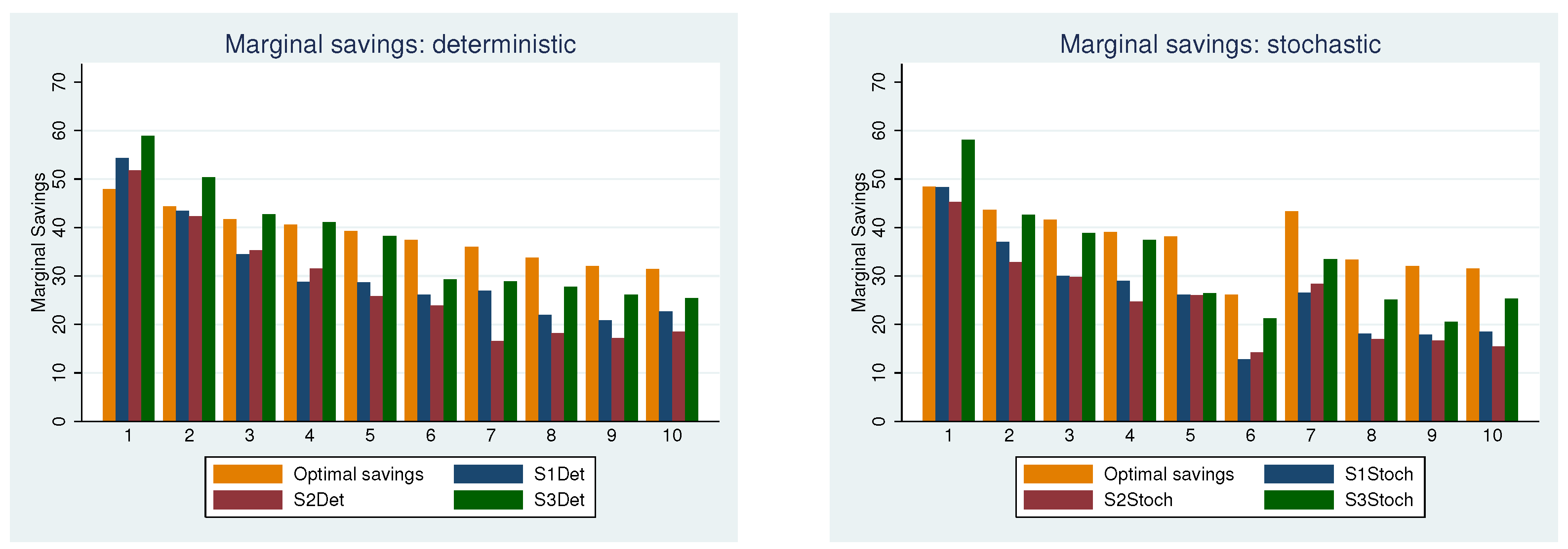
9
These visual conclusions are supported by the results of a Mann–Whitney U-test, see Table A4 and Table A5 in Appendix D. We compare whether (1) pocket savings; (2) the sum of pocket and voluntary savings; and (3) total savings differ across treatments.

References

  1. Agnew, J. R., Anderson, L. R., Gerlach, J. R., & Szykman, L. R. (2008). Who chooses annuities? An experimental investigation of the role of gender, framing, and defaults. American Economic Review, 98(2), 418–422. [Google Scholar] [CrossRef]
  2. Agnew, J. R., Anderson, L. R., & Szykman, L. R. (2015). An experimental study of the effect of market performance on annuitization and equity allocations. Journal of Behavioral Finance, 16(2), 120–129. [Google Scholar] [CrossRef]
  3. Ashraf, N., Karlan, D., & Yin, W. (2006). Tying Odysseus to the Mast: Evidence from a commitment savings product in the philippines. The Quarterly Journal of Economics, 121(2), 635–672. [Google Scholar] [CrossRef]
  4. Bachmann, K., Lot, A., Xu, X., & Hens, T. (2023). Experimental research on retirement decision-making: Evidence from replications. Journal of Banking & Finance, 152, 106851. [Google Scholar]
  5. Ballinger, T. P., Hudson, E., Karkoviata, L., & Wilcox, N. T. (2011). Saving behavior and cognitive abilities. Experimental Economics, 14(3), 349–374. [Google Scholar] [CrossRef]
  6. Ballinger, T. P., Palumbo, M. G., & Wilcox, N. T. (2003). Precautionary saving and social learning across generations: An experiment. The Economic Journal, 113(490), 920–947. [Google Scholar] [CrossRef]
  7. Benartzi, S., & Thaler, R. H. (2013). Behavioral economics and the retirement savings crisis. Science, 339(6124), 1152–1153. [Google Scholar] [CrossRef]
  8. Beshears, J., Choi, J. J., Harris, C., Laibson, D., Madrian, B. C., & Sakong, J. (2015a). Self control and commitment: Can decreasing the liquidity of a savings account increase deposits? (Working Paper No. 21474). National Bureau of Economic Research. Available online: http://www.nber.org/papers/w21474 (accessed on 15 January 2025).
  9. Beshears, J., Choi, J. J., Harris, C., Laibson, D., Madrian, B. C., & Sakong, J. (2020). Which early withdrawal penalty attracts the most deposits to a commitment savings account? Journal of Public Economics, 183, 104144. [Google Scholar] [CrossRef]
  10. Beshears, J., Choi, J. J., Hurwitz, J., Laibson, D., & Madrian, B. C. (2015b). Liquidity in retirement savings systems: An international comparison. American Economic Review, 105(5), 420–425. [Google Scholar] [CrossRef]
  11. Bowman, D., Minehart, D., & Rabin, M. (1999). Loss aversion in a consumption–savings model. Journal of Economic Behavior & Organization, 38(2), 155–178. [Google Scholar]
  12. Brown, A. L., Chua, Z. E., & Camerer, C. F. (2009). Learning and visceral temptation in dynamic saving experiments. The Quarterly Journal of Economics, 124(1), 197–231. [Google Scholar] [CrossRef]
  13. Brown, J. R., Kling, J. R., Mullainathan, S., & Wrobel, M. V. (2008). Why don’t people insure late-life consumption? A framing explanation of the under-annuitization puzzle. American Economic Review, 98(2), 304–309. [Google Scholar] [CrossRef]
  14. Camerer, C. F., & Ho, T.-H. (1994). Violations of the betweenness axiom and nonlinearity in probability. Journal of Risk and Uncertainty, 8(2), 167–196. [Google Scholar] [CrossRef]
  15. Carbone, E., & Hey, J. D. (2004). The effect of unemployment on consumption: An experimental analysis. The Economic Journal, 114(497), 660–683. [Google Scholar] [CrossRef]
  16. Card, D., & Ransom, M. (2011). Pension plan characteristics and framing effects in employee savings behavior. The Review of Economics and Statistics, 93(1), 228–243. [Google Scholar] [CrossRef]
  17. Carroll, C. D. (2000). Solving consumption models with multiplicative habits. Economics Letters, 68(1), 67–77. [Google Scholar] [CrossRef]
  18. Carroll, C. D., Overland, J., & Weil, D. N. (2000). Saving and growth with habit formation. American Economic Review, 90(3), 341–355. [Google Scholar] [CrossRef]
  19. Chen, D. L., Schonger, M., & Wickens, C. (2016). oTree—An open-source platform for laboratory, online, and field experiments. Journal of Behavioral and Experimental Finance, 9, 88–97. [Google Scholar] [CrossRef]
  20. Cleave, B., Nikiforakis, N., & Slonim, R. (2013). Is there selection bias in laboratory experiments? The case of social and risk preferences. Experimental Economics, 16(3), 372–382. [Google Scholar] [CrossRef]
  21. Cohen, J. (1988). Statistical power analysis for the behavioral sciences (2nd ed.). Lawrence Erlbaum Associates. [Google Scholar]
  22. Conway, A. R., Kane, M. J., Bunting, M. F., Hambrick, D. Z., Wilhelm, O., & Engle, R. W. (2005). Working memory span tasks: A methodological review and user’s guide. Psychonomic Bulletin & Review, 12(5), 769–786. [Google Scholar]
  23. Crosetto, P., & Filippin, A. (2013). The “bomb” risk elicitation task. Journal of Risk and Uncertainty, 47, 31–65. [Google Scholar] [CrossRef]
  24. Davidoff, T., Brown, J. R., & Diamond, P. A. (2005). Annuities and individual welfare. American Economic Review, 95(5), 1573–1590. [Google Scholar] [CrossRef]
  25. Duffy, J. (2008). Macroeconomics: A survey of laboratory research. Handbook of Experimental Economics, 2, 1–90. [Google Scholar]
  26. Duffy, J., & Li, Y. (2019). Lifecycle consumption under different income profiles: Evidence and theory. Journal of Economic Dynamics and Control, 104, 74–94. [Google Scholar] [CrossRef]
  27. Duffy, J., & Orland, A. (2023). Liquidity constraints, income variance, and buffer stock savings: Experimental evidence [Unpublished manuscript]. University of California. Irvine, CA, USA.
  28. Ebbinghaus, B. (2021). Inequalities and poverty risks in old age across Europe: The double-edged income effect of pension systems. Social Policy & Administration, 55(3), 440–455. [Google Scholar]
  29. Falk, A., & Heckman, J. J. (2009). Lab experiments are a major source of knowledge in the social sciences. Science, 326(5952), 535–538. [Google Scholar] [CrossRef]
  30. Fatás, E., Lacomba, J. A., Lagos, F., & Moro-Egido, A. I. (2013). An experimental test on dynamic consumption and lump-sum pensions. SERIEs, 4(4), 393–413. [Google Scholar] [CrossRef]
  31. Fehr, E., & Zych, P. K. (1998). Do addicts behave rationally? The Scandinavian Journal of Economics, 100(3), 643–661. [Google Scholar] [CrossRef]
  32. Feltovich, N., & Ejebu, O.-Z. (2014). Do positional goods inhibit saving? Evidence from a life-cycle experiment. Journal of Economic Behavior & Organization, 107, 440–454. [Google Scholar]
  33. Fenig, G., & Petersen, L. (2024). Dynamic optimization meets budgeting: Unraveling financial complexities. NBER Working Paper, 32821, 1–55. [Google Scholar]
  34. Fréchette, G. R. (2015). Laboratory experiments: Professionals versus students. In J. H. Kagel, & A. E. Roth (Eds.), The handbook of experimental economics (Vol. 2, pp. 435–480). Princeton University Press. [Google Scholar]
  35. Friedman, M. (1957). A theory of the consumption function. National Bureau of Economic Research, Inc. [Google Scholar]
  36. Fuhrer, J. C., & Klein, M. W. (1998). Risky habits: On risk sharing, habit formation, and the interpretation of international consumption correlations. National Bureau of Economic Research. [Google Scholar]
  37. Gechert, S., & Siebert, J. (2022). Preferences over wealth: Experimental evidence. Journal of Economic Behavior & Organization, 200, 1297–1317. [Google Scholar]
  38. Gourinchas, P.-O., & Parker, J. A. (2002). Consumption over the life cycle. Econometrica, 70(1), 47–89. [Google Scholar] [CrossRef]
  39. Harris, C., & Laibson, D. (2001). Dynamic choices of hyperbolic consumers. Econometrica, 69(4), 935–957. [Google Scholar] [CrossRef]
  40. Hey, J. D., & Dardanoni, V. (1988). Optimal consumption under uncertainty: An experimental investigation. The Economic Journal, 98(390), 105–116. [Google Scholar] [CrossRef]
  41. Hinrichs, K. (2021). Recent pension reforms in Europe: More challenges, new directions. An overview. Social Policy & Administration, 55(3), 409–422. [Google Scholar]
  42. Karlan, D., McConnell, M., Mullainathan, S., & Zinman, J. (2016). Getting to the top of mind: How reminders increase saving. Management Science, 62(12), 3393–3411. [Google Scholar] [CrossRef]
  43. Kappes, H. B., Campbell, R., & Ivchenko, A. (2023). Scarcity and predictability of income over time: Experimental games as a way to study consumption smoothing. Journal of the Association for Consumer Research, 8(4), 391–402. [Google Scholar] [CrossRef]
  44. Lally, P., Van Jaarsveld, C. H., Potts, H. W., & Wardle, J. (2010). How are habits formed: Modelling habit formation in the real world. European Journal of Social Psychology, 40(6), 998–1009. [Google Scholar] [CrossRef]
  45. Lusardi, A. (1999). Information, expectations, and savings for retirement. Behavioral Dimensions of Retirement Economics, 81, 115. [Google Scholar]
  46. Marshall, A. (2005). From Principles of Economics. In Readings in the economics of the division of labor: The classical tradition (pp. 195–215). World Scientific. [Google Scholar]
  47. Meissner, T. (2016). Intertemporal consumption and debt aversion: An experimental study. Experimental Economics, 19(2), 281–298. [Google Scholar] [CrossRef]
  48. Modigliani, F., & Brumberg, R. (1954). Utility analysis and the consumption function: An interpretation of cross-section data. Post-Keynesian economics, 1, 388–436. [Google Scholar]
  49. Rha, J.-Y., Montalto, C. P., & Hanna, S. D. (2006). The effect of self-control mechanisms on household saving behavior. Journal of Financial Counseling and Planning, 17(2). [Google Scholar]
  50. Rodríguez, C., & Saavedra, J. (2015). Nudging youth to develop savings habits: Experimental evidence using SMS messages. In CESR-schaeffer working paper (2015–2018). Washington University in St. Louis. [Google Scholar]
  51. Rudolph, H. P. (2016). Building voluntary pension schemes in emerging economies. World Bank Policy Research Working Paper. Available online: https://papers.ssrn.com/sol3/papers.cfm?abstract_id=2895485 (accessed on 10 April 2025).
  52. Skinner, J. (1988). Risky income, life cycle consumption, and precautionary savings. Journal of Monetary Economics, 22(2), 237–255. [Google Scholar] [CrossRef]
  53. Thaler, R. H. (1994). Psychology and savings policies. The American Economic Review, 84(2), 186–192. [Google Scholar]
  54. Tversky, A., & Fox, C. R. (1995). Weighing risk and uncertainty. Psychological Review, 102(2), 269. [Google Scholar] [CrossRef]
  55. Tversky, A., & Kahneman, D. (1992). Advances in prospect theory: Cumulative representation of uncertainty. Journal of Risk and Uncertainty, 5(4), 297–323. [Google Scholar] [CrossRef]
  56. Wu, G., & Gonzalez, R. (1996). Curvature of the probability weighting function. Management Science, 42(12), 1676–1690. [Google Scholar] [CrossRef]
  57. Zeldes, S. P. (1989). Optimal consumption with stochastic income: Deviations from certainty equivalence. The Quarterly Journal of Economics, 104(2), 275–298. [Google Scholar] [CrossRef]
Figure 1. Optimal absolute consumption by income path.
Jrfm 18 00240 g001
Figure 2. Average consumption across settings and life cycles. Top: deterministic income, bottom: stochastic income, left: life cycle I, right: life cycle II.
Jrfm 18 00240 g002
Figure 3. Marginal savings: Optimal values vs. values observed in the experiment across treatments. Values shown are averages across stochastic income paths and life cycles.
Jrfm 18 00240 g003
Figure 4. Marginal Savings: S1Det, S2Det, S3Det.
Jrfm 18 00240 g004
Figure 5. Marginal Savings: S1Stoch, S2Stoch, S3Stoch.
Jrfm 18 00240 g005
Table 1. Treatment overview. A + symbol signals that a savings mechanism is available.
SessionTreatmentIncome y t per Period (ECU)SettingPocket SavingsObligatory SavingsVoluntary Savings
1S1Detalways 1001+
2S2Detalways 1002++
3S3Detalways 1003+++
4S1Stoch80, 100 or 1201+
5S2Stoch80, 100 or 1202++
6S3Stoch80, 100 or 1203+++
Table 2. Distribution of characteristics in our sample.
ParameterDescriptionFraction χ 2
GenderFemale/Male61%/39%0.51
EducationHigh School/Bachelor/Master/PhD/Other3%/50%/35%/11%/1%0.40
AgeBelow 20/20–25/25–30/Above 303%/56%/28%/13%0.13
Cognitive abilitiesFewer than 4 correct answers/4–8/8–161%/13%/86%0.39
BackgroundNo /A bit/Some/Sufficient89%/8%/1%/2%0.64
Task UnderstandingNone correct/All Correct18%/82%0.32
Table 3. Average savings at the end of working life across life cycles I and II (ECU).
Deterministic IncomeStochastic Income
S1Det S2Det S3Det Opt S1Stoch S2Stoch S3Stoch Opt
Total308281369384264250329379
Std. Dev.10.6311.9911.425.3910.559.7311.707.03
Table 4. Statistical tests: Total savings (p-values).
Deterministic IncomeStochastic Income
Test Comparison S1Det S2Det S3Det S1Stoch S2Stoch S3Stoch
Mann–Whitney UObserved vs. Optimal0.070.000.630.000.000.02
Wilcoxon-Signed-RankLife cycle I vs. II0.000.000.170.000.000.04
Table 5. Total points collected—Life cycle I and II.
Dependent Variable:
Total Points I Total Points II Δ Total PointsI,II
(1) (2) (3) (4) (5) (6)
Constant1111.259 ***948.928 ***1162.206 ***1096.978 ***50.956 **148.050 ***
(29.491)(66.566)(21.347)(51.644)(20.441)(54.061)
Stochastic−70.925 **−70.772 ***−59.611 ***−61.741 ***11.3149.031
(28.382)(27.291)(20.477)(19.770)(21.262)(20.837)
Setting 2−12.671−28.0502.983−12.38915.65415.661
(29.591)(30.106)(25.719)(24.730)(21.980)(21.997)
Setting 3−32.104−45.6778.199−3.92440.30441.753
(39.313)(37.242)(25.829)(24.497)(28.241)(27.907)
Logic 15.134 *** 8.996 ** −6.137
(5.311) (3.678) (4.215)
Female −41.167 −67.969 *** −26.801
(29.121) (20.213) (22.920)
Observations175175175175175175
R20.0320.1010.0480.1330.0150.043
Note: * p < 0.1; ** p < 0.05; *** p < 0.01.
Table 6. Total points collected—Life cycle I and II using Equation (5).
Dependent Variable:
Total Points ITotal Points II
Constant1253.44 ***1136.03 ***1207.71 ***1128.50 ***
(33.164)(74.812)(27.118)(58.04)
S3_Deterministic46.38 **37.98 *24.7511.90
(20.47)(20.39)(20.85)(20.42)
St.deviation_marginal savings−10.91 ***−10.44 ***−5.106 ***−5.20 ***
(−1.91)(2.04)(1.56)(1.54)
Logic 8.92 * 9.20 **
(4.84) (3.80)
Female −9.99 −60.73 ***
(26.84) (19.92)
N175175175175
R-squared0.2930.3110.0840.161
Note: * p < 0.1; ** p < 0.05; *** p < 0.01.
Disclaimer/Publisher’s Note: The statements, opinions and data contained in all publications are solely those of the individual author(s) and contributor(s) and not of MDPI and/or the editor(s). MDPI and/or the editor(s) disclaim responsibility for any injury to people or property resulting from any ideas, methods, instructions or products referred to in the content.

