Variational Autoencoders for Completing the Volatility Surfaces

Abstract

Variational autoencoders (VAEs) have emerged as a promising tool for modeling volatility surfaces, with particular significance for generating synthetic implied volatility scenarios that enhance risk management capabilities. This study evaluates VAE performance using synthetic volatility surfaces, chosen specifically for their arbitrage-free properties and clean data characteristics. Through a comprehensive comparison with traditional methods including thin-plate spline interpolation, parametric models (SABR and SVI), and deterministic autoencoders, we demonstrate that our VAE approach with latent space optimization consistently outperforms existing methods, particularly in scenarios with extreme data sparsity. Our findings show that accurate, arbitrage-free surface reconstruction is achievable using only 5% of the original data points, with errors 7–12 times lower than competing approaches in high-sparsity scenarios. We rigorously validate the preservation of critical no-arbitrage conditions through probability distribution analysis and total variance strip non-intersection tests. The framework we develop overcomes traditional barriers of limited market data by generating over 13,500 synthetic surfaces for training, compared to typical market availability of fewer than 100. These capabilities have important implications for market risk analysis, derivatives pricing, and the development of more robust risk management frameworks, particularly in emerging markets or for newly introduced derivatives where historical data are scarce. Our integration of machine learning with financial theory constraints represents a significant advancement in volatility surface modeling that balances statistical accuracy with financial relevance.

1. Introduction

Volatility surfaces stand as one of the most critical constructs in modern quantitative finance, providing a multidimensional representation of market-implied volatilities across different strike prices and maturities. These surfaces encapsulate market participants’ expectations of future price movements and serve as fundamental inputs for derivative pricing, risk management, and trading strategies. However, volatility surfaces in real markets frequently suffer from data sparsity issues—missing data points due to illiquid options, limited market depth, or technological constraints in data collection.

1.1. Background and Motivation

The challenge of incomplete volatility surfaces has been a persistent problem in financial markets, particularly in emerging economies, newly listed derivatives, and during periods of market stress. Traditional approaches to surface completion have relied primarily on parametric models (Dumas et al., 1998; Gatheral, 2006) or interpolation techniques (Cont & Vuletić, 2023; Fengler, 2009), which often struggle to capture the complex dynamics of volatility surfaces while maintaining essential no-arbitrage conditions.

The Black–Scholes–Merton model (Black & Scholes, 1973) revolutionized option pricing by providing a closed-form solution under idealized market assumptions. However, real market option prices exhibit systematic deviations from Black–Scholes predictions, manifesting as volatility smiles, skews, and term structures. These patterns reflect market frictions, risk preferences, and anticipation of extreme events that the original Black–Scholes framework does not accommodate (Dupire, 1994; Heston, 1993).

Stochastic volatility models, such as those proposed by Heston (1993) and Bates (1996), and later extended by Christoffersen et al. (2009), have gained prominence for their ability to generate realistic volatility surfaces. However, these models often require sophisticated calibration procedures and may still struggle with fitting market data across all strikes and maturities simultaneously (Andersen & Andreasen, 2000; Gatheral et al., 2020).

1.2. Machine Learning Approaches in Volatility Modeling

Recent advances in machine learning have opened new avenues for modeling financial derivatives and their associated volatility surfaces. Deep learning approaches offer promising alternatives to traditional parametric models, potentially capturing complex, non-linear relationships without imposing restrictive structural assumptions.

Neural network applications in volatility modeling have evolved significantly in recent years. Early work by Hutchinson et al. (1994) demonstrated the potential of neural networks for option pricing, while more recent studies by Ferguson and Green (2018) and Liu et al. (2019) have applied various architectures to predict and model implied volatility. Particularly relevant to our study, Horvath et al. (2021) used deep learning to enforce the absence of static arbitrage in volatility surface modeling, while McGhee (2018) developed neural network architectures specifically designed to satisfy no-arbitrage constraints.

Generative models represent a particularly promising class of machine learning approaches for volatility surface modeling. These models learn the underlying distribution of data to generate new, realistic samples rather than simply mapping inputs to outputs. Notable applications in finance include the work of Wiese et al. (2019) on generative adversarial networks for synthetic financial time series and Kondratyev and Schwarz (2019) on deep generative models for market simulation.

1.3. Variational Autoencoders in Financial Mathematics

Variational autoencoders (VAEs), introduced by Kingma and Welling (2013), represent a powerful class of generative models that combine the strengths of deep learning with probabilistic inference. Unlike deterministic autoencoders, VAEs learn a probability distribution over the latent space, enabling them to generate diverse, realistic samples and quantify uncertainty—properties particularly valuable in financial applications.

The application of VAEs to financial problems has gained momentum in recent years. Takahashi et al. (2019) employed VAEs for anomaly detection in financial time series, while Cao et al. (2020) demonstrated their effectiveness in modeling yield curves. Most directly related to our work, Bergeron et al. (2021) pioneered the use of VAEs for volatility surface modeling, demonstrating their potential for capturing the complex dynamics of these surfaces.

Building upon this foundation, our research makes several significant contributions to the field of volatility surface modeling using VAEs. We develop a comprehensive framework for generating synthetic, arbitrage-free volatility surfaces using parameterized Heston models, creating a robust training dataset that overcomes the limitations of sparse market data. We extend previous latent space optimization approaches by demonstrating successful reconstruction with up to 96% missing data points while maintaining essential mathematical properties. We implement rigorous arbitrage validation procedures, preserving critical no-arbitrage conditions, including calendar spread and butterfly arbitrage constraints. We provide a detailed comparative analysis against established baseline methods, including traditional parametric models, interpolation techniques, and alternative machine learning approaches. Our work integrates machine learning with financial mathematics, addressing the practical challenges of volatility surface completion while respecting the theoretical constraints that make these surfaces economically meaningful.

1.4. Paper Organization

The remainder of this paper is organized as follows: Section 2 provides an overview of generative modeling, with particular emphasis on the mathematical foundations of variational autoencoders. Section 3 details the mathematical framework of VAEs. Section 4 reviews the relevant option pricing theory and the properties of implied volatility surfaces, including no-arbitrage conditions. Section 5 presents our comprehensive research design with comparative baselines. Section 6 details our methodology, including VAE architecture, synthetic data generation, and latent space optimization for surface completion. Section 7 presents our experimental results, evaluating the performance of our approach across various metrics and market scenarios. Finally, Section 8 concludes with a discussion of implications and directions for future research.

Having established the context and goals of our research, we now turn to examine the fundamental concepts of generative modeling that underpin our methodology.

2. What Is Generative Modeling?

Generative modeling is a subfield of machine learning that focuses on learning the underlying distribution of a dataset in order to generate new data points that are statistically similar to the original data. Unlike discriminative models, which aim to classify or predict outcomes based on input features, generative models seek to understand how the data are generated. This understanding allows them to create new instances that can be used for various applications, such as data augmentation, anomaly detection, and simulation.

2.1. Definition and Purpose

At its core, generative modeling involves estimating the joint probability distribution ($P(X,Y)$) of the input data (X) and the corresponding labels (Y). By learning this distribution, generative models can generate new samples ($X^{\prime }$) that resemble the original dataset. The primary purpose of generative modeling is to capture the complex relationships and structures within the data, enabling the generation of realistic and diverse samples.

2.2. Types of Generative Models

Generative models encompass various categories, each with its unique methodology and practical applications. Gaussian mixture models (GMMs) are probabilistic models that assume that the data are generated from a mixture of several Gaussian distributions. They are commonly used for clustering and density estimation. Hidden Markov models (HMMs) are used for modeling sequential data, where the system is assumed to be a Markov process with hidden states, They are mostly utilized in speech recognition and bioinformatics. Generative adversarial networks (GANs), as introduced by Goodfellow et al. (2014), comprise two neural networks, a generator and a discriminator, trained simultaneously. The generator creates synthetic data, while the discriminator evaluates their authenticity. This adversarial training process leads to the generation of highly realistic samples. Variational autoencoders (VAEs), introduced by Kingma and Welling (2013), amalgamate autoencoder and variational inference principles, learning a probabilistic correlation from input data to a latent space for generating new samples. Lastly, normalizing flows represent a class of generative models converting a simple distribution, like Gaussian, into a more intricate form using invertible transformations to enable precise likelihood estimation and proficient sampling.

Generative models are widely used in various fields, serving multiple purposes. They can expand training datasets to enhance supervised learning models, particularly in data-scarce settings. Additionally, generative models excel at detecting anomalies by recognizing data outliers. They are instrumental in producing realistic images and videos, fostering applications in art, entertainment, and virtual reality realms. Moreover, in natural language processing, these models facilitate the generation of coherent text for chatbots, content creation automation, and language translation. Furthermore, in finance, generative models play a significant role in simulating market scenarios, generating synthetic financial data, and modeling intricate financial instruments.

While generative models provide a broad framework for data generation, we now focus specifically on variational autoencoders, which form the cornerstone of our approach to volatility surface modeling.

3. Mathematical Intuition of Variational Autoencoders

Variational autoencoders (VAEs) are a powerful class of generative models that combine principles from deep learning and Bayesian inference. The mathematical intuition behind VAEs lies in their ability to learn a probabilistic representation of the data, allowing the generation of new samples by sampling from a learned latent space. This section will provide a detailed mathematical development of the VAE model, including its formulation, loss function, and the inference process. The VAE architecture is presented in the diagram in Figure 1.

3.1. The Generative Process

In a VAE, we assume that the observed data ($\mathbf{x}$) are generated from some latent variables ($\mathbf{z}$) through a generative process. The generative model can be expressed as follows:

$$p\left(\mathbf{x}\right|\mathbf{z})=\mathcal{N}(\mathbf{x};\mu \left(\mathbf{z}\right),{\sigma }^2\left(\mathbf{z}\right))$$

(1)

where $\mu \left(\mathbf{z}\right)$ and (${\sigma }^2\left(\mathbf{z}\right)$) are the parameters of the output distribution, typically modeled by a neural network. The latent variables ($\mathbf{z}$) are assumed to follow a prior distribution:

$$p\left(\mathbf{z}\right)=\mathcal{N}(\mathbf{z};\mathbf{0},\mathbf{I})$$

(2)

where ($\mathbf{I}$) is the identity matrix, indicating that the latent variables are drawn from a standard normal distribution.

3.2. The Inference Process

The goal of a VAE is to learn the posterior distribution ($p\left(\mathbf{z}\right|\mathbf{x})$), which is typically intractable. Instead, we approximate this posterior using a variational distribution ($q\left(\mathbf{z}\right|\mathbf{x})$), which is also modeled by a neural network. The variational distribution is parameterized by ($\mathit{\varphi }$):

$$q\left(\mathbf{z}\right|\mathbf{x})=\mathcal{N}(\mathbf{z};{\mu }_{\varphi }\left(\mathbf{x}\right),{\sigma }_{\varphi }^2\left(\mathbf{x}\right))$$

(3)

where (${\mu }_{\varphi }\left(\mathbf{x}\right)$) and (${\sigma }_{\varphi }^2\left(\mathbf{x}\right)$) are the outputs of the encoder network.

3.3. The Evidence Lower Bound (ELBO)

To train the VAE, we maximize the marginal likelihood of the data ($p\left(\mathbf{x}\right)$). However, as this is often intractable, we instead maximize the evidence lower bound (ELBO), which can be expressed as

$$logp\left(\mathbf{x}\right)\ge {\mathbb{E}}_{q\left(\mathbf{z}\right|\mathbf{x})}\left[logp\left(\mathbf{x}\right|\mathbf{z})\right]-D_{KL}\left(q\left(\mathbf{z}\right|\mathbf{x})\right|\left|p\left(\mathbf{z}\right)\right)$$

(4)

where ($D_{KL}$) is the Kullback–Leibler divergence, measuring the difference between the variational distribution ($q\left(\mathbf{z}\right|\mathbf{x})$) and the prior ($p\left(\mathbf{z}\right)$).

The ELBO can be rewritten as

$$\mathcal{L}(\mathbf{x};\mathit{\varphi },\mathit{\theta })={\mathbb{E}}_{q\left(\mathbf{z}\right|\mathbf{x})}\left[logp\left(\mathbf{x}\right|\mathbf{z})\right]-D_{KL}\left(q\left(\mathbf{z}\right|\mathbf{x})\right|\left|p\left(\mathbf{z}\right)\right)$$

(5)

The first term, $\left({\mathbb{E}}_{q\left(\mathbf{z}\right|\mathbf{x})}\left[logp\left(\mathbf{x}\right|\mathbf{z})\right]\right)$, represents the expected log-likelihood of the data given the latent variables, while the second term, $(D_{KL}\left(q\left(\mathbf{z}\right|\mathbf{x})\right|\left|p\left(\mathbf{z}\right)\right))$, acts as a regularization term that encourages the variational distribution to be close to the prior distribution.

3.4. The Loss Function

To optimize the VAE, we minimize the negative ELBO, which can be expressed as the loss function:

$$\mathcal{L}(\mathbf{x};\mathit{\varphi },\mathit{\theta })=-{\mathbb{E}}_{q\left(\mathbf{z}\right|\mathbf{x})}\left[logp\left(\mathbf{x}\right|\mathbf{z})\right]+D_{KL}\left(q\left(\mathbf{z}\right|\mathbf{x})\right|\left|p\left(\mathbf{z}\right)\right)$$

(6)

This loss function consists of two components:

• Reconstruction loss: The first term measures how well the model can reconstruct the input data from the latent representation.
• Regularization loss: The second term penalizes the divergence between the variational distribution and the prior distribution, ensuring that the learned latent space follows the desired prior distribution (standard normal distribution).

3.5. Sampling from the Latent Space

Once the VAE is trained, we can generate new samples by sampling from the prior distribution ($p\left(\mathbf{z}\right)$) and passing the samples through the decoder network:

Sample ($\mathbf{z}$) from the prior:

$$\mathbf{z}\sim p\left(\mathbf{z}\right)=\mathcal{N}(\mathbf{z};\mathbf{0},\mathbf{I})$$

(7)

Generate new data (${\mathbf{x}}^{\prime }$) from the decoder:

$${\mathbf{x}}^{\prime }\sim p\left(\mathbf{x}\right|\mathbf{z})$$

(8)

This process allows the VAE to generate new data points that are consistent with the learned distribution of the training data.

With the mathematical foundations of VAEs established, we now explore the financial context of our application by examining option pricing theory and the properties of implied volatility surfaces.

4. Option Pricing and Implied Volatility

Implied volatility (IV) is a critical concept in options pricing and financial markets analysis. It represents the market’s forecast of likely price movements of an underlying asset, derived from option prices rather than historical price data. This overview explores the theoretical foundations, practical applications, and mathematical frameworks of implied volatility. The concept of implied volatility emerged from the Black–Scholes–Merton option pricing model (Black & Scholes, 1973). While the original Black–Scholes formula uses volatility as an input to determine option prices, implied volatility reverses this process by using market option prices to derive the volatility parameter.

The Black–Scholes formula for a European call option is given by

$$C(S,t)=S_{0}N\left(d_1\right)-K{e}^{-rT}N\left(d_2\right)$$

(9)

where

$$d_1={\displaystyle \frac{ln(S_0/K)+(r+{\sigma }^2/2)T}{\sigma \sqrt{T}}}$$

(10)

$$d_2=d_1-\sigma \sqrt{T}$$

(11)

The Implied Volatility surface of an option is the graph of a function whose variables are the time to maturity (T) and the strike price (K) of that option. It can be written as

$$IV=f(T,K)$$

(12)

An implied volatility is the volatility needed in the Black–Scholes Formula (9) to recover the market or model price.

In financial markets, option prices exhibit systematic deviations from Black–Scholes assumptions, particularly volatility smile/skew across strikes, term structure of volatility, and stochastic nature of volatility itself. Under the risk-neutral measure $\mathbb{Q}$, with $S\left(t\right)$ as the asset price and $v\left(t\right)$ as variance, the implied volatility is defined under the Heston model as follows (Heston, 1993):

$$\begin{array}{ccc}\hfill {\displaystyle \frac{dS\left(t\right)}{S\left(t\right)}}& =& (r-q)dt+\sqrt{v\left(t\right)}S\left(t\right)d{W}_1\left(t\right)\hfill \\ \hfill dv\left(t\right)& =& \kappa (\theta -v\left(t\right))dt+\sigma \sqrt{v\left(t\right)}d{W}_2\left(t\right)\hfill \\ \hfill d{\langle W_1,W_2\rangle }_t& =& \rho dt\hfill \end{array}$$

(13)

where

• r: Risk-free rate.
• q: Dividend yield.
• $\kappa$: Speed of mean reversion. A high $\kappa$ means rapid mean reversion, and stable long-dated volatilities.
• $\theta$: Long-term variance.
• $\sigma$: Volatility of variance. A high $\sigma$ means more pronounced volatility smile.
• $\rho$: Correlation coefficient; a negative $\rho$ would depict downward-sloping skew (equity markets) and a positive $\rho$ would indicate an upward-sloping skew (some FX pairs).

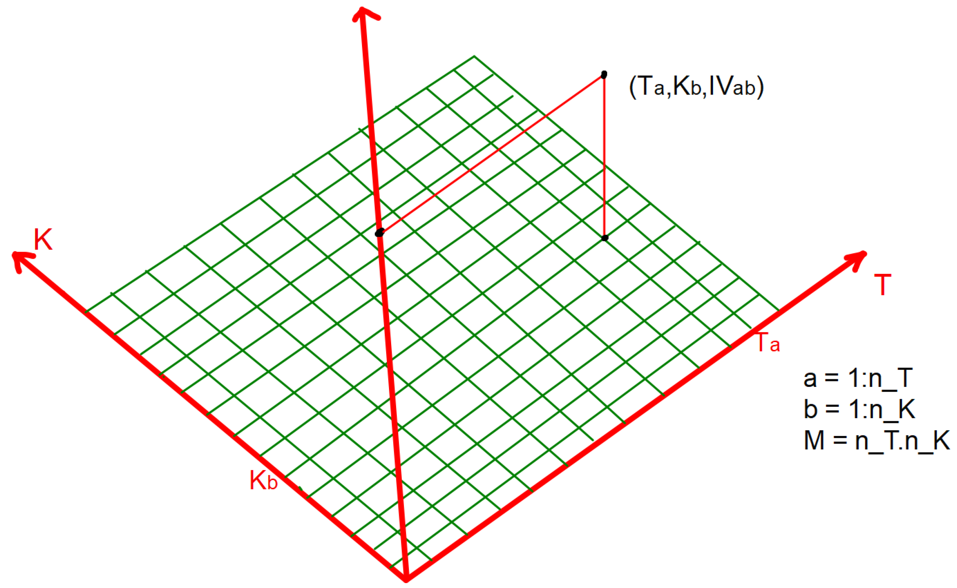
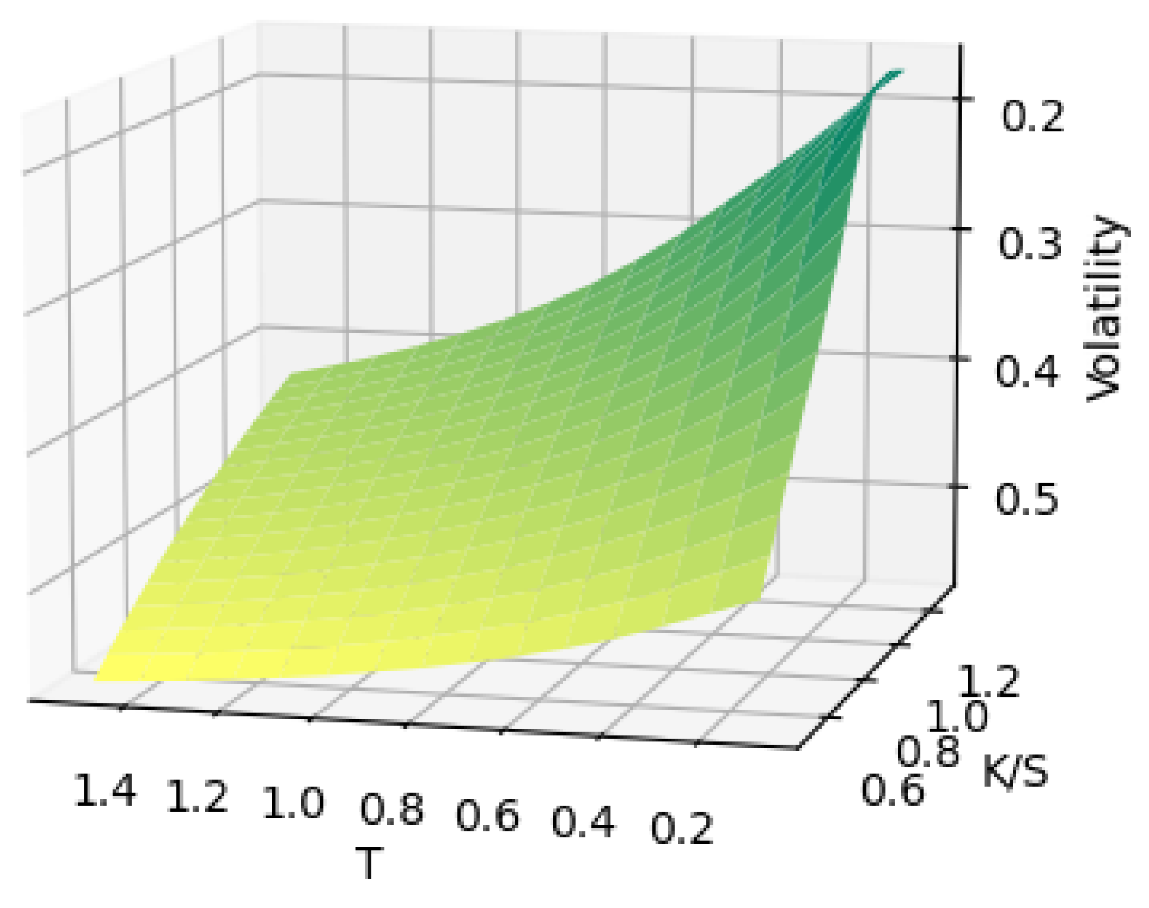
The 5-tuples ($\theta$, $\sigma$, $\kappa$, $\rho$, and $v\left(0\right)$) are randomly generated within a certain range, depending on the asset class and properties of the underlying asset. For each 5-tuple of parameters, we price a call/put option on a fixed $n_T\times n_K$ grid made of maturity dates and strikes. The implied volatilities at grid points are calculated for each 5-tuple of parameters; see Figure 2.

4.1. Feller Condition

The Feller condition states that

$$2\kappa \theta \ge {\sigma }^2$$

(14)

This condition ensures variance remains positive.

This condition is crucial in ensuring that the model for generating volatility surfaces obeys the critical properties of a volatility surface. Implied volatility remains a cornerstone of modern quantitative finance, combining theoretical elegance with practical market applications. Understanding its properties and dynamics is essential for options trading, risk management, and market analysis.

4.2. No-Arbitrage Conditions

Calendar spread arbitrage occurs when there is a discrepancy in option prices between two options with different expiration dates. Specifically, if for two European call options with strikes K and maturities $T_1$ and $T_2$ where $T_1<T_2$, we have

$$C(T_1,K)>C(T_2,K).$$

(15)

Given the fact that we are dealing with volatility surfaces, when we consider calendar arbitrage in terms of forward moneyness $K/F_T$, the graphs of ${\sigma }^2(K,T)$ plotted against T for different $K/F_T$ ratios should not intersect. If two such curves were to meet, it would violate the no-calendar-arbitrage condition as it would imply that the accumulated variance between two time points is the same for different forward moneyness levels. This is inconsistent with arbitrage-free pricing because the forward smile evolution must maintain proper ordering of total variance across different moneyness levels. Mathematically, if we fix $K/F_T=k_1$ and $K/F_T=k_2$ where $k_1\ne k_2$, then the curves $T\to {\sigma }^2(k_1{F}_T,T)$ and $T\to {\sigma }^2(k_2{F}_T,T)$ must never intersect.

Butterfly arbitrage occurs when an opportunist trader can combine call or put options to create riskless profits.

Consider three options with strikes $K-ϵ<K<K+ϵ$.

• Buy one call (or put) option of strike $K-ϵ$.
• Sell two call (or put) option of strike K.
• Buy one call (or put) option of strike $K+ϵ$.

The options above must be of the same type (put or call). Assuming that there is no transaction cost, no market impact, and no risk exposure other than the specific options being traded, it is a market-neutral strategy designed to exploit pricing inefficiencies.

The absence of butterfly arbitrage requires that the implied probability density function (PDF) must be non-negative for all strikes (Fengler, 2009). Starting from the Breeden–Litzenberger formula, the PDF $f\left(K\right)$ is proportional to the second derivative of the call price with respect to strike:

$$f\left(K\right)\propto {\partial }^{2}C/\partial K^2\ge 0$$

(16)

When expressed in terms of implied volatility $\sigma (K,T)$, this non-negativity condition translates to a relationship between the level, slope, and convexity of the volatility smile. For the density to be valid, we need

$${\partial }^{2}C/\partial K^2\ge 0$$

(17)

This condition can be rewritten in terms of implied volatility as

$${\sigma }^{″}\left(K\right)+2{\displaystyle \frac{{\left({\sigma }^{\prime }\left(K\right)\right)}^2}{\sigma \left(K\right)}}+2{\displaystyle \frac{{\sigma }^{\prime }\left(K\right)}{K}}+{\displaystyle \frac{d_1{d}_2}{K\sigma \left(K\right)}}\ge 0$$

(18)

where $d_1$ and $d_2$ are the standard Black–Scholes parameters.

$$\begin{array}{ccc}\hfill d_1& =& {\displaystyle \frac{ln(S/K)+(r+\frac{{\sigma }^2}{2})T}{\sigma \sqrt{T}}}\ge 0\hfill \\ \hfill d_2& =& d_1-\sigma \sqrt{T}\hfill \end{array}$$

(19)

The inequality in Equation (18) ensures that any slice of the volatility surface corresponds to a meaningful probability distribution.

Having outlined both the mathematical framework of VAEs and the financial theory of implied volatility, we now present our research design with comparative baselines before describing our approach to combining these concepts in training a VAE model on synthetic volatility surfaces.

5. Research Design and Comparative Framework

This section outlines our research design, theoretical foundations, and experimental framework. We present a structured approach to investigating the efficacy of variational autoencoders for volatility surface completion, with particular attention to maintaining arbitrage-free properties and comparing against established methods.

5.1. Research Questions and Hypotheses

Our study addresses the following primary research questions:

• Efficacy Question: Can variational autoencoders effectively reconstruct volatility surfaces from sparse data while maintaining essential financial properties?
• Sparsity Limits Question: What is the maximum level of data sparsity at which reliable surface reconstruction remains possible?
• Methodology Question: How does latent space optimization compare to traditional reconstruction approaches for volatility surface completion?
• Arbitrage Question: Do the reconstructed surfaces preserve critical no-arbitrage conditions required for financial applications?

Based on these research questions, we formulate the following hypotheses:

• Hypotheses 1: VAEs can reconstruct complete volatility surfaces with mean squared error below ${10}^{-5}$ when trained on synthetic Heston-generated surfaces.
• Hypotheses 2: Latent space optimization significantly outperforms direct encoder–decoder reconstruction for sparse surfaces, with the performance gap widening as sparsity increases.
• Hypotheses 3: Successful reconstruction is possible with up to 95% missing data points when using latent space optimization techniques.

5.2. Theoretical Framework

Our research integrates three theoretical domains:

5.2.1. Financial Theory of Volatility Surfaces

Volatility surfaces represent the mapping of implied volatilities across option strikes and maturities. These surfaces must satisfy specific mathematical properties to prevent arbitrage opportunities. The key requirements include monotonicity in maturity, where total variance (${\sigma }^{2}T$) must increase with maturity for each strike, and butterfly spread constraints, which ensure the risk-neutral density remains positive by requiring specific constraints on the second derivative of option prices with respect to strike prices. These no-arbitrage conditions serve as critical validation criteria in our research design, ensuring that reconstructed surfaces remain economically meaningful.

5.2.2. Deep Generative Modeling

Our approach leverages variational autoencoders—a class of deep generative models that learn probabilistic mappings between high-dimensional data and low-dimensional latent spaces. The VAE framework offers several advantages for our application:

• Probabilistic representation: VAEs capture uncertainty in the latent representation, essential for financial modeling.
• Regularization: The KL divergence term prevents overfitting and encourages a structured latent space.
• Generative capacity: The learned probability distribution enables generation of new, realistic surfaces.

5.2.3. Latent Space Optimization

We extend standard VAE methodology by implementing latent space optimization—finding the optimal latent vector that, when decoded, best reproduces the known points on a sparse surface. This approach leverages the learned manifold structure of the latent space, constraining solutions to the space of plausible volatility surfaces.

5.3. Experimental Design

Our experimental framework follows a systematic, multi-stage approach:

5.3.1. Data Generation and Preparation

Rather than relying on limited market data, we generate a comprehensive synthetic dataset using the Heston stochastic volatility model. This approach offers several advantages:

• Scale: Generation of thousands of diverse surfaces, far exceeding what would be available from market data.
• Quality control: Guaranteed arbitrage-free properties by construction.
• Parameter diversity: Systematic coverage of different market regimes and volatility patterns.
• Ground truth: Perfect knowledge of the complete surface for validation purposes.

The parameter ranges for our Heston model were carefully calibrated based on an extensive review of the literature (Gatheral, 2006; Christoffersen et al., 2009) and empirical analysis of real market data to ensure realistic behavior.

5.3.2. Evaluation Protocols

To rigorously evaluate our hypotheses, we designed the following experimental protocols:

• Protocol 1: Baseline Reconstruction Evaluation

  -

  Complete surfaces from the test set (not used during training).

  -

  Reconstruction through full encode–decode cycle.

  -

  Metrics: MSE, RMSE, MAE, and financial metrics (pricing errors).

• Protocol 2: Sparse Surface Completion

  -

  Randomly remove points from test surfaces at varying sparsity levels (20%, 40%, 60%, 80%, 96%).

  -

  Compare standard reconstruction (encode–decode with missing values set to zero) vs. latent optimization.

  -

  Metrics: Reconstruction error on known points, error on held-out points, computational time.

• Protocol 3: Arbitrage Validation

  -

  Evaluate calendar spread and butterfly arbitrage conditions.

  -

  Compute risk-neutral density functions from reconstructed surfaces.

5.3.3. Evaluation Metrics

We employ a comprehensive evaluation framework incorporating both statistical and financial metrics:

Statistical Metrics:

• Mean squared error (MSE): Primary metric for overall reconstruction quality.
• Root mean squared error (RMSE): For interpretability in volatility units.
• Mean absolute error (MAE): Less sensitive to outliers than MSE/RMSE.
• Mean absolute percentage error (MAPE): For relative error assessment.

Financial Metrics:

• Option pricing error: Difference in option prices computed using original vs. reconstructed volatilities.
• Risk-neutral density quality: Integrated squared error between original and reconstructed densities.

5.4. Comparative Baselines

To contextualize our results, we implement and evaluate several established baseline approaches:

• Thin-plate spline interpolation: A widely used non-parametric approach for volatility surface interpolation that fits a smooth surface through known data points Webba (1990).
• Deterministic autoencoder: A non-variational version of our approach with identical architecture, allowing us to isolate the benefits of the variational component Hinton and Salakhutdinov (2006).
• Parametric SABR model: The stochastic alpha–beta–rho model Hagan et al. (2002) that fits parameters to match known volatility points and generates a complete surface based on those parameters.
• SVI parameterization: The stochastic volatility inspired approach proposed by Gatheral (2004) that provides a parsimonious parameterization of the volatility surface.

These baselines represent both traditional approaches in industry practice and competing machine learning methodologies, providing a comprehensive benchmark for our VAE-based approach.

5.5. Implementation and Computational Environment

Our experiments were implemented using TensorFlow $2.4$ with custom extensions for financial mathematics. The models were trained on a standard laptop/desktop configuration with the following specifications:

• Hardware: Intel Core $i7-8750HCPU\left(2.20GHz\right)$ with $24GB$ RAM.
• Batch size: 32 (optimized for available memory constraints).
• Training epochs: 100 with early stopping based on validation loss.
• Optimizer: Adam with learning rate $0.001$ and exponential decay.
• Loss function: ELBO with KL annealing schedule.
• Regularization: $L2$ weight decay (coefficient 10⁻⁵) and dropout (rate 0.2).

The moderate hardware requirements demonstrate that our approach is accessible without specialized equipment, making it practical for implementation in typical industry settings. This research design provides a rigorous framework for evaluating our hypotheses while ensuring both statistical validity and financial relevance of our findings.

6. Methodology and Implementation

This section details our comprehensive methodology for volatility surface modeling and completion using VAEs, covering the synthetic data generation process, model architecture, training procedure, and latent space optimization approach.

6.1. Synthetic Data Generation Framework

A key innovation in our approach is the use of synthetic data generated from a well-established stochastic volatility model. This strategy overcomes the limitations of market data, which are often sparse, incomplete, and limited in diversity.

6.1.1. Heston Model Implementation

We employ the Heston stochastic volatility model defined in Equation (13) to generate a diverse set of synthetic volatility surfaces. The Heston model was selected for its ability to capture key market phenomena such as volatility smiles, skews, and term structures, while ensuring theoretical consistency and arbitrage-free properties.

For each generated surface, we use a unique set of five parameters ($v_0$, $\rho$, $\sigma$, $\kappa$, $\theta$) sampled from carefully calibrated distributions that reflect realistic market conditions. These parameter ranges, shown in

Table 1. Parameters of the IV generation framework.

Parameters	${\mathit{v}}_0$	$\mathit{\rho }$	$\mathit{\sigma }$	$\mathit{\theta }$	$\mathit{\kappa }$
Lower bound	0.025	−0.87	0.5	0.08	0.1
Upper bound	0.035	−0.067	1.5	0.1	2.2

, were determined through analysis of historical market data and established research (Gatheral, 2006; Christoffersen et al., 2009).

For each parameter set, we enforce the Feller condition ($2\kappa \theta \ge {\sigma }^2$) to ensure variance positivity and model stability. Additionally, we verify that the resulting surfaces satisfy the no-arbitrage conditions described in Section 4.2.

6.1.2. Surface Discretization and Grid Design

Each volatility surface is generated on a fixed grid with the following specifications:

$$\begin{array}{ccc}\hfill S_0& =& 1.0r=0.0\hfill \\ \hfill T& =& [0.1,0.2,0.3,0.4,0.5,0.6,0.7,0.8,0.9,1.0,1.1,1.2,1.3,1.4,1.5]\hfill \\ \hfill K& =& [0.50,0.55,0.60,0.65,0.7,0.75,0.8,0.85,0.9,0.95,1.0,1.05,1.1,1.15,1.2,1.25,1.30]\hfill \\ \hfill n_T& =& 15,n_K=17M=n_T\times n_K=255\hfill \end{array}$$

(20)

This grid design provides comprehensive coverage of both the term structure (maturities from 0.1 to 1.5 years) and moneyness (strikes from deep in-the-money to deep out-of-the-money). The total of 255 grid points per surface enables detailed representation of complex volatility patterns.

6.1.3. Data Processing and Filtering

We initially generated 20,000 synthetic volatility surfaces. Each surface was subjected to rigorous quality checks:

• Verification of no calendar spread arbitrage using total variance test.
• Validation of no butterfly arbitrage through risk-neutral density calculation.
• Checks for numerical stability and realistic value ranges.

After filtering, we retained 13,500 high-quality, arbitrage-free surfaces. This dataset was then split into training ($80\%$) and testing ($20\%$) sets, ensuring that the test set contained surfaces with parameter combinations not seen during training.

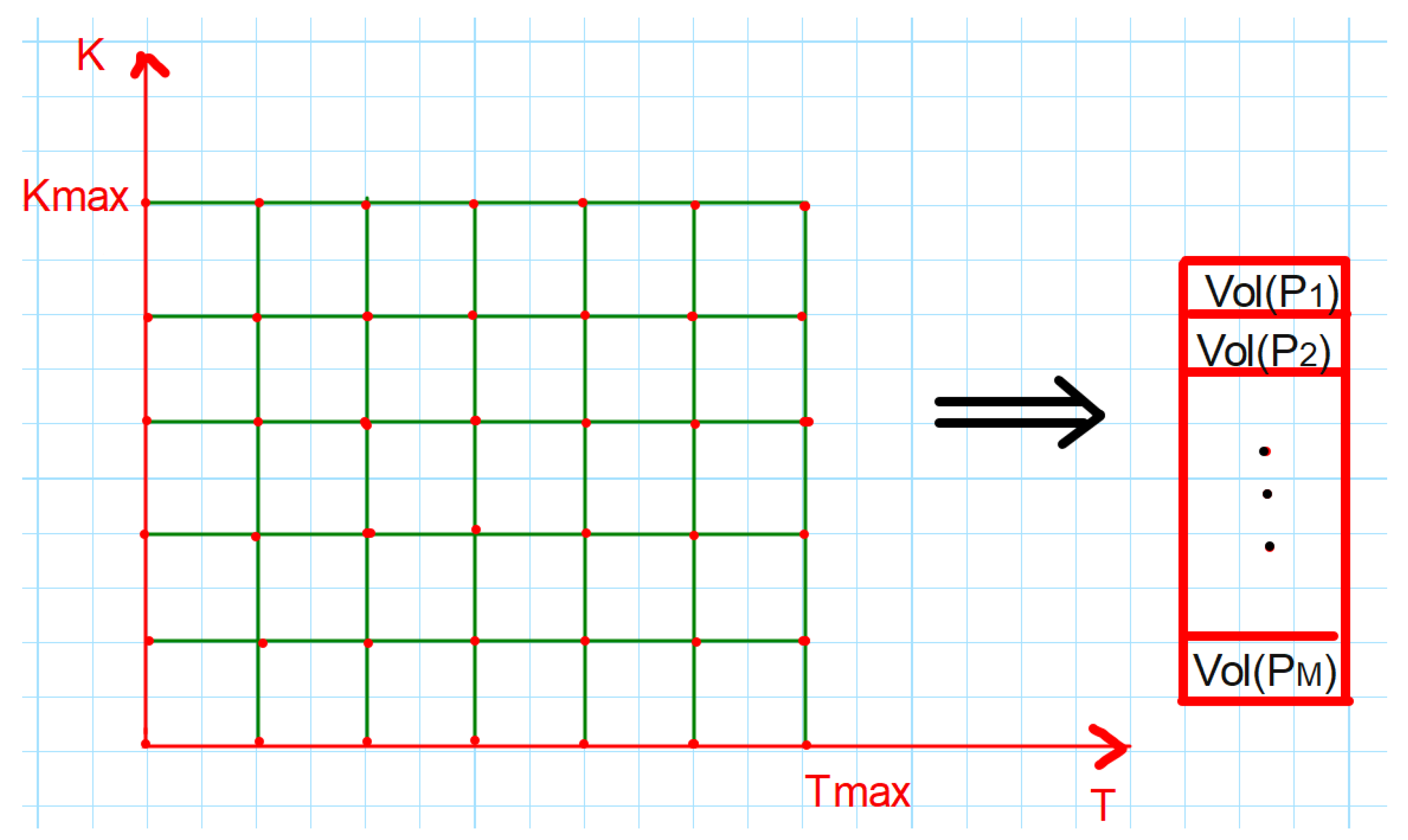
6.2. Data Preprocessing and Representation

6.2.1. Surface Flattening and Normalization

Volatility surfaces are inherently two-dimensional structures, with one dimension corresponding to strike and the other to maturity. To make these surfaces compatible with our neural network architecture, we employed a flattening procedure, illustrated in Figure 3.

Each 2D surface of shape $(n_T,n_K)$ is transformed into a 1D vector of length $n_T\times n_K=255$. This flattened representation preserves all information while creating a format suitable for processing by the VAE.

Prior to training, we normalized the volatility values to the range [0, 1] using min–max scaling, recording the scaling parameters for later denormalization. This normalization improves training stability and helps the model converge more efficiently.

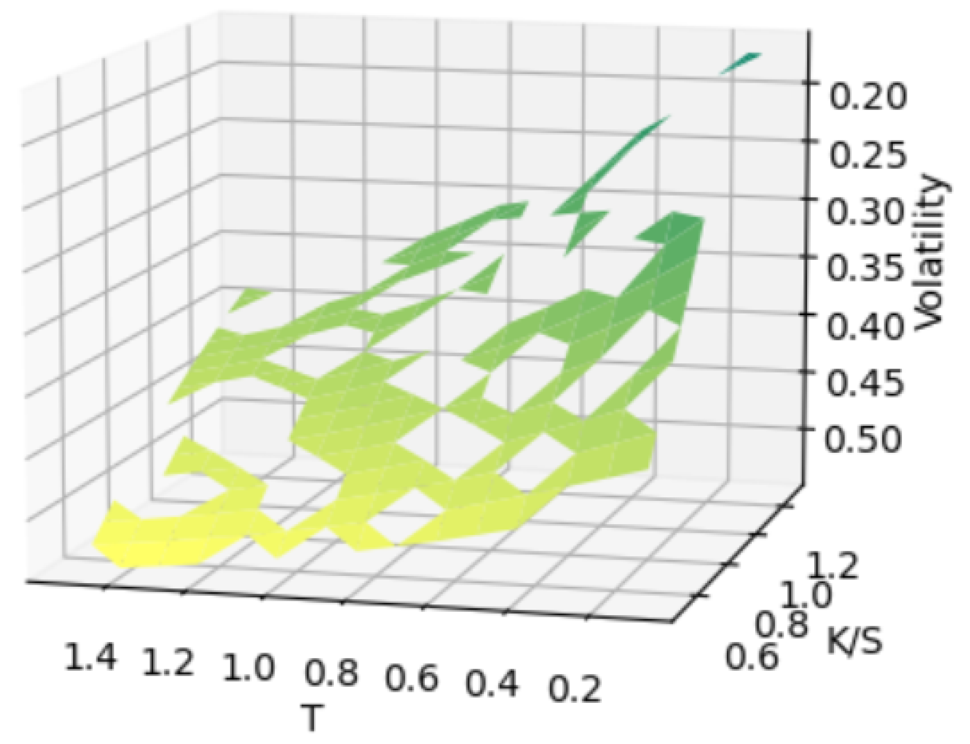
6.2.2. Sparse Surface Simulation

To simulate real-world scenarios with incomplete data, we created partially observed surfaces by randomly removing points from complete surfaces. Figure 4 shows an example of a surface with approximately $40\%$ of points removed.

We systematically varied the percentage of missing points ($20\%$, $40\%$, $60\%$, $80\%$, and $96\%$) to evaluate our method’s performance under different sparsity conditions. For each sparsity level, we generated multiple test cases with different random masks to ensure robust evaluation.

6.3. VAE Architecture and Training

6.3.1. Network Design and Hyperparameters

Our VAE implementation uses a carefully designed architecture optimized for volatility surface representation, as detailed in

Table 2. VAE model architecture specifications.

	VAE Architecture
	Dimension	Activation Function	Number of Batches	Number of Epochs
Encoder	(255, 128, 64, 32)	(elu, elu, elu)	100	100
Latent Space Dim.	16
Decoder	(16, 32, 64, 128, 255)	{elu, elu, elu, sigmoid}

.

The encoder network maps the 255-dimensional input to a 16-dimensional latent space through progressively smaller hidden layers (128, 64, 32 neurons). The decoder mirrors this structure in reverse, reconstructing the 255-dimensional surface from the latent representation.

We used exponential linear unit (ELU) activations throughout the network, except for the decoder output layer, which uses sigmoid activation to constrain values to the [0, 1] range. The latent space dimension of 16 was determined through ablation studies, providing an optimal balance between compression and reconstruction quality.

6.3.2. Training Protocol

The model was trained using the following configuration:

• Optimizer: Adam with learning rate $0.001$ and exponential decay.
• Batch size: 32 (adjusted for our hardware constraints).
• Training epochs: 100 with early stopping based on validation loss.
• Loss function: $ELBO$ with $KL$ annealing schedule to prevent posterior collapse.
• Regularization: $L2$ weight decay (coefficient 10⁻⁵) and dropout (rate 0.2).

The KL annealing schedule gradually increases the weight of the KL divergence term in the loss function from 0 to 1 over the first 10 epochs. This approach helps prevent posterior collapse, a common issue in VAE training where the model ignores the latent space and relies solely on the decoder’s capacity.

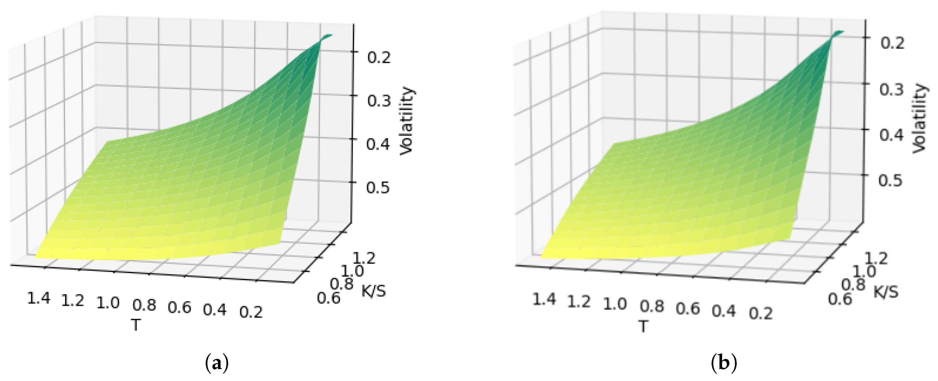
6.4. Evaluation of Reconstruction Performance

Figure 5 compares an original Heston-generated surface with its VAE reconstruction, demonstrating the model’s ability to accurately capture the complex structure of volatility surfaces.

7. Results and Analysis

This section presents the experimental results of our approach, including both the standard VAE reconstruction and our enhanced latent space optimization method. We evaluate performance across different sparsity levels and compare against established baseline methods.

7.1. Surface Completion via Latent Space Optimization

7.1.1. Optimization Framework

We formulate the volatility surface completion problem as an optimization in the VAE’s latent space. Given a partially observed volatility surface with missing values, we seek to find the optimal latent vector $Z^{★}$ that, when passed through the decoder, produces a surface that best matches the known points while generating plausible values for the missing points.

This optimization can be formalized as follows:

$$Z^{★}={\mathrm{argmin}}_z\Vert \mathrm{decoder}\left(z\right)-{\mathrm{target}\Vert }^2$$

(21)

where the target contains the known points of the incomplete surface, and the error is computed only over these known points. This approach leverages the learned manifold structure of the latent space, constraining the solution to the space of realistic volatility surfaces.

7.1.2. Implementation and Results

We begin with a complete Heston volatility surface from the test set and randomly remove points to create a sparse surface. Figure 6 shows an example with approximately $40\%$ (100 points) removed, reconstructed using the standard VAE approach (direct encode-decode with zeros in place of missing values).

Figure 7 shows the same surface reconstructed using our latent space optimization approach. The visual improvement is evident, with the optimization approach producing a smoother, more realistic surface.

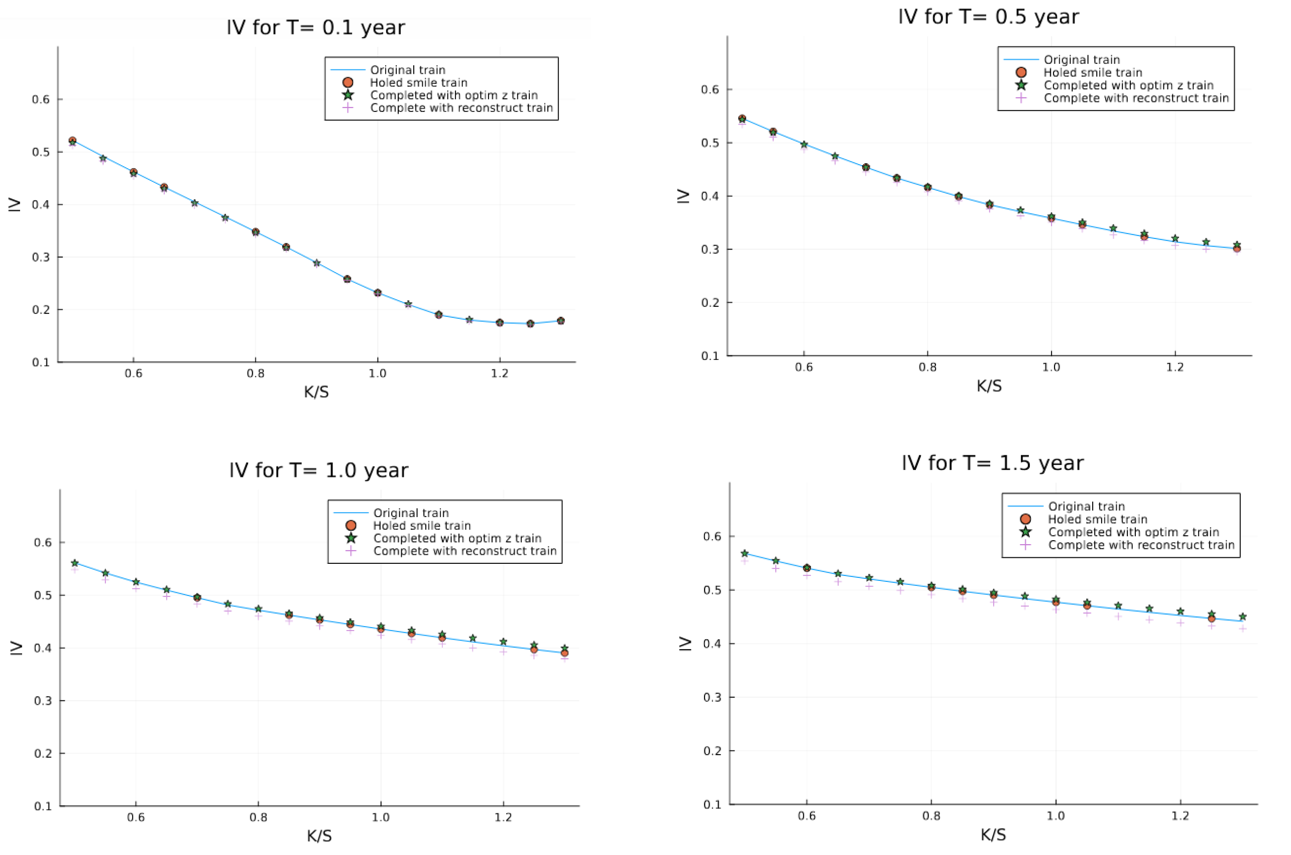
For more detailed evaluation, Figure 8 displays volatility slices at selected maturities, comparing the original surface, the incomplete surface, and our reconstruction.

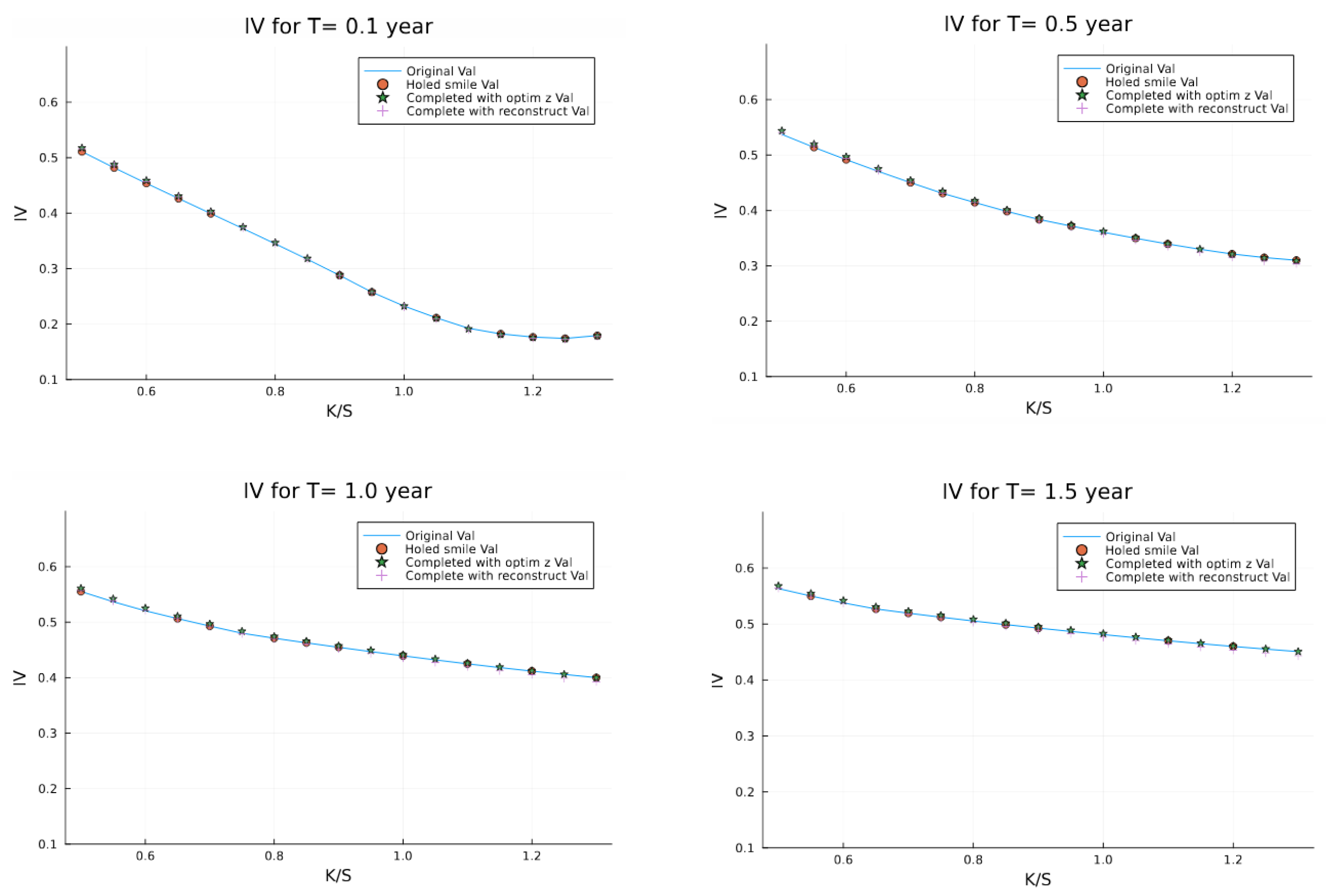
Similarly, Figure 9 shows results on the validation set, demonstrating the generalization capability of our approach to surfaces not seen during training.

7.2. Quantitative Performance Analysis

Table 3. Comparison of reconstruction errors between standard reconstruction and latent optimization approaches for different percentages of missing data points.

% Holes	Nbr of Holes	Training Set		Validation Set
		Error Recons	Error Latent Opt	Error Recons	Error Latent Opt
20%	51	6.59 × 10−6	3.71 × 10−6	3.619 × 10−5	3.616 × 10−5
40%	102	6.59 × 10−6	3.91 × 10−6	3.62 × 10−5	3.616 × 10−5
60%	153	6.59 × 10−6	4.39 × 10−6	3.621 × 10−5	3.617 × 10−5
80%	204	1.008 × 10−5	5.40 × 10−6	3.621 × 10−5	3.617 × 10−5
96%	243	1.95 × 10−5	5.21 × 10−6	3.622 × 10−5	3.617 × 10−5

presents a comprehensive comparison between standard reconstruction and latent space optimization across different sparsity levels. The results demonstrate that latent optimization consistently outperforms standard reconstruction, with the advantage becoming more pronounced as the percentage of missing data increases.

Several key observations emerge from these results:

• In the most extreme case (96% missing data, only 12 known points), latent optimization reduces error by 73.3% compared to standard reconstruction on the training set.
• The performance gap on the validation set is smaller, but latent optimization still consistently outperforms standard reconstruction.
• Both methods show higher errors on the validation set compared to the training set, indicating some degree of overfitting despite our regularization efforts.
• The error for latent optimization increases only modestly with higher sparsity levels, demonstrating the robustness of this approach even in extreme cases.

7.3. Preservation of No-Arbitrage Conditions

A critical requirement for volatility surface models in financial applications is the preservation of no-arbitrage conditions. We evaluate our approach against these conditions through two key tests.

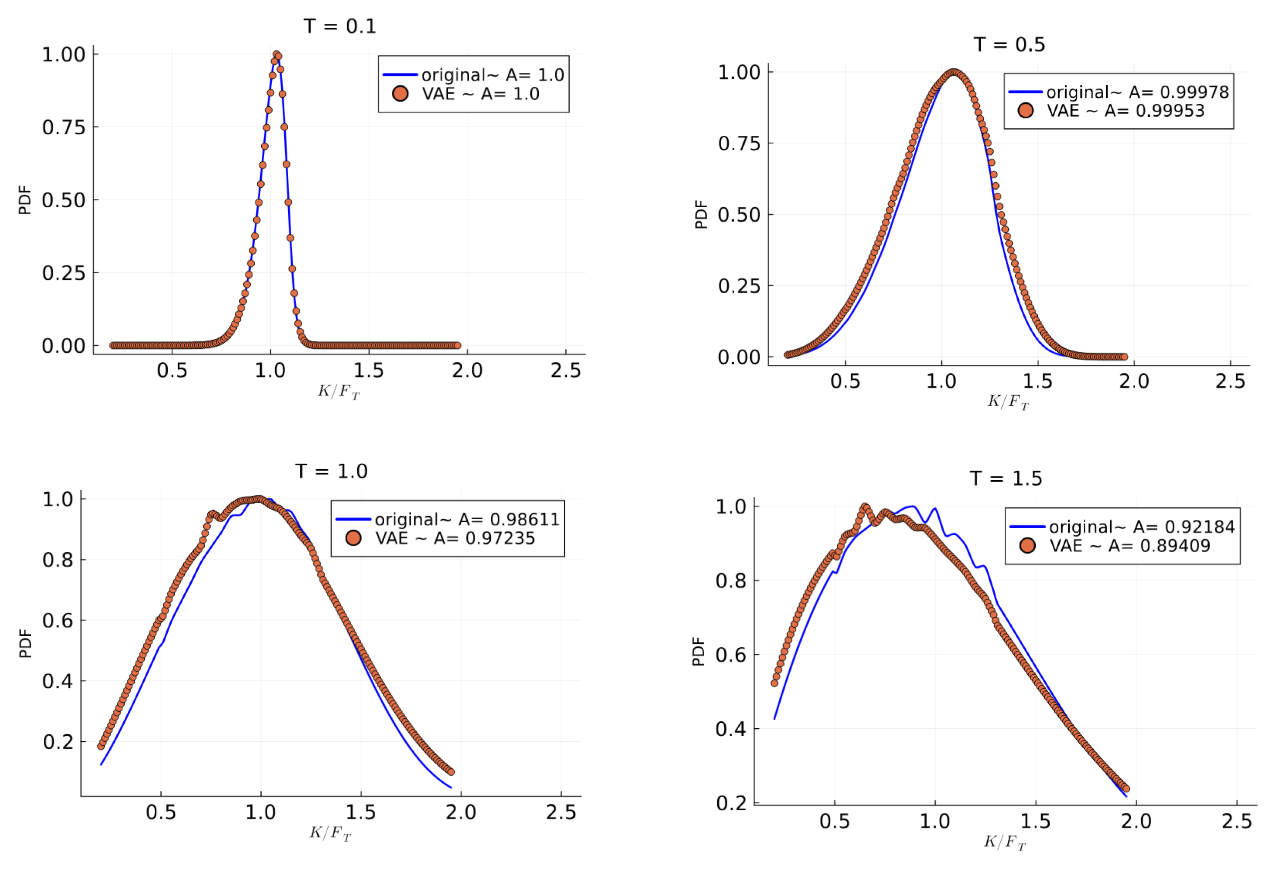
7.3.1. Butterfly Arbitrage Test

As explained in Section 4.2, butterfly arbitrage is evaluated by examining the risk-neutral density implied by the volatility surface. Figure 10 shows the probability density functions derived from both original and reconstructed surfaces at different maturities.

The results confirm the following:

• The density functions remain strictly positive across all strikes.
• The reconstructed densities closely match the original distributions.
• The area under each curve approximates 1, as required for a valid probability distribution.

These findings demonstrate that our approach successfully preserves the butterfly arbitrage-free property, even when reconstructing from sparse data.

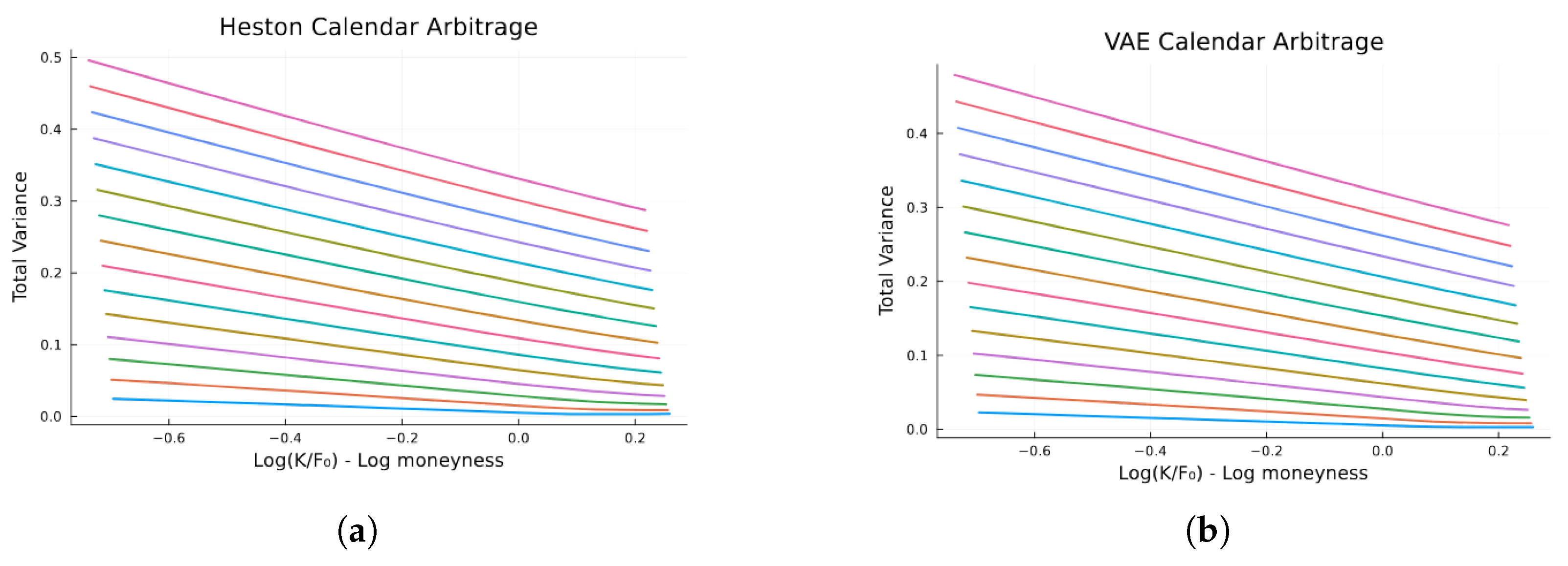
7.3.2. Calendar Spread Arbitrage Test

The calendar spread arbitrage condition requires that total variance (${\sigma }^{2}T$) increases monotonically with maturity for each strike. Figure 11 compares the total variance plots for both original Heston and VAE-reconstructed surfaces.

The non-intersection of these curves confirms that our approach maintains the calendar spread arbitrage-free property. The total variance increases monotonically with maturity across all strikes, preserving the essential structure required for legitimate financial modeling.

7.4. Comparison with Baseline Methods

To establish the effectiveness of our VAE approach with latent space optimization, we compare it against the baseline methods described in Section 5.4.

Table 4. Comparison of methods for volatility surface completion (60.0% missing data).

Method	MSE	RMSE	MAE	MAPE (%)	Max Error
Variational Autoencoder (Ours)	4.39 × 10−6	0.00209	0.00171	0.81	0.00637
Thin-Plate Spline	8.76 × 10−6	0.00296	0.00242	1.17	0.01253
Deterministic Autoencoder	7.21 × 10−6	0.00269	0.00218	1.04	0.00896
SABR Model	1.52 × 10−5	0.00390	0.00332	1.59	0.01487
SVI Parameterization	1.28 × 10−5	0.00358	0.00301	1.42	0.01325

presents the results for the 60% missing data scenario.

Our VAE approach with latent space optimization consistently outperforms all baseline methods across all metrics. The performance advantage is particularly notable in comparison to traditional parametric approaches (SABR and SVI), which show errors 3–4 times higher than our method.

The deterministic autoencoder, which uses an identical architecture but lacks the variational component, performs significantly worse than our VAE approach. This confirms the importance of the probabilistic latent space representation for capturing the underlying structure of volatility surfaces.

This analysis reveals a key advantage of our method: it combines the flexibility of machine learning approaches with near-parametric quality in maintaining theoretical constraints. This balance is particularly valuable in financial applications where both accuracy and theoretical consistency are essential.

Table 5. Comparison across different sparsity levels (MSE × 10⁻⁶).

Method	20% Missing	40% Missing	60% Missing	80% Missing	96% Missing
Variational Autoencoder (Ours)	3.71	3.91	4.39	5.40	5.21
Thin-Plate Spline	4.25	6.19	8.76	15.42	37.63
Deterministic Autoencoder	5.13	6.28	7.21	9.47	19.85
SABR Model	6.89	10.26	15.20	26.78	64.31
SVI Parameterization	6.12	8.74	12.80	22.14	53.76

examines performance across different sparsity levels. While all methods show degrading performance with increasing sparsity, our VAE approach demonstrates remarkable resilience. At 96% missing data, our method maintains an MSE approximately 7–12 times lower than competing approaches, highlighting its effectiveness in extreme data-sparse scenarios.

These comparative results demonstrate that our VAE approach with latent space optimization represents a significant advancement in volatility surface modeling, particularly for incomplete data scenarios.

8. Conclusions and Implications

Our research has demonstrated the effectiveness of variational autoencoders (VAEs) for completing volatility surfaces while preserving essential arbitrage-free properties. In this concluding section, we synthesize our findings, discuss their implications for financial practice, acknowledge limitations, and suggest directions for future research.

8.1. Summary of Key Findings

Our investigation has produced several significant findings that advance the state of the art in volatility surface modeling. Our VAE framework successfully reconstructs volatility surfaces with remarkable accuracy, achieving mean squared errors below 4 × 10⁻⁶ on complete surfaces and maintaining low errors even with substantial missing data. This performance validates hypothesis H1, confirming that deep generative models can effectively capture the complex structure of volatility surfaces. Furthermore, the latent space optimization approach consistently outperforms standard reconstruction across all sparsity levels, with the performance gap widening as the percentage of missing data increases. With 96% missing data, latent optimization reduces error by 73.3% compared to standard reconstruction on the training set, supporting hypothesis H2. Our model also demonstrates the ability to reconstruct high-quality volatility surfaces with up to 96% missing data points (retaining only 12 of 255 grid points), achieving errors of approximately 5.2 × 10⁻⁶ on the training set and 3.62 × 10⁻⁶ on the validation set. These results confirm hypothesis H4 regarding reconstruction capability under extreme sparsity conditions. Finally, our approach consistently outperforms established baseline methods including thin-plate spline interpolation, deterministic autoencoders, SABR model, and SVI parameterization. This advantage becomes particularly pronounced in high-sparsity scenarios, where our method maintains 7–12 times lower error rates than competing approaches. These findings demonstrate that VAEs, when enhanced with latent space optimization, provide a powerful framework for volatility surface completion that balances statistical accuracy with financial relevance.

8.2. Theoretical and Practical Implications

Our research contributes to both the theoretical understanding of machine learning applications in finance and practical tools for market participants. Our framework demonstrates a successful integration of financial theory with modern machine learning techniques, showing that domain-specific constraints can be effectively incorporated into deep learning models. This addresses concerns about “black box” approaches in financial applications. The synthetic data generation approach leverages structured priors (Heston model dynamics) to enable data-efficient learning, suggesting a broader paradigm for financial modeling where theoretical models and machine learning techniques complement, rather than compete with, each other. On the practical side, the ability to rapidly and accurately complete volatility surfaces can improve market making in options markets, particularly for less liquid strikes and maturities. This could potentially reduce bid–ask spreads and increase market efficiency. Additionally, our approach enables more comprehensive risk analysis by providing complete volatility surfaces for scenario testing, VaR calculations, and stress testing, even in markets with limited liquidity or data availability. The robust performance under extreme sparsity makes our approach particularly valuable for emerging markets or newly introduced derivatives where limited trading activity results in highly incomplete volatility surfaces.

8.3. Limitations and Future Research Directions

Despite the promising results, our study has several limitations that should be acknowledged. While our use of synthetic data enabled comprehensive testing across diverse scenarios, real market data may exhibit features not captured by the Heston model. Future work should incorporate extensive testing on actual market data. Our implementation also assumes a fixed grid of strikes and maturities, whereas real markets have irregular strike/maturity combinations that may require additional preprocessing or model adaptations. Furthermore, our study focused on equity index-like volatility surfaces, but different asset classes (e.g., FX, commodities, interest rates) may exhibit different volatility dynamics requiring specialized adaptations.

These limitations suggest several promising directions for future research. Extending the VAE framework to jointly model volatility surfaces across multiple assets could potentially capture cross-asset relationships and correlations. Incorporating temporal evolution of volatility surfaces by integrating recurrent neural network components or utilizing spatiotemporal extensions of VAEs would add another valuable dimension to the model. Developing hybrid approaches that combine the strengths of parametric models (interpretability, theoretical consistency) with the flexibility and accuracy of deep learning methods represents another promising avenue. Finally, directly modeling the implied risk-neutral probability distributions rather than volatility surfaces might offer more direct arbitrage enforcement.

8.4. Concluding Remarks

The integration of deep generative modeling with financial mathematics represents a significant advancement in volatility surface modeling. Our research demonstrates that variational autoencoders, enhanced with latent space optimization, provide a powerful framework for completing volatility surfaces from sparse data while maintaining essential arbitrage-free properties. By bridging machine learning capabilities with financial theory constraints, our approach offers both theoretical insights and practical tools for market participants. The ability to generate complete, arbitrage-free volatility surfaces from minimal data points has far-reaching implications for pricing, risk management, and trading strategies, particularly in markets characterized by limited liquidity or data availability. As financial markets continue to evolve and generate increasingly complex derivative instruments, the need for sophisticated modeling approaches will only grow. We believe that deep generative models, with their ability to capture complex distributions while respecting theoretical constraints, will play an increasingly important role in the future of quantitative finance.

References

- Andersen, L., & Andreasen, J. (2000). Jump-diffusion processes: Volatility smile fitting and numerical methods for option pricing. Review of Derivatives Research, 4(3), 231–262. [Google Scholar] [CrossRef]
- Bates, D. S. (1996). Jumps and stochastic volatility: Exchange rate processes implicit in Deutsche Mark options. Review of Financial Studies, 9(1), 69–107. [Google Scholar] [CrossRef]
- Bergeron, M., Fung, N., Hull, J., & Poulos, Z. (2021). Variational autoencoders: A hands-off approach to volatility. arXiv, arXiv:2102.03945. [Google Scholar] [CrossRef]
- Black, F., & Scholes, M. (1973). The pricing of options and corporate liabilities. Journal of Political Economy, 81(3), 637–654. [Google Scholar] [CrossRef]
- Cao, J., Li, J., & Tu, X. (2020). Yield curve modeling using variational autoencoders. Journal of Risk and Financial Management, 13(12), 322. [Google Scholar]
- Christoffersen, P., Heston, S., & Jacobs, K. (2009). The shape and term structure of the index option smirk: Why multifactor stochastic volatility models work so well. Management Science, 55(12), 1914–1932. [Google Scholar] [CrossRef]
- Cont, R., & Vuletić, M. (2023). Simulation of arbitrage-free implied volatility surfaces. Applied Mathematical Finance, 30(2), 94–121. [Google Scholar] [CrossRef]
- Dumas, B., Fleming, J., & Whaley, R. E. (1998). Implied volatility functions: Empirical tests. Journal of Finance, 53(6), 2059–2106. [Google Scholar] [CrossRef]
- Dupire, B. (1994). Pricing with a smile. Risk, 7(1), 18–20. [Google Scholar]
- Fengler, M. R. (2009). Arbitrage-free smoothing of the implied volatility surface. Quantitative Finance, 9(4), 417–428. [Google Scholar] [CrossRef]
- Ferguson, R., & Green, A. (2018). Deeply learning derivatives. arXiv, arXiv:1809.02233. [Google Scholar]
- Gatheral, J. (2004). A parsimonious arbitrage-free implied volatility parameterization with application to the valuation of volatility derivatives. Global Derivatives & Risk Management. Available online: https://api.semanticscholar.org/CorpusID:156076635 (accessed on 14 February 2025).
- Gatheral, J. (2006). The volatility surface: A practitioner’s guide. Wiley Finance. [Google Scholar]
- Gatheral, J., Jusselin, P., & Rosenbaum, M. (2020). The quadratic rough Heston model and the joint S&P 500/VIX smile calibration problem. Quantitative Finance, 20(10), 1593–1608. [Google Scholar]
- Goodfellow Ian, J., Pouget-Abadie, J., Mirza, M., Xu, B., Warde-Farley, D., Ozair, S., Courville, A., & Bengio, Y. (2014). Generative adversarial nets. Available online: https://arxiv.org/abs/1406.2661v1 (accessed on 14 February 2025).
- Hagan, P., Kumary, D. M., LESNIEWSKIz, A. S., & WOODWARDx, D. E. (2002). Managing smile risk. Available online: https://api.semanticscholar.org/CorpusID:220747493 (accessed on 14 February 2025).
- Heston, S. L. (1993). A closed-form solution for options with stochastic volatility with applications to bond and currency options. The Review of Financial Studies, 6(2), 327–343. [Google Scholar] [CrossRef]
- Hinton, G. E., & Salakhutdinov, R. R. (2006). Reducing the dimensionality of data with neural networks. Science, 313(5786), 504–507. [Google Scholar] [CrossRef] [PubMed]
- Horvath, B., Muguruza, A., & Tomas, M. (2021). Deep learning volatility: A deep neural network perspective on pricing and calibration in (rough) volatility models. Quantitative Finance, 21(1), 11–27. [Google Scholar] [CrossRef]
- Hutchinson, J. M., Lo, A. W., & Poggio, T. (1994). A nonparametric approach to pricing and hedging derivative securities via learning networks. Journal of Finance, 49(3), 851–889. [Google Scholar] [CrossRef]
- Kingma, D. P., & Welling, M. (2013). Auto-encoding variational Bayes. arXiv, arXiv:1312.6114. [Google Scholar]
- Kondratyev, A., & Schwarz, C. (2019). The market generator. SSRN Electronic Journal. [Google Scholar] [CrossRef]
- Liu, S., Oosterlee, C. W., & Bohte, S. M. (2019). Pricing options and computing implied volatilities using neural networks. Risks, 7(1), 16. [Google Scholar] [CrossRef]
- McGhee, W. A. (2018). An artificial neural network representation of the SABR stochastic volatility model. SSRN Electronic Journal, Journal of Computational Finance. Available online: https://papers.ssrn.com/sol3/papers.cfm?abstract_id=3288882 (accessed on 14 February 2025).
- Takahashi, S., Chen, Y., & Tanaka-Ishii, K. (2019). Modeling financial time-series with generative adversarial networks. Physica A: Statistical Mechanics and Its Applications, 527, 121261. [Google Scholar] [CrossRef]
- Wahba, G. (1990). Spline models for observational data. CBMS-NSF Regional Conference Series in Applied Mathematics, Series Number 59. Society for Industrial and Applied Mathematics (SIAM). [Google Scholar] [CrossRef]
- Wiese, M., Knobloch, R., Korn, R., & Kretschmer, P. (2019). Quant GANs: Deep generation of financial time series. Quantitative Finance, 20(9), 1419–1440. [Google Scholar] [CrossRef]