Article

Impact of the COVID-19 Pandemic on the Financial Market Efficiency of Price Returns, Absolute Returns, and Volatility Increment: Evidence from Stock and Cryptocurrency Markets

Department of Liberal Arts, Hiroshima University of Economics, Hiroshima 731-0192, Japan
J. Risk Financial Manag. 2025, 18(5), 237; https://doi.org/10.3390/jrfm18050237
Submission received: 2 April 2025 / Revised: 23 April 2025 / Accepted: 25 April 2025 / Published: 29 April 2025

Abstract

:
This study examines the impact of the coronavirus disease 2019 (COVID-19) pandemic on market efficiency by analyzing three time series—price returns, absolute returns, and volatility increments—in the stock (Deutscher Aktienindex, Nikkei 225, Shanghai Stock Exchange (SSE), and Volatility Index) and cryptocurrency (Bitcoin and Ethereum) markets. The effect is found to vary by asset class and market. In the stock market, while the pandemic did not influence the Hurst exponent of volatility increments, it affected that of returns and absolute returns (except in the SSE, where returns remained unaffected). In the cryptocurrency market, the pandemic did not alter the Hurst exponent for any time series but influenced the strength of multifractality in returns and absolute returns. Some Hurst exponent time series exhibited a gradual decline over time, complicating the assessment of pandemic-related effects. Consequently, segmented analyses by pandemic period may erroneously suggest an impact, warranting caution in period-based studies.

1. Introduction

Fama (1970) developed and classified the efficient market hypothesis (EMH) into three forms: (i) weak, (ii) semi-strong, and (iii) strong. The weak-form efficient market considers only historical prices, asserting that current prices include all past information, making future prices unpredictable. Weak-form efficient markets have been extensively tested. To date, no definitive answer has been obtained. Rather, the possibility that the market efficiency may change over time was discussed in (Lim & Brooks, 2011).
One statistical model that can match this market is the random walk model. Therefore, numerous studies have attempted to determine whether time series exhibit randomness. A popular method when testing the randomness of a time series is to measure the Hurst exponent h of the time series, introduced by (Hurst, 1951). For a random time series, h = 0.5 . Thus, h 0.5 is used as an indicator of market inefficiency. For a time series with h > 0.5 , successive movements in the same direction were observed more often than in the random walk process. A time series with h > 0.5 is denoted as “persistent”. Conversely, time series with h < 0.5 have successive movement back and forth more often than the random walk process, denoted as “anti-persistent”.
Matteo et al. (2005) investigated the Hurst exponents of 32 world stock market indices and classified them based on their Hurst exponents. They found that, while all emerging markets belong to a group with h > 0.5 (persistent), developed markets fall into groups with either h = 0.5 (random) or h < 0.5 (anti-persistent). Well-developed markets (the USA, Japan, France, and Australia) are classified as follows: a group with h < 0.5 , which indicates inefficiency. Takaishi (2022b) investigated the time evolution of the Hurst exponent for the Japanese stock market and found that, in the early stage of the market, the Hurst exponent was higher than 0.5; it then gradually decreased and dropped below 0.5 around the year 2000, indicating anti-persistency. The Bitcoin market at the early stage also showed anti-persistency for return time series (Takaishi, 2018; Urquhart, 2016). This anti-persistency gradually disappeared as the Bitcoin market matured (Drożdż et al., 2018). The anti-persistency observed in the early stage of the Bitcoin market was linked to the poor liquidity of the market (Takaishi & Adachi, 2020; Wei, 2018).
Another anti-persistent time series is found in the volatility increment time series, which is an important property in modeling and forecasting volatility. Gatheral et al. (2018) investigated the Hurst exponent of the realized volatility time series and found that the realized volatility time series exhibited anti-persistency, denoted as “rough volatility”. This property has been further confirmed through subsequent studies on various assets and implied volatility (Bennedsen et al., 2022; Brandi & Di Matteo, 2022; Floc’h, 2022; Livieri et al., 2018; Takaishi, 2020). Takaishi (2022a) investigated the Hurst exponent of trading volume increment time series and showed that the trading volume increment time series was anti-persistent, and the time variation of the Hurst exponent was closely related to that of the volatility increment time series.
The coronavirus disease 2019 (COVID-19) pandemic, officially declared a pandemic by World Health Organization (WHO) on 11 March 2020, significantly affected the global economy. Financial markets were also heavily disrupted by COVID-19, suggesting that market efficiency was affected. The impact of COVID-19 on market efficiency has been studied across various financial asset time series. The results indicate that, in many cases, market efficiency deteriorated due to the impact of COVID-19 (see, e.g., Alijani et al. (2021); Aslam et al. (2020a); Aslam et al. (2020b); Erer et al. (2023); Fernandes et al. (2022); Mensi et al. (2021, 2020); Raza et al. (2024); Shen and Chen (2022); J. Wang et al. (2020); Zitis et al. (2023)).
However, COVID-19 seems to have affected financial assets differently. Saâdaoui (2023) analyzed the impact of COVID-19 on stock market indices and found that, while the multifractality for the USA, Japanese, and Eurozone markets increased after the pandemic, the Chinese market’s multifractality decreased. Ameer et al. (2023) examined the responses of the Brazil, Russia, India, China, and South Africa (BRICS) and Morgan Stanley Capital International (MSCI) emerging stock market indices to the COVID-19 pandemic and found that COVID-19 increased the market inefficiency, except in China. They concluded that China’s market efficiency improved after the COVID-19 outbreak.
Mnif et al. (2020) studied the cryptocurrency efficiency and found that COVID-19 has positively impacted the cryptocurrency market, and cryptocurrencies have become more efficient since the pandemic. J. Wang and Wang (2021) examined market efficiency using entropy-based analysis for S&P 500, gold, Bitcoin, and the US dollar index and found that, while these market efficiencies decreased because of COVID-19, the Bitcoin market efficiency was more resilient than the others. Diniz-Maganini et al. (2021) also claimed that the Bitcoin prices are more efficient than the US dollar and MSCI world indices. Conversely, Naeem et al. (2021) showed that the COVID-19 outbreak adversely affected the efficiency of four cryptocurrencies (Bitocoin, Ethereum, Litecoin, and Ripple) given the substantial increases in the levels of inefficiency during the COVID-19 period.
Most previous studies have utilized price return data for multifractal analysis; however, some studies have examined the impact of COVID-19 using other types of time series data. For example, using a wavelet-based method, Arouxet et al. (2022) estimated the Hurst exponent of a volatility time series and detected a temporary impact on volatility during the peak of the COVID-19 pandemic. Lahmiri (2023) investigated multifractality for both price returns and trading volume variation time series of cryptocurrencies and found that the multifractality decreased during the pandemic for both time series.
We investigate the time evolution of market efficiency and examine the impact of the COVID-19 pandemic on the time variation in market efficiency. We analyze three types of time series—namely, returns, absolute returns, and volatility increments—in order to clarify the effects of the COVID-19 pandemic on these time series. To the best of our knowledge, this study is the first to examine the impact of the COVID-19 pandemic on volatility increments. Recent research on volatility has shown that volatility increment time series provide crucial information for the modeling of volatility. After Gatheral et al. (2018) demonstrated the roughness of volatility increment time series, the modeling of volatility using models with roughness became increasingly popular. Several advantages of models with roughness based on fractional Brownian motion are also known. For example, it has been pointed out that models with roughness can explain the negative power law of implied volatility (Alos et al., 2007; Fukasawa, 2011). It has also been suggested that rough models could serve as a theoretical framework to explain the time-reversal asymmetry observed in the correlation between realized volatility and returns—a phenomenon commonly known as the Zumbach effect (Zumbach, 2003, 2009). Consequently, analyzing various types of time series, including volatility increment time series, is expected to provide comprehensive insights into the pandemic’s impact on individual markets.
We quantify market efficiency using the generalized Hurst exponent (GHE) obtained via multifractal detrended fluctuation analysis (MFDFA) (Kantelhardt et al., 2002) and examine the effect of the COVID-19 pandemic on the stock and cryptocurrency markets according to the time evolution of market efficiency.
The remainder of this paper is organized as follows. Section 2 describes the data used in this study. Section 3 describes the proposed methodology. Section 4 presents our results. Finally, Section 5 presents the discussion and conclusions.

2. Data

We retrieved the daily closing prices P ( t ) of the four indices (DAX, Nikkei 225, SSE, and VIX) from https://finance.yahoo.com (accessed on 25 January 2024). These time series data cover the period from 3 July 1997 to 19 January 2024, including the time of the financial crisis initiated by Lehman and the COVID-19 pandemic. We also obtained the daily closing prices P ( t ) of cryptocurrencies (Bitcoin and Ethereum) from https://www.investing.com (accessed on 10 January 2025). The data collection period was from 11 March 2016 to 31 December 2024, which included the COVID-19 pandemic period only.
The return r ( t ) is defined as the logarithmic price difference as follows:
r ( t ) = log P ( t ) log P ( t 1 ) .
We use the absolute return A R ( t ) | r ( t ) | as a proxy for volatility, with a long memory property (Ding et al., 1993). We also define the volatility increment V I ( t ) using the absolute return A R ( t ) as follows:
V I ( t ) = log A R ( t ) log A R ( t 1 ) .
Figure 1 illustrates the return, absolute return, and volatility increment time series of Bitcoin.
Table 1 summarizes the descriptive statistics of the time series. The means of most time series for the return and volatility increments are consistent with zero within a one-sigma error. The kurtosis values of the volatility increment are slightly higher than those of the Gaussian distribution, similar to those obtained for realized volatility increments (Takaishi, 2020).

3. Methodology

3.1. MFDFA

To examine the multifractal properties of a time series, we use MFDFA Kantelhardt et al. (2002). MFDFA is described using the following steps.
(i) We determine the profile Y ( i ) ,
Y ( i ) = j = 1 i ( r ( j ) r ) ,
where r denotes the average.
(ii) We divide profile Y ( i ) into N s non-overlapping segments of equal length s, where N s i n t ( N / s ) . A short period may exist at the end of the profile because the length of the time series is not always a multiple of s. To utilize this part, the same procedure is repeated, starting from the end of the profile. Thus, 2 N s segments are obtained.
(iii) We calculate the variance
F 2 ( ν , s ) = 1 s i = 1 s ( Y [ ( ν 1 ) s + i ] P ν ( i ) ) 2 ,
for each segment, ν , ν = 1 , , N s and
F 2 ( ν , s ) = 1 s i = 1 s ( Y [ N ( ν N s ) s + i ] P ν ( i ) ) 2 ,
for each segment, ν , ν = N s + 1 , , 2 N s , where P ν ( i ) is the fitting polynomial used to remove the local trend in segment ν .
P ν ( i ) = k = 0 p a k i k .
Here, we use a cubic-order ( p = 3 ) polynomial.
(iv) We average over all segments and obtain the qth-order fluctuation function:
F q ( s ) = 1 2 N s ν = 1 2 N s ( F 2 ( ν , s ) ) q / 2 1 / q .
(v) We determine the GHE h ( q ) from the scaling exponent of F q ( s ) . If the time series r ( i ) is long-range power-law correlated, F q ( s ) is expected to have the following functional form for a large s:
F q ( s ) s h ( q ) .
The singularity spectrum f ( α ) , which also characterizes the multifractality of the time series, is defined by h ( q ) as
f ( α ) = q [ α h ( q ) ] + 1 ,
where α is the Hölder exponent or singularity strength, given by
α = h ( q ) + q h ( q ) .
The Hurst exponent is obtained using h ( 2 ) . We restrict the range of q to q = [ 5 , 5 ] because, when | q | is large, the moments in the fluctuation function diverge, and the calculation of h ( q ) may be unstable (Jiang et al., 2019).
We define the strength of multifractality by the width of h ( q ) as (Zunino et al., 2008)
Δ h ( q ) = h ( q ) h ( q ) ,
where q 0 . Since a Gaussian time series exhibits a monofractal nature with Δ h ( q ) = 0 , a nonzero Δ h ( q ) suggests that the strength of multifractality is associated with the degree of market inefficiency. Similarly, the strength of multifractality can be defined by the width of the singularity spectrum α ( q ) as follows:
Δ α ( q ) = α ( q ) α ( q ) .
Δ α ( q ) is zero for the monofractal time series.

3.2. Market Efficiency Measurement by GHE

Since the Hurst exponent h ( 2 ) of a random time series is 0.5, any deviation from this value suggests inefficiencies in the time series. Y. Wang et al. (2009) proposed the market deficiency measure (MDM), defined by an average deviation from 0.5 as
M D M ( q ) = 1 2 ( | h ( q ) 0.5 | + | 0.5 h ( q ) | ) ,
which is zero in efficient markets. We observe that M D M ( q ) reduces Δ h ( q ) , disregarding a prefactor, for the conditions h ( q ) 0.5 > 0 and 0.5 h ( q ) > 0 , which are typically satisfied. Thus, the multifractal strength Δ h ( q ) is also related to inefficiencies quantified by deviations from 0.5.

4. Empirical Results

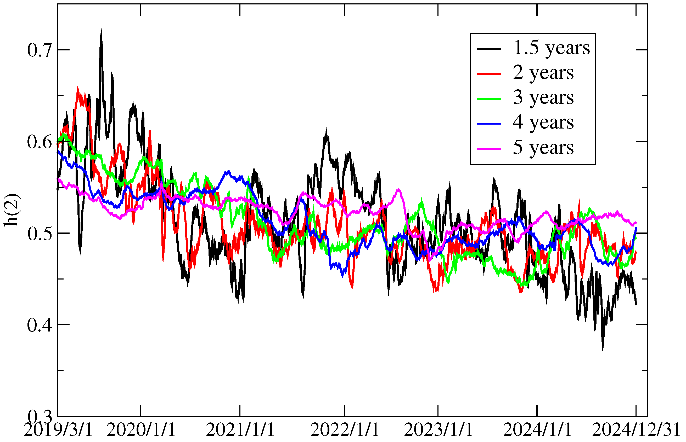
To obtain the temporal evolution of h ( q ) , we employed the rolling window method and selected an appropriate window size. While smaller window sizes are preferred for better time resolution, statistical fluctuations increase as the window (data) size decreases. Figure 2 illustrates the time evolution of h ( 2 ) for Bitcoin returns, computed using window sizes of 1.5, 2, 3, 4, and 5 years with a rolling window that shifts by one day at a time. We observe that all time evolution patterns exhibit similar trends; however, larger fluctuations are evident with smaller window sizes. Consequently, we selected a 3-year rolling window (1095 days) that demonstrated acceptable fluctuations. As trading does not occur in the stock market daily, we selected 750 working days as the approximately 3-year period for the time series data in the stock market.
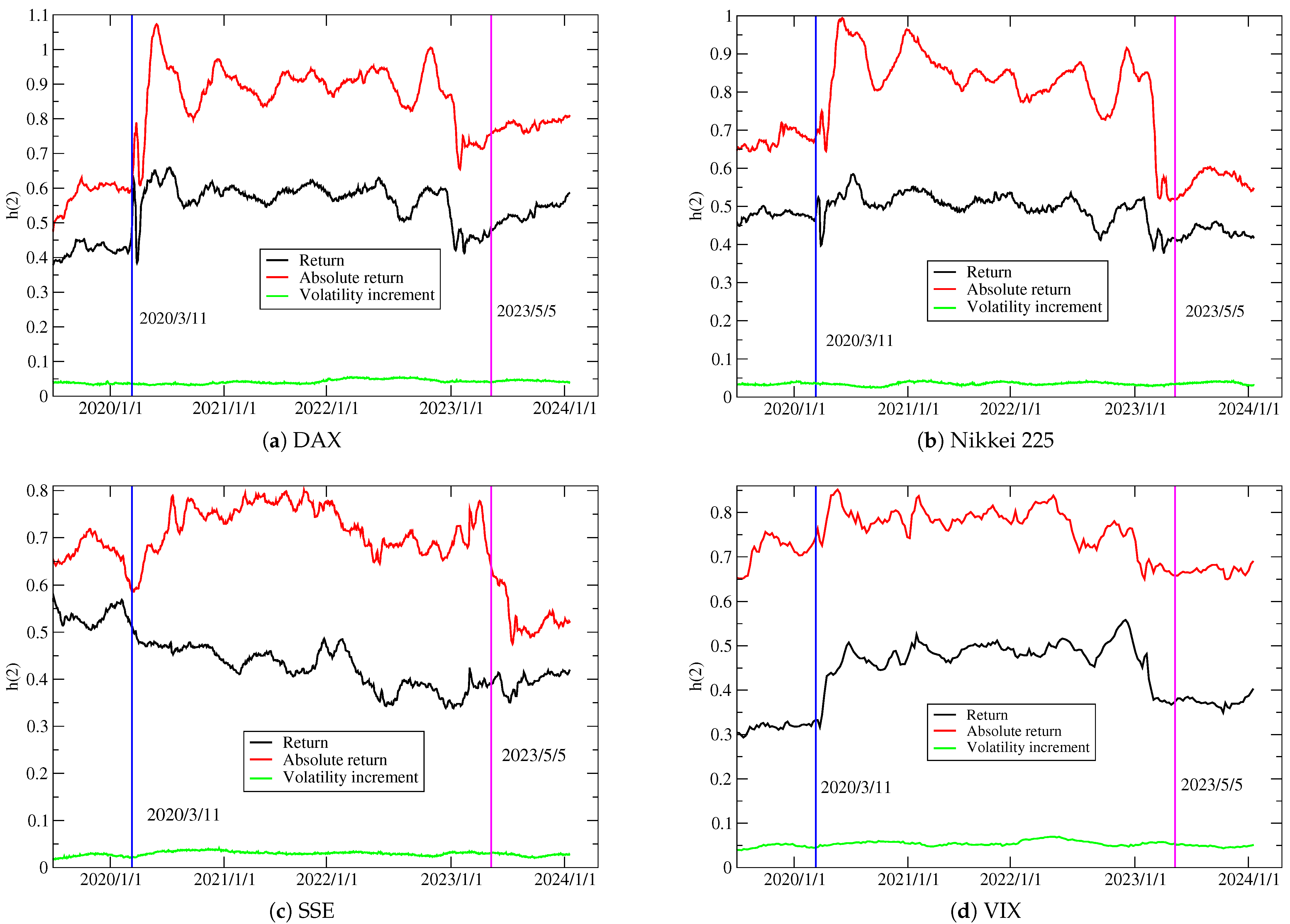
First, we show the time evolution of the Hurst exponent h ( 2 ) for DAX, Nikkei 225, SSE, and VIX in Figure 3 and provide an overview of the properties of the four time series. The Hurst exponents of the return time series remain approximately 0.5, except for VIX, for which h ( 2 ) is less than 0.5, exhibiting anti-persistence. However, the Hurst exponents of the absolute return time series are greater than 0.5, reflecting the long-memory property of the absolute return time series (Ding et al., 1993). The Hurst exponents of the volatility increment time series are small, typically less than 0.1, which implies that the time series are anti-persistent.
We then focus on the impact of the Lehman Brothers’ bankruptcy (the black lines in Figure 3). We find no clear response to the impact of the Lehman Brothers’ bankruptcy in the time evolution of h ( 2 ) , except in the case of DAX and Nikkei 225, where it increased promptly. No clear impact of the Lehman Brothers’ bankruptcy on other stocks and the results of returns and volatility increments was observed.
To examine the COVID-19 period in more detail, we plot the results within the period from 1 July 2019 to 19 January 2024 in Figure 4. We find that the pandemic had a definite impact on both returns and absolute returns. However, no impact of the pandemic was observed for the h ( 2 ) of the volatility increment. In the case of DAX and Nikkei 225, the h ( 2 ) of returns and absolute returns reacted sensitively to the WHO’s declaration of a pandemic on 11 March 2020. Around the day of the WHO declaration, we observe that h ( 2 ) increased abruptly; it then suddenly decreased and then increased again. During the pandemic, h ( 2 ) remained higher than before the pandemic. After the WHO’s declaration at the end of the pandemic, h ( 2 ) returned to its previous levels.
Regarding the SSE and VIX, we observed a reaction similar to that of DAX and Nikkei 225, i.e., the h ( 2 ) of the returns on VIX and the h ( 2 ) of the absolute returns on the SSE and VIX increased around the time of the pandemic declaration and returned to the previous levels after the declaration of the end of the pandemic. An exceptional case is h ( 2 ) for the returns of the SSE, which did not react to the pandemic.
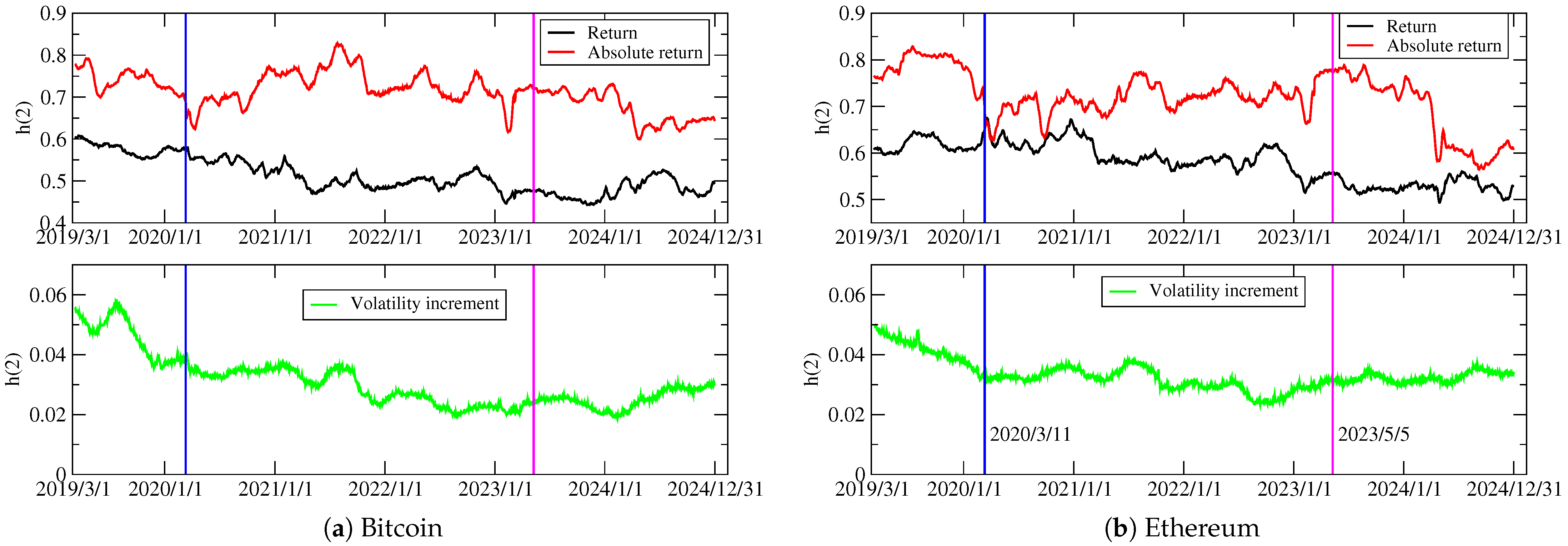
Figure 5 shows the results of h ( 2 ) for the cryptocurrencies Bitcoin and Ethereum. These results suggest that there was no discernible response to the pandemic. In contrast to the stock market, the h ( 2 ) of cryptocurrencies exhibits no reaction to the pandemic. Although the h ( 2 ) of returns for Bitcoin and Ethereum appeared to decrease gradually, we cannot conclude that this gradual decline is attributable to the pandemic. If we conduct a period-based analysis in this case, we might observe a pseudo-pandemic effect. For example, Table 2 shows the h ( 2 ) of returns for Bitcoin and Ethereum before and during the COVID-19 periods, indicating that, as the Hurst exponent gradually decreased, the market efficiency appeared to improve after the COVID-19 pandemic.
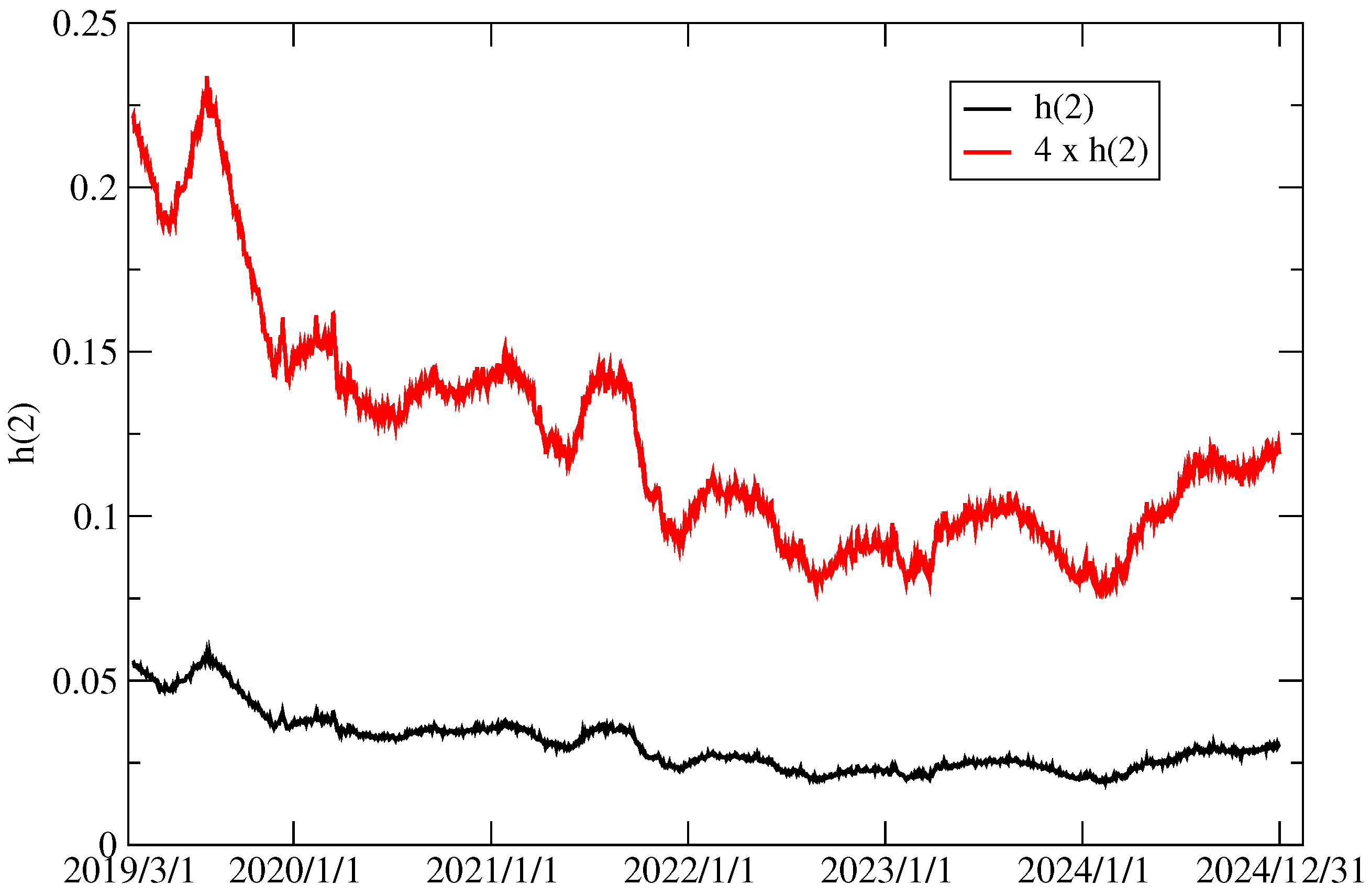
Similarly to the stock market, the h ( 2 ) of the volatility increment is low and exhibits anti-persistence. This anti-persistence is consistent with that observed for the realized and implied volatility time series, although the Hurst exponents of the volatility increment defined by absolute returns lead to a smaller Hurst exponent (Gatheral et al., 2018). For example, the Hurst exponent of Bitcoin’s realized volatility is calculated as approximately 0.12–14 (Takaishi, 2025). However, the Bitcoin volatility increment from absolute return volatility was approximately 0.02–0.04 in recent years, as shown in Figure 5, which is smaller than that of Bitcoin’s realized volatility. This reduction can be explained by the finite-sample effect on the realized volatility. Realized volatility is constructed using a finite sample of squared intraday returns (Andersen & Bollerslev, 1998; McAleer & Medeiros, 2008), and its accuracy depends on the sample size (Andersen et al., 2007; Fleming et al., 2003; Peters & De Vilder, 2006). Takaishi (2025) found that the Hurst exponent decreases as the sample size decreases, and they provide a phenomenological formula that describes the Hurst exponent as a function of the sample size:
H 2 ( n ) = H 2 n n + a 1 ,
where n is the sample size and a 1 is a fitting parameter. H 2 denotes the Hurst exponent at n . The absolute returns (or their square) correspond to the lowest-order realized volatility with n = 1 . Using a 1 3 obtained in Takaishi (2025) and n = 1 , we obtain
H 2 = H 2 ( 1 ) × 4 .
Figure 6 shows the Hurst exponent of Bitcoin’s volatility increment and its values multiplied by four. The results multiplied by four are close to the Hurst exponent obtained for Bitcoin’s realized volatility (0.12∼0.14), except for the results (∼0.2) around 2019.
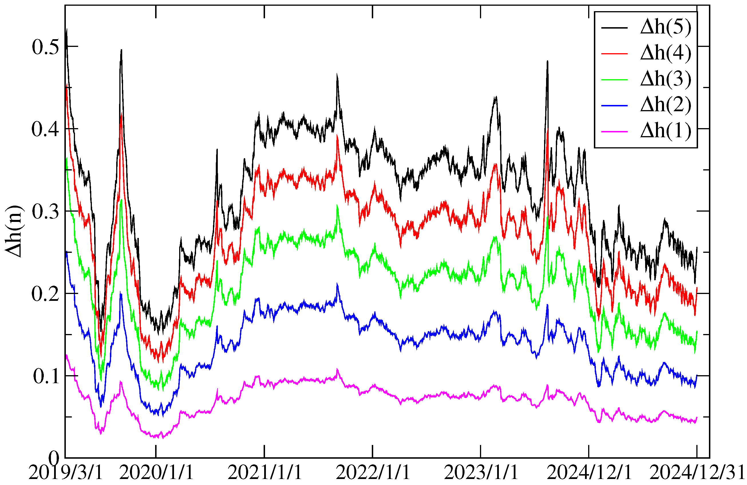
Finally, we analyzed the effect of the pandemic on the multifractal strength Δ h ( n ) . Although Δ h ( n ) depends on n, we observe that the temporal variation pattern exhibits similar fluctuations regardless of n, as illustrated in Figure 7. Consequently, by selecting n = 5 , we focus on Δ h ( 5 ) in the subsequent analysis.
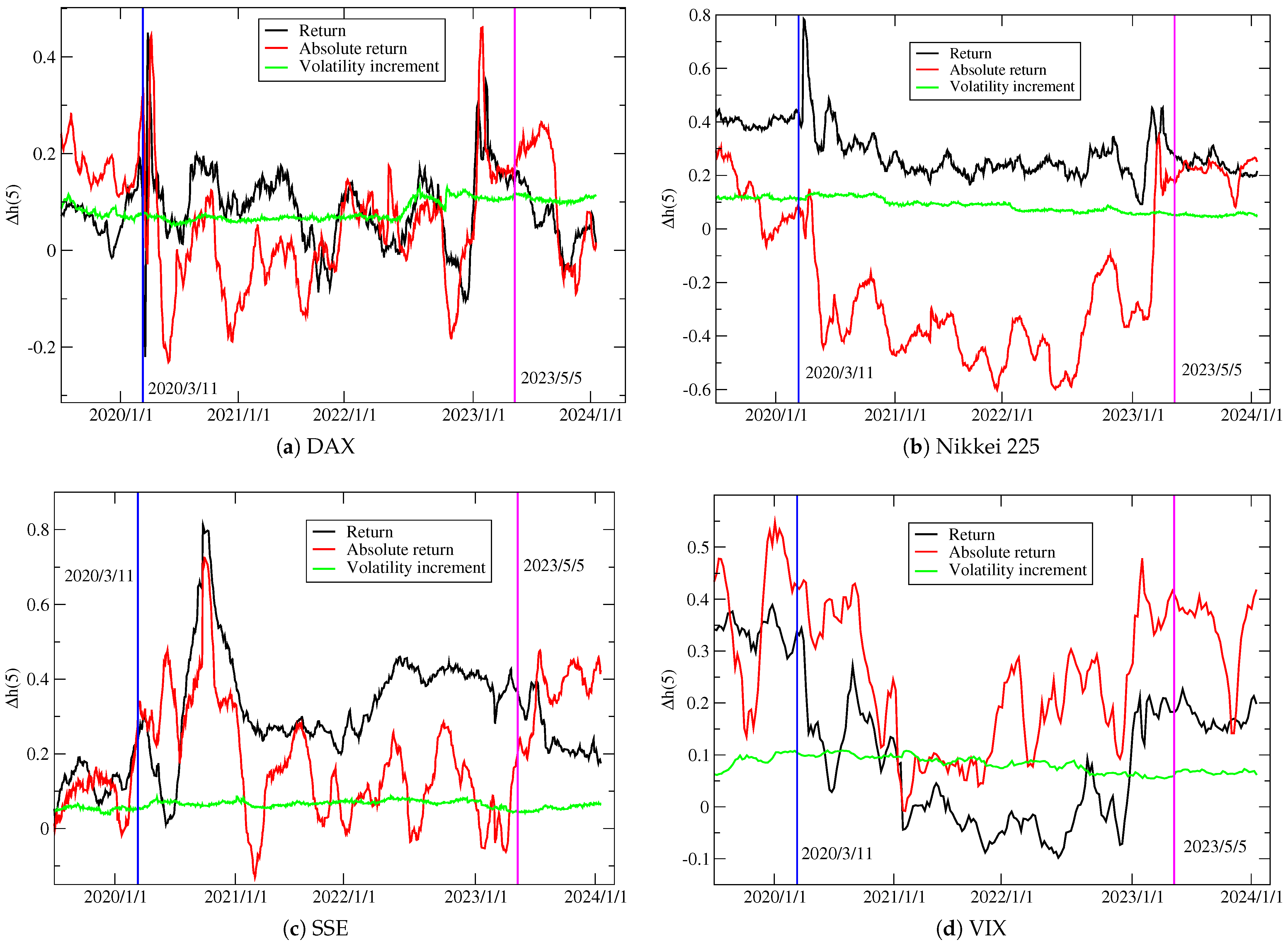
The stock market results of Δ h ( 5 ) are shown in Figure 8. We observe that the Δ h ( 5 ) of the volatility increment remained stable with positive values and did not respond to the pandemic. However, the Δ h ( 5 ) of the returns and absolute returns fluctuated dramatically, and negative values can be assumed. This observation implies that the functional form of h ( q ) changed significantly over time. Although the Δ h ( 5 ) of the returns and absolute returns for DAX and Nikkei 225 appeared to have responded to the pandemic, it is difficult to identify a pattern describing the impact of the pandemic.
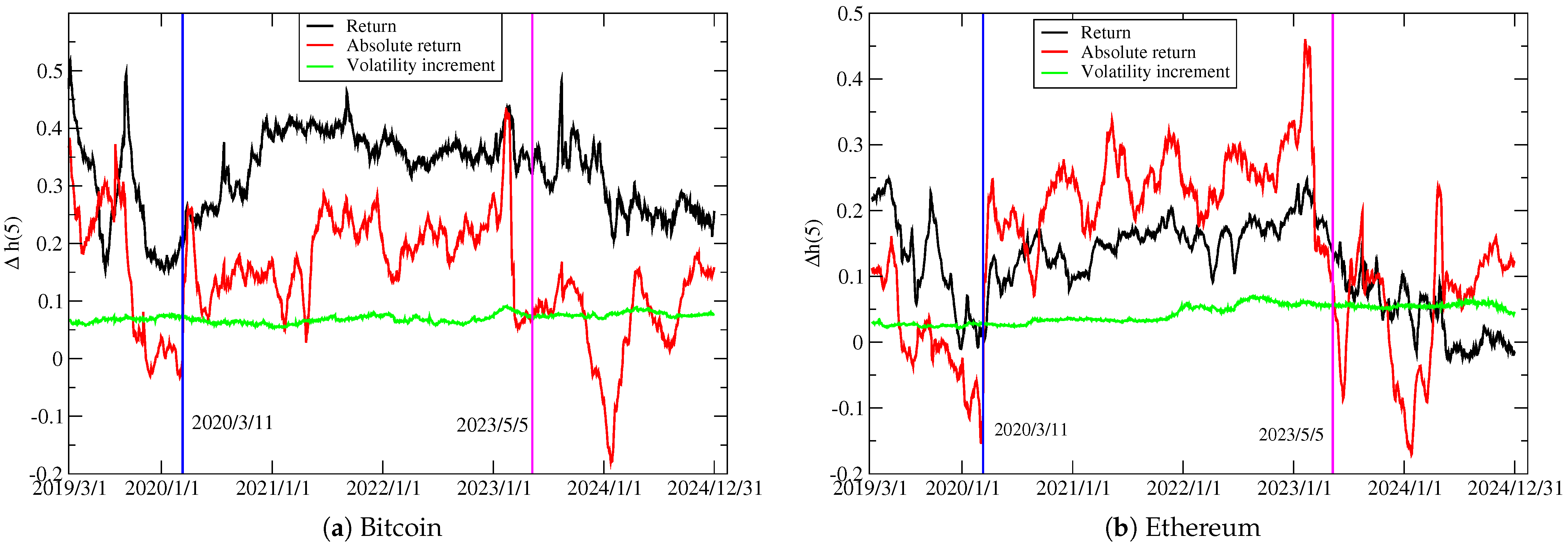
Figure 9 shows the time evolution of Δ h ( 5 ) for cryptocurrencies. Similarly to the stock market, the Δ h ( 5 ) of the volatility increment for cryptocurrencies remained stable with positive values. Although the Δ h ( 5 ) values of the returns and absolute returns fluctuate considerably, we identify a pattern in which Δ h ( 5 ) increased around the time of the pandemic declaration and obtained a smaller Δ h ( 5 ) value after the end of the COVID-19 pandemic.
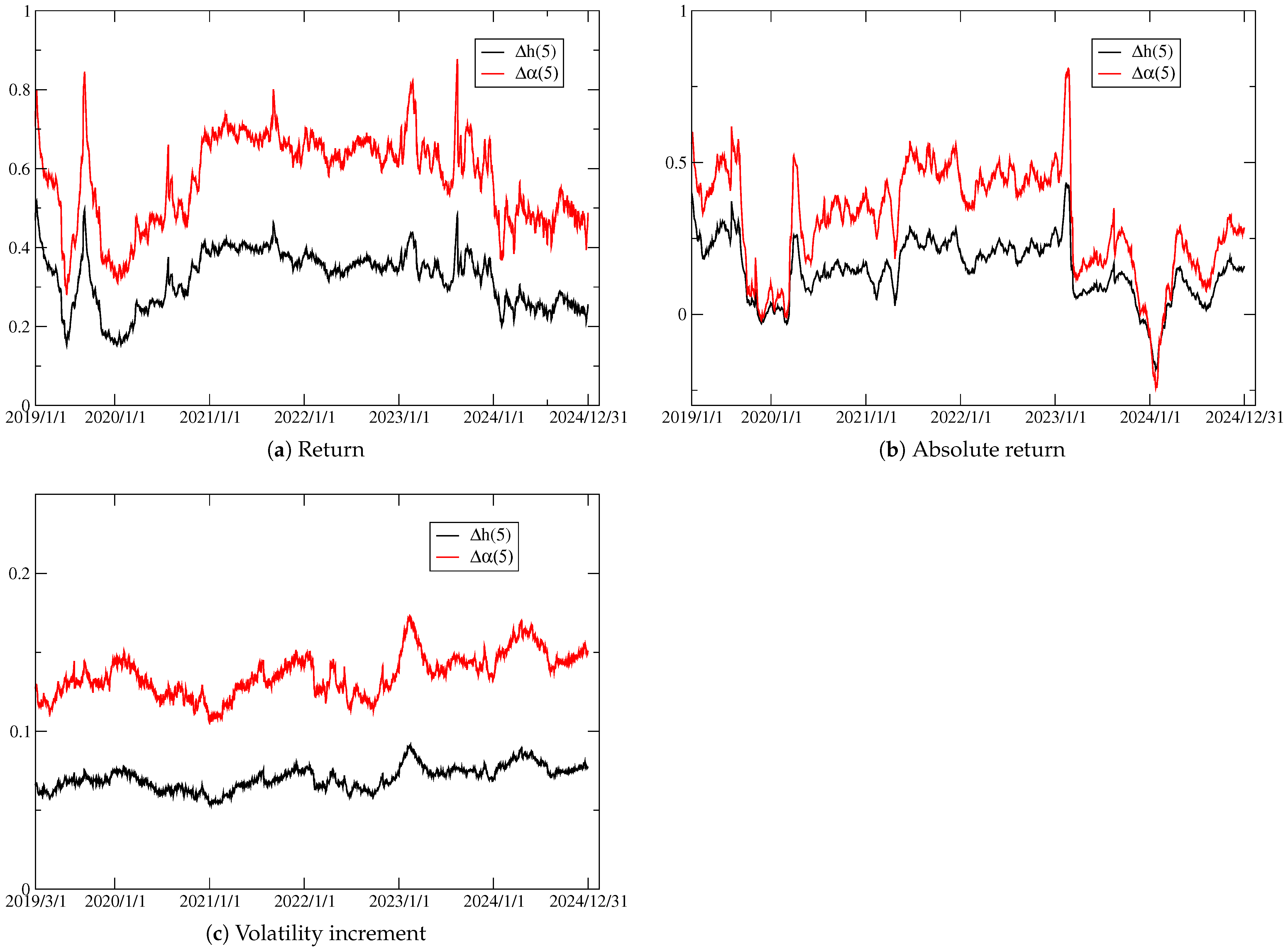
The multifractal strength is also defined by the singularity spectrum α ( q ) as in Equation (12). We compared Δ α ( 5 ) with Δ h ( 5 ) and discovered that both exhibited similar time variation patterns. For example, Figure 10 displays the time evolution of Δ α ( 5 ) and Δ h ( 5 ) for Bitcoin, demonstrating similar temporal patterns. Therefore, in such cases, the same conclusion can be drawn regarding the temporal variations. A comparison of Δ α ( q ) and Δ h ( q ) for Bitcoin returns is also provided in (Takaishi, 2021).
Table 3 summarizes whether the pandemic affected the time series. When the pandemic has an impact, its effect on efficiency is classified as “positive” if it leads to an improvement and “negative” if it has the opposite outcome. When an impact has been observed but improvements in efficiency are unclear, it is represented by the symbol ◯. The table indicates that the pandemic exerted varying impacts depending on the differences in the markets and types of time series. Broadly speaking, the COVID-19 pandemic affected all markets. However, a notable feature of the stock market is that the Hurst exponent of returns for the SSE shows no apparent impact, which may indicate that the Chinese market possesses distinct characteristics compared to other markets. Similarly, in the cryptocurrency market, the Hurst exponent h ( 2 ) of returns for Bitcoin and Ethereum did not exhibit significant changes, further suggesting unique characteristics relative to other markets. In contrast, the Hurst exponent h ( 2 ) of returns for VIX has been affected in a way that enhances the market efficiency, reinforcing the notion that it has distinct characteristics compared to other markets.

5. Discussion and Conclusions

We investigated the impact of the COVID-19 pandemic on the time evolution of market efficiency for returns, absolute returns, and volatility increments in the stock and cryptocurrency markets. In the case of stock markets, we found that the h ( 2 ) of returns and absolute returns responded to the COVID-19 pandemic, except in the case of the SSE (representative of the Chinese market). We observed no response to the pandemic for the h ( 2 ) of returns for the SSE, which is consistent with previous observations that the Chinese market reacted to the pandemic differently (Ameer et al., 2023; Saâdaoui, 2023). However, an increased response to the COVID-19 pandemic was observed for the absolute returns on the SSE. Thus, market efficiency depends on the time series used, and market efficiency must be viewed from multiple perspectives.
We found that the Hurst exponent h ( 2 ) of VIX returns was predominantly below 0.5, indicating the anti-persistence of the time series. This observation aligns with the claim of Bariviera et al. (2023) that anti-persistence arises due to the mean-reverting nature of VIX.
Although we observed no response to the COVID-19 pandemic in the h ( 2 ) of the absolute returns for Bitcoin and Ethereum, Arouxet et al. (2022) reported a temporary reaction in the h ( 2 ) of the absolute returns. Arouxet et al. (2022) utilized high-frequency data, such as 5-min returns, and daily returns may lack a sufficient resolution to capture such transient effects. This argument also extends to the volatility increment time series. While the volatility increment time series appears unaffected by the pandemic, high-frequency data may reveal short-term variations.
The multifractal strength Δ h ( 5 ) of the returns and absolute returns for the stock indices fluctuates, and it is difficult to identify the effect of the COVID-19 pandemic using Δ h ( 5 ) . In the case of Bitcoin and Ethereum, the Δ h ( 5 ) of the returns and absolute returns increased after the declaration of the COVID-19 pandemic. Although an increase in multifractal strength is often used as a sign of a reduction in efficiency, caution is required in interpreting efficiency using the multifractal strength, as multifractality is induced by broad distributions (Kantelhardt et al., 2002). Thus, careful analysis—such as that of Choi (2021); Gao et al. (2024); Li and Su (2023)—may be required to distinguish between the intrinsic and distributional effects for the multifractal strength. Drożdż et al. (2020) observed a heavier-tailed return distribution, which may have induced stronger multifractality during the pandemic.
Several previous studies have examined the effects before and after the COVID-19 pandemic. However, such analyses do not always reveal the impacts of the pandemic. For example, we found that the h ( 2 ) of returns for the SSE, Bitcoin, and Ethereum gradually decreased over time. Therefore, when the calculations are divided into periods, the latter may yield smaller values, which do not necessarily clarify whether the pandemic had an impact.
An increase in market inefficiency suggests the presence of arbitrage opportunities. Therefore, understanding the impact of the pandemic on market efficiency provides valuable insights into trading strategies for traders and investors. Furthermore, as the pandemic may have had adverse effects on markets, accurately quantifying its impact is crucial for policymakers to stabilize the markets. Our findings indicate that the impact varies depending on the type of market and time series, highlighting the necessity of assessing data across diverse markets and time series categories. For instance, the Hurst exponent in the cryptocurrency market showed no influence of the pandemic, unlike the stock market, suggesting fundamental differences in market characteristics. Moreover, our results indicate that the period-based method may not always accurately capture the impact of the pandemic. This underscores the importance of continuously monitoring the market efficiency.
The pandemic also impacted risk management methods. As mentioned above, the pandemic may have led to a heavy-tailed distribution of returns, which, in turn, could have affected risk measures such as the value at risk (VaR) and conditional VaR (CVaR). Therefore, investigating the relationship between multifractality, which is associated with the distributional shape, and risk measures like VaR and CVaR would be of significant interest.
Numerous studies on market efficiency have utilized the MFDFA methodology, which has the distinct advantage of being applicable to non-stationary time series. Nonetheless, to ensure the robustness of the findings, it may be prudent to investigate alternative methods, such as entropy-based, wavelet-based, and structure function techniques, which have already been applied in GHE analyses (Arouxet et al., 2022; Gatheral et al., 2018; Lahmiri, 2023).

Funding

This research was funded by a Grant-in-Aid from the Zengin Foundation for Studies on Economics and Finance and, in part, by JSPS KAKENHI Grant Number [JP21K01435].

Data Availability Statement

Data used in this study were downloaded at https://finance.yahoo.com and https://www.investing.com.

Acknowledgments

The numerical calculations for this study were performed using Yukawa Institute Computer Facility and the Institute of Statistical Mathematics.

Conflicts of Interest

The authors declare no conflicts of interest.

References

  1. Alijani, M., Banimahd, B., Nikoomaram, H., & Yaghobnezhad, A. (2021). Fractal analysis and the relationship between efficiency of capital market indices and COVID-19 in Iran. Results in Physics, 25, 104262. [Google Scholar] [CrossRef]
  2. Alos, E., León, J. A., & Vives, J. (2007). On the short-time behavior of the implied volatility for jump-diffusion models with stochastic volatility. Finance and Stochastics, 11(4), 571–589. [Google Scholar] [CrossRef]
  3. Ameer, S., Nor, S. M., Ali, S., & Zawawi, N. H. M. (2023). The impact of COVID-19 on BRICS and MSCI emerging markets efficiency: Evidence from MF-DFA. Fractal and Fractional, 7(7), 519. [Google Scholar] [CrossRef]
  4. Andersen, T. G., & Bollerslev, T. (1998). Answering the skeptics: Yes, standard volatility models do provide accurate forecasts. International Economic Review, 39, 885–905. [Google Scholar] [CrossRef]
  5. Andersen, T. G., Bollerslev, T., & Dobrev, D. (2007). No-arbitrage semi-martingale restrictions for continuous-time volatility models subject to leverage effects, jumps and iid noise: Theory and testable distributional implications. Journal of Econometrics, 138(1), 125–180. [Google Scholar] [CrossRef]
  6. Arouxet, M. B., Bariviera, A. F., Pastor, V. E., & Vampa, V. (2022). COVID-19 impact on cryptocurrencies: Evidence from a wavelet-based Hurst exponent. Physica A: Statistical Mechanics and Its Applications, 596, 127170. [Google Scholar] [CrossRef]
  7. Aslam, F., Aziz, S., Nguyen, D. K., Mughal, K. S., & Khan, M. (2020a). On the efficiency of foreign exchange markets in times of the COVID-19 pandemic. Technological Forecasting and Social Change, 161, 120261. [Google Scholar] [CrossRef]
  8. Aslam, F., Mohti, W., & Ferreira, P. (2020b). Evidence of intraday multifractality in European stock markets during the recent coronavirus (COVID-19) outbreak. International Journal of Financial Studies, 8(2), 31. [Google Scholar] [CrossRef]
  9. Bariviera, A. F., Fabregat-Aibar, L., & Sorrosal-Forradellas, M.-T. (2023). Disentangling the impact of economic and health crises on financial markets. Research in International Business and Finance, 65, 101928. [Google Scholar] [CrossRef]
  10. Bennedsen, M., Lunde, A., & Pakkanen, M. S. (2022). Decoupling the short-and long-term behavior of stochastic volatility. Journal of Financial Econometrics, 20(5), 961–1006. [Google Scholar] [CrossRef]
  11. Brandi, G., & Di Matteo, T. (2022). Multiscaling and rough volatility: An empirical investigation. International Review of Financial Analysis, 84, 102324. [Google Scholar] [CrossRef]
  12. Choi, S.-Y. (2021). Analysis of stock market efficiency during crisis periods in the US stock market: Differences between the global financial crisis and COVID-19 pandemic. Physica A: Statistical Mechanics and Its Applications, 574, 125988. [Google Scholar] [CrossRef]
  13. Ding, Z., Granger, C. W., & Engle, R. F. (1993). A long memory property of stock market returns and a new model. Journal of Empirical Finance, 1(1), 83–106. [Google Scholar] [CrossRef]
  14. Diniz-Maganini, N., Diniz, E. H., & Rasheed, A. A. (2021). Bitcoin’s price efficiency and safe haven properties during the COVID-19 pandemic: A comparison. Research in International Business and Finance, 58, 101472. [Google Scholar] [CrossRef]
  15. Drożdż, S., Gȩbarowski, R., Minati, L., Oświȩcimka, P., & Wa̧torek, M. (2018). Bitcoin market route to maturity? Evidence from return fluctuations, temporal correlations and multiscaling effects. Chaos: An Interdisciplinary Journal of Nonlinear Science, 28(7), 071101. [Google Scholar] [CrossRef] [PubMed]
  16. Drożdż, S., Kwapień, J., Oświęcimka, P., Stanisz, T., & Wątorek, M. (2020). Complexity in economic and social systems: Cryptocurrency market at around COVID-19. Entropy, 22(9), 1043. [Google Scholar] [CrossRef] [PubMed]
  17. Erer, D., Erer, E., & Güngör, S. (2023). The aggregate and sectoral time-varying market efficiency during crisis periods in Turkey: A comparative analysis with COVID-19 outbreak and the global financial crisis. Financial Innovation, 9(1), 80. [Google Scholar] [CrossRef]
  18. Fama, E. F. (1970). Efficient capital markets: A review of theory and empirical work. The Journal of Finance, 25(2), 383–417. [Google Scholar] [CrossRef]
  19. Fernandes, L. H., De Araujo, F. H., Silva, J. W., Silva, I. E., & Tabak, B. M. (2022). Evaluating the efficiency of brazilian stock market indices: The case of COVID-19. Fractals, 30(1), 2250014. [Google Scholar] [CrossRef]
  20. Fleming, J., Kirby, C., & Ostdiek, B. (2003). The economic value of volatility timing using “realized” volatility. Journal of Financial Economics, 67(3), 473–509. [Google Scholar] [CrossRef]
  21. Floc’h, F. L. (2022). Roughness of the Implied Volatility. arXiv, arXiv:2207.04930. [Google Scholar]
  22. Fukasawa, M. (2011). Asymptotic analysis for stochastic volatility: Martingale expansion. Finance and Stochastics, 15, 635–654. [Google Scholar] [CrossRef]
  23. Gao, X.-L., Jiang, Z.-Q., & Zhou, W.-X. (2024). Impact of the COVID-19 pandemic on the intermittent behavior of the global spot markets of staple food crops. Journal of Management Science and Engineering, 9(4), 510–521. [Google Scholar] [CrossRef]
  24. Gatheral, J., Jaisson, T., & Rosenbaum, M. (2018). Volatility is rough. Quantitative Finance, 18(6), 933–949. [Google Scholar] [CrossRef]
  25. Hurst, H. E. (1951). Long-term storage capacity of reservoirs. Transactions of the American Society of Civil Engineers, 116(1), 770–799. [Google Scholar] [CrossRef]
  26. Jiang, Z.-Q., Xie, W.-J., Zhou, W.-X., & Sornette, D. (2019). Multifractal analysis of financial markets. Reports on Progress in Physics, 82(12), 125901. [Google Scholar] [CrossRef]
  27. Kantelhardt, J. W., Zschiegner, S. A., Koscielny-Bunde, E., Havlin, S., Bunde, A., & Stanley, H. E. (2002). Multifractal detrended fluctuation analysis of nonstationary time series. Physica A, 316(1), 87–114. [Google Scholar] [CrossRef]
  28. Lahmiri, S. (2023). The effect of the COVID-19 pandemic on multifractals of price returns and trading volume variations of cryptocurrencies. Decision Analytics Journal, 6, 100173. [Google Scholar] [CrossRef]
  29. Li, X., & Su, F. (2023). The dynamic effects of COVID-19 and the March 2020 crash on the multifractality of NASDAQ insurance stock markets. Fractal and Fractional, 7(1), 91. [Google Scholar] [CrossRef]
  30. Lim, K.-P., & Brooks, R. (2011). The evolution of stock market efficiency over time: A survey of the empirical literature. Journal of Economic Surveys, 25(1), 69–108. [Google Scholar] [CrossRef]
  31. Livieri, G., Mouti, S., Pallavicini, A., & Rosenbaum, M. (2018). Rough volatility: Evidence from option prices. IISE Transactions, 50(9), 767–776. [Google Scholar] [CrossRef]
  32. Matteo, T. D., Aste, T., & Dacorogna, M. M. (2005). Long-term memories of developed and emerging markets: Using the scaling analysis to characterize their stage of development. Journal of Banking & Finance, 29(4), 827–851. [Google Scholar]
  33. McAleer, M., & Medeiros, M. C. (2008). Realized volatility: A review. Econometric Reviews, 27(1–3), 10–45. [Google Scholar] [CrossRef]
  34. Mensi, W., Lee, Y.-J., Vo, X. V., & Yoon, S.-M. (2021). Does oil price variability affect the long memory and weak form efficiency of stock markets in top oil producers and oil Consumers? Evidence from an asymmetric MF-DFA approach. The North American Journal of Economics and Finance, 57, 101446. [Google Scholar] [CrossRef]
  35. Mensi, W., Sensoy, A., Vo, X. V., & Kang, S. H. (2020). Impact of COVID-19 outbreak on asymmetric multifractality of gold and oil prices. Resources Policy, 69, 101829. [Google Scholar] [CrossRef]
  36. Mnif, E., Jarboui, A., & Mouakhar, K. (2020). How the cryptocurrency market has performed during COVID-19? A multifractal analysis. Finance Research Letters, 36, 101647. [Google Scholar] [CrossRef]
  37. Naeem, M. A., Bouri, E., Peng, Z., Shahzad, S. J. H., & Vo, X. V. (2021). Asymmetric efficiency of cryptocurrencies during COVID-19. Physica A: Statistical Mechanics and Its Applications, 565, 125562. [Google Scholar] [CrossRef] [PubMed]
  38. Peters, R. T., & De Vilder, R. G. (2006). Testing the continuous semimartingale hypothesis for the S&P 500. Journal of Business & Economic Statistics, 24(4), 444–454. [Google Scholar]
  39. Raza, S. A., Shah, N., & Suleman, M. T. (2024). A multifractal detrended fluctuation analysis of Islamic and conventional financial markets efficiency during the COVID-19 pandemic. International Economics, 177, 100463. [Google Scholar] [CrossRef]
  40. Saâdaoui, F. (2023). Skewed multifractal scaling of stock markets during the COVID-19 pandemic. Chaos, Solitons & Fractals, 170, 113372. [Google Scholar]
  41. Shen, N., & Chen, J. Y. (2022). Multifractal analysis of the impact of COVID-19 on NASDAQ, CIOPI, and WTI crude oil market. Fluctuation and Noise Letters, 21(4), 2250041. [Google Scholar] [CrossRef]
  42. Takaishi, T. (2018). Statistical properties and multifractality of Bitcoin. Physica A, 506, 507–519. [Google Scholar] [CrossRef]
  43. Takaishi, T. (2020). Rough volatility of Bitcoin. Finance Research Letters, 32, 101379. [Google Scholar] [CrossRef]
  44. Takaishi, T. (2021). Time-varying properties of asymmetric volatility and multifractality in Bitcoin. PLoS ONE, 16(2), e0246209. [Google Scholar] [CrossRef] [PubMed]
  45. Takaishi, T. (2022a). Hurst exponent and Multifractal Properties in the Time Series of Bitcoin Trading Volume. International Journal of Engineering Research and Applications, 12(11), 24–29. [Google Scholar]
  46. Takaishi, T. (2022b). Time evolution of market efficiency and multifractality of the Japanese stock market. Journal of Risk and Financial Management, 15(1), 31. [Google Scholar] [CrossRef]
  47. Takaishi, T. (2025). Multifractality and sample size influence on Bitcoin volatility patterns. Finance Research Letters, 74, 106683. [Google Scholar] [CrossRef]
  48. Takaishi, T., & Adachi, T. (2020). Market efficiency, liquidity, and multifractality of Bitcoin: A dynamic study. Asia-Pacific Financial Markets, 27, 145–154. [Google Scholar] [CrossRef]
  49. Urquhart, A. (2016). The inefficiency of Bitcoin. Economics Letters, 148, 80–82. [Google Scholar] [CrossRef]
  50. Wang, J., Shao, W., & Kim, J. (2020). Analysis of the impact of COVID-19 on the correlations between crude oil and agricultural futures. Chaos, Solitons & Fractals, 136, 109896. [Google Scholar]
  51. Wang, J., & Wang, X. (2021). COVID-19 and financial market efficiency: Evidence from an entropy-based analysis. Finance Research Letters, 42, 101888. [Google Scholar] [CrossRef]
  52. Wang, Y., Liu, L., & Gu, R. (2009). Analysis of efficiency for Shenzhen stock market based on multifractal detrended fluctuation analysis. International Review of Financial Analysis, 18(5), 271–276. [Google Scholar] [CrossRef]
  53. Wei, W. C. (2018). Liquidity and market efficiency in cryptocurrencies. Economics Letters, 168, 21–24. [Google Scholar] [CrossRef]
  54. Zitis, P. I., Kakinaka, S., Umeno, K., Hanias, M. P., Stavrinides, S. G., & Potirakis, S. M. (2023). Investigating dynamical complexity and fractal characteristics of Bitcoin/US Dollar and Euro/US Dollar exchange rates around the COVID-19 outbreak. Entropy, 25(2), 214. [Google Scholar] [CrossRef] [PubMed]
  55. Zumbach, G. (2003). Volatility processes and volatility forecast with longmemory. Quantitative Finance, 4(1), 70. [Google Scholar]
  56. Zumbach, G. (2009). Time reversal invariance in finance. Quantitative Finance, 9(5), 505–515. [Google Scholar] [CrossRef]
  57. Zunino, L., Tabak, B. M., Figliola, A., Pérez, D., Garavaglia, M., & Rosso, O. (2008). A multifractal approach for stock market inefficiency. Physica A, 387(26), 6558–6566. [Google Scholar] [CrossRef]
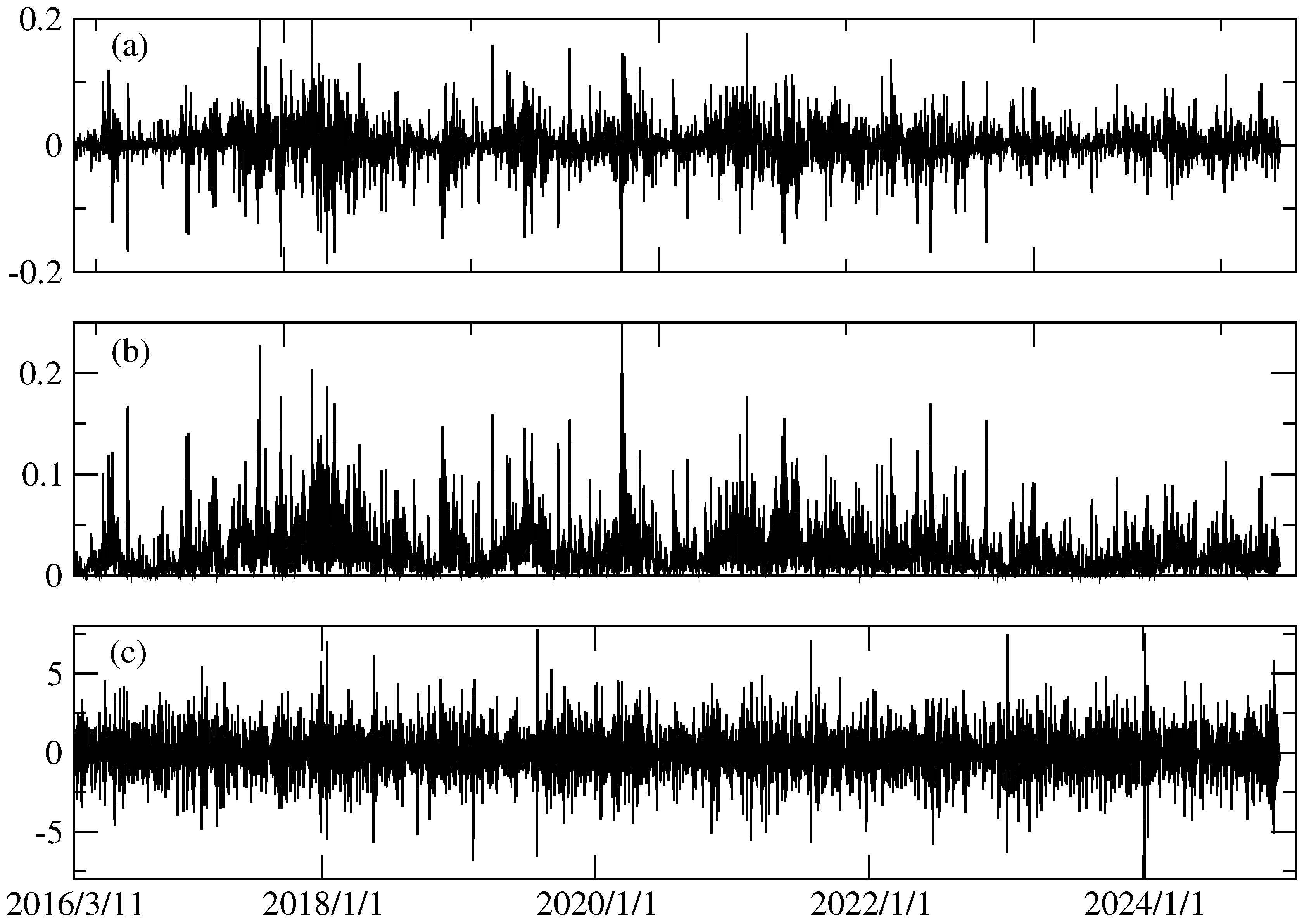
Figure 1. Time series of (a) returns, (b) absolute returns, and (c) volatility increment.
Jrfm 18 00237 g001
Figure 2. Time evolution of h ( 2 ) for Bitcoin returns, computed using window sizes of 1.5, 2, 3, 4, and 5 years.
Jrfm 18 00237 g002
Figure 3. Time evolution of h ( 2 ) for return, absolute return, and volatility increment time series in the stock market. (a) DAX, (b) Nikkei 225, (c) SSE, (d) VIX. The three lines in the plots indicate the financial and pandemic-related dates as follows. (black) The bankruptcy of the Lehman Brothers (15 September 2008). (blue) The WHO declared COVID-19 a pandemic (11 March 2020). (magenta) The WHO declared the end of the COVID-19 pandemic (5 May 2023).
Jrfm 18 00237 g003
Figure 4. Time evolution of h ( 2 ) for return, absolute return, and volatility increment time series in the stock market, from 1 July 2019 to 19 January 2024. (a) DAX, (b) Nikkei 225, (c) SSE, (d) VIX. The two dotted lines indicate the pandemic-related dates as follows. (blue) The WHO declared COVID-19 a pandemic (11 March 2020). (magenta) The WHO declared the end of the COVID-19 pandemic (5 May 2023).
Jrfm 18 00237 g004
Figure 5. Time evolution of h ( 2 ) for return, absolute return, and volatility increment time series in the cryptocurrency market. (a) Bitcoin, (b) Ethereum. The two lines indicate the pandemic-related dates as follows. (blue) The WHO declared COVID-19 a pandemic (11 March 2020). (magenta) The WHO declared the end of the COVID-19 pandemic (5 May 2023).
Jrfm 18 00237 g005
Figure 6. The Hurst exponent h ( 2 ) and its values multiplied by four.
Jrfm 18 00237 g006
Figure 7. Time evolution of Δ h ( n ) for Bitcoin returns, computed for n = 1 , 2 , 3 , 4 , and 5.
Jrfm 18 00237 g007
Figure 8. Same as Figure 4 but for time evolution of Δ h ( 5 ) .
Jrfm 18 00237 g008
Figure 9. Same as Figure 5 but for time evolution of Δ h ( 5 ) .
Jrfm 18 00237 g009
Figure 10. Comparison of Δ h ( 5 ) and Δ α ( 5 ) for Bitcoin. (a) Returns, (b) absolute returns, (c) volatility increment.
Jrfm 18 00237 g010
Table 1. Descriptive statistics of (a) returns, (b) absolute returns, and (c) volatility increment. The values in the parentheses are statistical errors estimated using the jackknife method.
MeanVarianceKurtosisSkewness
(a)DAX 2.2 ( 2.1 ) × 10 4 2.2 ( 3 ) × 10 4 8.3(1.6)−0.28(14)
Nikkei 225 0.9 ( 1.8 ) × 10 4 2.2 ( 3 ) × 10 4 8.6(2.3)−0.3(1)
SSE 1.3 ( 2.5 ) × 10 4 2.2 ( 4 ) × 10 4 8.3 ( 9 ) 0.35 ( 21 )
VIX 0.6 ( 2.7 ) × 10 4 4.8 ( 5 ) × 10 3 9(2)0.96(20)
Bitcoin 1.7 ( 1.0 ) × 10 3 1.4 ( 2 ) × 10 3 16(10)−0.80(75)
Ethereum 1.6 ( 1.3 ) × 10 3 2.6 ( 4 ) × 10 3 12.5 ( 5.6 ) 0.57 ( 63 )
(b)DAX 1.03 ( 8 ) × 10 2 1.1 ( 2 ) × 10 4 14(3)2.6(3)
Nikkei 225 1.05 ( 7 ) × 10 2 1.1 ( 2 ) × 10 4 17(6)2.7(7)
SSE 1.02 ( 9 ) × 10 2 1.2 ( 2 ) × 10 4 13(1)2.6(1)
VIX 4.8 ( 2 ) × 10 2 2.2 ( 3 ) × 10 3 20(6)2.8(4)
Bitcoin 2.4 ( 3 ) × 10 2 7.9 ( 1.9 ) × 10 4 33(24)3.4(1.2)
Ethereum 3.4 ( 3 ) × 10 2 1.44 ( 23 ) × 10 4 24(14) 3.1 ( 7 )
(c)DAX 0.05 ( 6.82 ) × 10 4 2.6(1)4.36(18) 2.7 ( 3.2 ) × 10 2
Nikkei 225 6.4 ( 7.2 ) × 10 4 2.70(7)4.6(1) 3.9 ( 4.5 ) × 10 2
SSE 4.5 ( 7.3 ) × 10 4 2.95(11)4.4(3) 0.6 ( 2.6 ) × 10 2
VIX 1.0 ( 2.1 ) × 10 3 2.25 ( 7 ) 3.9(1) 2.6 ( 2.7 ) × 10 2
Bitcoin 0.07 ( 1.86 ) × 10 3 2.86(7)4.2(3) 3.1 ( 4.0 ) × 10 2
Ethereum 0.6 ( 1.7 ) × 10 3 2.6(1)3.58(17) 1.2 ( 5.8 ) × 10 2
Table 2. Hurst exponents of returns for Bitcoin and Ethereum before and during the COVID-19 periods.
PeriodBitcoinEthereum
1 January 2017–31 December 2019
(before COVID-19)
0.5780.605
1 January2020–30 December 2020
(during COVID-19)
0.4930.561
Table 3. The COVID-19 pandemic’s impact on return, absolute return (AR), and volatility increment (VI) time series. The meanings of the symbols are as follows. ◯: impact observed, ×: no impact observed, ∆: impact unclear.
DAXNikkei 225SSEVIXBitcoinEthereum
Returns h ( 2 ) negative×positive××
Returns Δ h ( 5 ) negativepositivenegativenegative
AR h ( 2 ) negativenegativenegativenegative××
AR Δ h ( 5 ) negativepositivenegative
VI h ( 2 ) ××××××
VI Δ h ( 5 ) ××××××
Disclaimer/Publisher’s Note: The statements, opinions and data contained in all publications are solely those of the individual author(s) and contributor(s) and not of MDPI and/or the editor(s). MDPI and/or the editor(s) disclaim responsibility for any injury to people or property resulting from any ideas, methods, instructions or products referred to in the content.