There was an error in the original publication (Leightner, 2024). Reiterative Truncated Projected Least Squares (RTPLS) uses Equation (10) to estimate −α0^, which is then used in Equation (8) to calculate a separate slope estimate for every observation
(dYt/dXt)^ = Yt/Xt − α0^/Xt
(dYt/dXt)^ − Yt/Xt = − α0^/Xt (8) rearranged
My mistake was to calculate the slope estimates as Yt/Xt + α0^/Xt instead of as Yt/Xt − α0^/Xt. Adding, instead of subtracting, would have been correct if the dependent variable when estimating Equation (10) had been Yt/Xt − (dYt/dXt)^. Thus, the mistake was due to confusion about how Equation (8) was rearranged to create Equation (10).
This mistake only affected the empirical estimates. The mistake did not change my major conclusions.
A correction has been made to the Abstract; Section 1, 4th paragraph; Section 2, 3rd sentence of the second paragraph; Section 2, 4th sentence of the last paragraph; Section 3, last paragraph; Section 4, last paragraph; Table 1, Figures 6 and 7; Section 5 and Note 3.
The corrected version of the Abstract appears below:
This paper uses Reiterative Truncated Projected Least Squares to estimate the effects of US monetary and fiscal policy on Australia using quarterly data between 1960 and 2022. When Australia had a fixed exchange rate (1960–1983), US fiscal and US monetary policies were usually positively correlated with Australia’s GDP (except for 1975–1976, and the second quarter of 1981), which fits the predictions of the small-country IS/LM/BP model with relatively immobile capital. When Australia had a flexible exchange rate (1984–2022), US fiscal policy was always positively correlated with Australia’s GDP, but US monetary policy was usually negatively correlated with Australia’s GDP (except for parts of 1984, 1988–1990, 2012–2015, and 2017), which fits the predictions of the large-country IS/LM/BP model.
The corrected version of Section 1, 4th paragraph appears below:
Applying RTPLS to quarterly data for Australia from 1984 to 2022 (when Australia had a flexible exchange rate), produces estimates where increases in US money supply decreased Australia’s GDP (except for parts, or all of 1984, 1988–1990, 2012–2015, and 2017), while increases in US government consumption always increased Australia’s GDP. This result is exactly what the large-country IS/LM/BP model would predict; however, the negative effect of an increase in US money supply noticeably declined over time. Likewise, when Australia had a fixed exchange rate (from 1960 to 1983), the effect of an increase in the US money supply was positive (except for parts, or all of, 1975–1976) as predicted by the large-country IS/LM/BP model (although, again, the size of this effect diminished over time). Contrary to the large-country IS/LM/BP predictions, US fiscal policy also had a positive effect on Australia’s GDP when Australia had a fixed exchange rate between 1960 and 1983; a result that fits the predictions of the small-country IS/LM/BP model where Australia had relatively immobile capital.
The corrected version of Section 2, 3rd sentence of the second paragraph appears below:
BP shifts to the right because a lower exchange rate is consistent with a lower level of imports, which is consistent with an increase in GDP.
The corrected version of Section 2, 4th sentence of the last paragraph appears below:
Australia’s BP line shifts horizontally to the left because a higher exchange rate is consistent with more imports, which is consistent with a lower GDP (Y).
The corrected version of Section 3, last paragraph appears below:
In Equation (11), ‘s’ is the standard deviation, ‘n’ is the number of observations, and tn−1,α/2 is taken off the standard t table for the desired level of confidence. In this paper, I used an RTPLS estimate along with the two RTPLS estimates that preceded it, the two RTPLS estimates that followed it, and a 95% confidence level to create a moving confidence interval (much like a moving average) for any given set of RTPLS estimates. This 95% confidence interval can be interpreted as meaning there is only a 5% chance that the true value lies outside of this range, given how much omitted variables have varied, both immediately before and immediately after this estimate.
The corrected version of Section 4, last paragraph appears below:
The RTPLS process was applied four times, once for each of Equations (12)–(15) using the data that corresponded to each individual equation. The RTPLS estimates that were produced are plotted over time in Figures 6 and 7. Table 1 gives the 95% confidence intervals for the RTPLS estimates as calculated by Equation (11).

Table 1.
95% Confidence intervals for the change in Australia’s GDP (Y) due to US fiscal (USG) and monetary (USM1) policies.
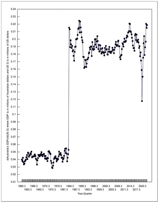
Figure 6.
Change in Australia’s GDP due to a change in US Government consumption.
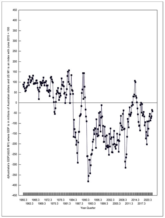
Figure 7.
Change in Australia’s GDP due to a change in US money supply.
The corrected version of Section 5 appears below:
The first numbers given in Table 1 can be interpreted as follows. We can be 95% sure that a one-million-dollar increase (decrease) in US government consumption in the first quarter of 1961 was correlated with an increase (decrease) in Australia’s GDP of between 0.034 and 0.042 million Australian dollars (AUD 34,000 to 42,000), holding constant Australia’s own fiscal and monetary policies, and holding constant US monetary policy. Likewise, we can be 95% sure that a one-unit increase (decrease) in the US money supply index in the first quarter of 1961 was correlated with an increase (decrease) in Australia’s GDP of between 60.2 to 96.6 million Australian dollars, holding constant Australia’s own fiscal and monetary policies, and holding constant US government consumption. The US money supply index in the first quarter of 1961 was 4.6842; a one unit increase in that number would be equal to a 21.35 percent increase in the US money supply.
The variations in the RTPLS estimates shown in Table 1 and Figures 6 and 7 are due to omitted variables. These omitted variables might include changes in the monetary policy targets (inflation, nominal income, and unemployment), as explained by Berger and Wagner (2006). These omitted variables also might include changes in the terms of trade, the degree to which countries are interconnected through international channels, the degree of market power, the relative economic size of countries as discussed by Corsetti and Pesenti (2001), and/or changing nominal rigidities interacting with other changing distortions as shown by Obstfeld and Rogoff (2002). These omitted variables might also include changes in the imperfections of capital markets, changes in how expectations are formed, changes in the policy multipliers of different countries, changes in the degree of capital mobility between countries, and/or changes in the interactions of labor unions across international borders as presented by Carlberg (2005).
The confidence intervals shown in Table 1 and the local minimum RTPLS estimates depicted in Figures 6 and 7 strongly correlate with the world’s recessions. Kose et al. (2020) dates four periods of global recession during the time examined in this paper, namely 1975, 1982, 1991, and 2009. To these four periods, I also added 2020 due to the COVID-19 recession (noting, Kose et al. 2020 only examined the data through to 2019). During each of these global recessions, the positive effects on Australia’s GDP of US expansionary fiscal and monetary policy weakened, and the negative effects strengthened. Thus, during global recessions when Australia most needs stronger positive spillover effects and weaker negative spillover effects from US expansionary economic policy, Australia gets the opposite of what the country needs.
Specifically in the first quarter of 1974, d(Australia’s GDP)/d(US G) hit a local maximum of 0.0511, which fell to 0.0287 in the fourth quarter of 1975. Meanwhile, d(Australia’s GDP)/d(US M1) fell from +126.1 to −53.29. In the first quarter of 1982, d(Australia’s GDP)/d(US G) was 0.0542, which fell to 0.0376 in the first quarter of 1983. Meanwhile, d(Australia’s GDP)/d(US M1) fell from +151.5 to −1.423. In the fourth quarter of 1989, d(Australia’s GDP)/d(US G) was 0.216, but it fell to 0.163 in the fourth quarter of 1991. Meanwhile, the negative effects of expansionary US monetary policy strengthened, going from d(Australia’s GDP)/d(US M1) = +143.7 (confidence interval of 15.2 to 150) to −381.1. In the fourth quarter of 2008, d(Australia’s GDP)/d(US G) was 0.190, which fell to 0.178 in the fourth quarter of 2009. Meanwhile, d(Australia’s GDP)/d(US M1) fell from −36.83 to −314.9. Finally, in the third quarter of 2018, d(Australia’s GDP)/d(US G) was 0.196, which fell to 0.150 by the third quarter of 2020. Meanwhile, d(Australia’s GDP)/d(US M1) went from −44.38 to −159.6.
As predicted by the large-country IS/LM/BP model, d(Australia’s GDP)/d(US M1) was significantly greater than zero when Australia had a fixed exchange rate, except for the first quarter of 1975 to the third quarter of 1976, and the second quarter of 1981, both of which occurred during world recessions. Also, as predicted by the large-country IS/LM/BP model, d(Australia’s GDP)/d(US M1) was significantly less than zero when Australia had a flexible exchange rate, except for 1984, the second quarter of 1988 to the fourth quarter of 1990, the fourth quarter of 2012 to the third quarter of 2015, and the first to the third quarter of 2017. When under a flexible exchange rate, d(Australia’s GDP)/d(US M1) was significantly less than zero (at a 95% confidence level) 81.6 percent of the time. The exceptions to the large-country IS/LM/BP predictions for d(Australia’s GDP)/d(US M1) are probably due to the influence of omitted variables that are not considered in the normal large-country IS/LM/BP model.
As Table 1 shows, all of the d(Australia’s GDP)/d(US G) estimates were significantly greater than zero using a 95% confidence interval (the minimum value for these intervals always exceeded zero). In contrast, the large-country IS/LM/BP model would predict a negative value for d(Australia’s GDP)/d(US G) when Australia had a fixed exchange rate, and a positive value under a flexible exchange rate. Thus, the positive value for d(Australia’s GDP)/d(US G) when Australia had a fixed exchange rate, does not fit the large-country IS/LM/BP predictions. However, it does fit the small-country IS/LM/BP predictions for a country with relatively immobile capital. When a country (the US) increases its government spending (G), two domestic results happen that can affect the international market: (1) the resulting increase in US GDP should increase US imports, and (2) the resulting increase in US interest rates should cause an increased inflow of foreign capital, and a decreased outflow of US capital; this should put upward pressure on the value of the US dollar. In the large-country IS/LM/BP model, the interest rate effect dominates (overwhelms) the increased imports effect. However, in the small-country IS/LM/BP model with relatively immobile capital, the increased imports effect dominates (overwhelms) the interest rate effect. Thus the small-country IS/LM/BP model, with relatively immobile capital for Australia, is consistent with the US increasing government spending causing an increase in US GDP, which causes an increase in US imports, which causes an increase in Australia’s exports, which leads to Australia’s GDP rising producing a positive relationship between US government spending and Australia’s GDP.
Most importantly, this explanation for the positive relation between US government spending and Australia’s GDP, when Australia had a fixed exchange rate, is consistent with historical facts. As the Bank for International Settlements (n.d.) explains, Australia has struggled with controlling capital flows into Australia under a fixed exchange rate. To limit capital inflows, Australia has used different types of capital controls, shifted to what the Australian dollar was pegged, and revalued the Australian dollar several times. These types of policies should make capital less mobile into Australia. The Bank for International Settlements (n.d., p. 3) states, ‘During 1976, controls on capital flows were eased as capital flows failed to match large current account deficit, despite a sizeable positive interest rate differential’. This statement implies that in 1976, the US increase in imports (increasing Australian exports) dominated over the interest rate effect, contrary to the large-country IS/LM/BP model, but consistent with the small-country IS/LM/BP model for a country with relatively immobile capital.
The Bank for International Settlements (n.d., p. 10) description of capital flows, when Australia had a flexible exchange rate, is consistent with the large-country IS/LM/BP model: ‘Capital flows freely to and from Australia and both inflows and outflows have been large, reflecting Australia’s close integration into the world economy.’ Thus, the small-country IS/LM/BP model with relatively immobile capital, fits Australia when Australia had a fixed exchange rate and strong capital controls (1960–1983), and the large-country IS/LM/BP model fits Australia when Australia had a flexible exchange rate and no capital controls (1984–2022).
The average values for d(Australia’s GDP)/d(US G) when Australia had a fixed exchange rate and flexible exchange rate were 0.0433 and 0.191 respectively, representing a 4.4 fold increase.
The corrected version of Note 3 appears below:
Most simulations testing RTPLS tested situations where the true slope was always either positive or negative. Leightner (2015) ran a few simulations that showed that RTPLS could handle situations where omitted variables sometimes make the true slope positive and, at other times, negative. However, even in those cases (where the true slope is sometimes positive and sometimes negative), a researcher must decide which slope sign dominates. The researcher must then use the dominant slope direction when peeling the data.
The author states that the scientific conclusions are unaffected. This correction was approved by the Academic Editor. The original publication has also been updated.
Reference
- Leightner, J. (2024). How Australia has been affected by US monetary and fiscal policies: 1960 to 2022. Journal of Risk and Financial Management, 17(3), 96. [Google Scholar] [CrossRef]
Disclaimer/Publisher’s Note: The statements, opinions and data contained in all publications are solely those of the individual author(s) and contributor(s) and not of MDPI and/or the editor(s). MDPI and/or the editor(s) disclaim responsibility for any injury to people or property resulting from any ideas, methods, instructions or products referred to in the content. |
© 2025 by the author. Licensee MDPI, Basel, Switzerland. This article is an open access article distributed under the terms and conditions of the Creative Commons Attribution (CC BY) license (https://creativecommons.org/licenses/by/4.0/).