Abstract
This paper uses Reiterative Truncated Projected Least Squares to estimate the effects of US monetary and fiscal policy on Australia using quarterly data between 1960 and 2022. When Australia had a fixed exchange rate (1960–1983), US fiscal and US monetary policies were usually positively correlated with Australia’s GDP (except for 1975–1976, and the second quarter of 1981), which fits the predictions of the small-country IS/LM/BP model with relatively immobile capital. When Australia had a flexible exchange rate (1984–2022), US fiscal policy was always positively correlated with Australia’s GDP, but US monetary policy was usually negatively correlated with Australia’s GDP (except for parts of 1984, 1988–1990, 2012–2015, and 2017), which fits the predictions of the large-country IS/LM/BP model.
1. Introduction
A simple large-country IS/LM/BP model (Mundell–Fleming Model) assumes perfect capital mobility—thus, a decrease in country 1’s interest rate will cause capital to flow from country 1 into country 2, putting upward pressure on country 2’s exchange rate and downward pressure on country 1’s exchange rate (Daniels and VanHoose 2004). This model would predict an increase in country 1’s money supply (where country 1 has a flexible exchange rate) will lead to a decrease in GDP for countries with flexible exchange rates and increases in GDP for countries with fixed exchange rates. The opposite effects are predicted if country 1 increases government spending—the GDP of countries with fixed exchange rates will fall, and the GDP of countries with flexible exchange rates will rise. Leightner (forthcoming) tested these predictions using data from the Republic of Korea (South Korea) from 1962 to 1997 when Korea had a fixed exchange rate and from 1998 to 2022 when Korea had a flexible exchange rate. Leightner’s (forthcoming) empirical estimates for Korea fit the four predictions of the large-country IS/LM/BP model. This paper replicates Leightner’s (forthcoming) analysis using Australian data, confirming his flexible exchange rate results but finding important differences between when Korea and Australia had fixed exchange rates.
Since the year 2000, the theoretical literature on international financial connections and possible policy coordination between countries has become much more complex than the simple large-country IS/LM/BP model in Daniels and VanHoose (2004). Corsetti and Pesenti (2001) present a model with monopolistic production specific to one country, countries of different sizes, adjusting terms of trade, and inflation shocks. Obstfeld and Rogoff (2002) show that nominal rigidities that interact with other distortions (like imperfect capital markets and monopolies) make the international coordination theory ambiguous. Carlberg (2005) investigates (1) the effects of ‘going cold turkey’ or taking a gradualist approach to international cooperation, (2) the effects of imperfect capital markets, (3) two, three, or more world regions, (4) adaptive or rational expectations, (5) different countries having different policy multipliers, (6) different degrees of capital mobility between countries, (7) different sizes of countries, (8) labor unions that cooperate or compete across international borders, and (9) inflation. Berger and Wagner (2006) develop a two-country model with vertical trade, sticky prices, and different monetary targeting goals (money supply, nominal income, consumer price index, producer price index). Sugandi (2020) explains a dynamic stochastic general equilibrium model with four economic agents (firms, households, government, and central banks) and two factors of production. He shows that the relative size of the coordinating countries is a dominant variable.
Developing a model that would include all the variables found to be important in the above-cited theoretical literature, collecting the data required by that all-inclusive model, and then estimating that model using traditional statistical techniques would be impossible. Even the first step of that process—accurately modeling everything that can affect exchange rates, GDP, and interest rates and can account for any possible market distortion and heterogeneous countries—is impossible. Cogan et al. (2010) show that how models are constructed can dramatically affect the empirical estimates produced. Using the same data, Cogan et al. (2010) found very different government spending multipliers when a Taylor Keynesian model versus a Romer–Bernstein Keynesian model is used. Fortunately, Leightner et al. (2021) and Leightner (2015) explain Reiterative Truncated Projected Least Squares (RTPLS)—a solution to the omitted variables problem of regression analysis that makes estimations possible without having to develop and justify complete macroeconomic models.
Applying RTPLS to quarterly data for Australia from 1984 to 2022 (when Australia had a flexible exchange rate), produces estimates where increases in US money supply decreased Australia’s GDP (except for parts, or all of 1984, 1988–1990, 2012–2015, and 2017), while increases in US government consumption always increased Australia’s GDP. This result is exactly what the large-country IS/LM/BP model would predict; however, the negative effect of an increase in US money supply noticeably declined over time. Likewise, when Australia had a fixed exchange rate (from 1960 to 1983), the effect of an increase in the US money supply was positive (except for parts, or all of, 1975–1976) as predicted by the large-country IS/LM/BP model (although, again, the size of this effect diminished over time). Contrary to the large-country IS/LM/BP predictions, US fiscal policy also had a positive effect on Australia’s GDP when Australia had a fixed exchange rate between 1960 and 1983; a result that fits the predictions of the small-country IS/LM/BP model where Australia had relatively immobile capital.
This paper not only adds to the literature on how the USA’s fiscal and monetary policies affect other countries, it also adds to the literature on Australia’s exchange rate, which includes the following: Chowdhury (2012) studies how Australia’s real exchange rate is affected by Australia’s terms of trade, government expenditures, net foreign liabilities, interest rate differential, openness to trade, and labor productivity. Atif et al. (2012) include many of the same variables but also find that political events and external shocks affect Australia’s exchange rate. Manalo et al. (2015) find that a ten percent appreciation of Australia’s real exchange rate that is unrelated to interest rate differentials or the terms of trade lowers real GDP by 0.3 percent over a one-to-two-year period.
The remainder of this paper is organized as follows: Section 2 presents a simplified explanation of the IS/LM/BP predictions (simplified means feedback effects from Australia to the US, which normally are in a large-country IS/LM/BP model, are not explained). Section 3 explains the statistical technique used in this paper. Section 4 explains the data and how RTPLS will be specifically applied to those data. Section 5 presents and discusses the empirical results. Section 6 concludes.
2. The Large-Country IS/LM/BP Predictions
In the simplest large-country IS/LM/BP model, capital is assumed to be perfectly mobile for both countries, which gives both countries the same horizontal BP line fixed at the world’s interest rate. In Figure 1, the US’s IS curve is shifted right by an increase in government spending (G). The resulting increase in US interest rates causes capital to move from Australia into the US, which puts upward pressure on the US exchange rate and downward pressure on Australia’s exchange rate. When Australia had a fixed exchange rate (1960–1983), the Australian government used its foreign reserves to purchase the resulting surplus of Australian dollars on the international market. The purchased Australian dollars were pulled out of circulation, reducing Australia’s money supply. A reduction in Australia’s money supply shifted Australia’s LM curve to the left, causing a fall in Australia’s GDP (Y). In Figure 1, the LM curve would shift to the left until a new three-way equilibrium is found.1 Thus, the US increasing government spending causes a reduction in the GDP of countries with fixed exchange rates.
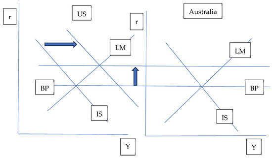
Figure 1.
Large-country IS/LM/BP with the US increasing government spending.
When Australia had a flexible exchange rate (1984–2022), the story was the same as given above, up to what happens to Australia’s exchange rate. Under a flexible exchange rate, Australia’s exchange rate (US $/Australian $) falls, causing BP to shift horizontally to the right, which pulls IS with it to the right. BP shifts to the right because a lower exchange rate is consistent with a lower level of imports, which is consistent with an increase in GDP. However, in the perfect capital mobility case, the horizontal BP shifts horizontally along itself, making the shift invisible. However, the fall in the exchange rate causes exports to increase and imports to decrease, causing aggregate demand and IS to shift to the right. Thus, in Figure 1, the international adjustment for Australia under a flexible exchange rate would appear as the IS curve shifting to the right to create a new three-way equilibrium, which would increase Australia’s GDP (Y). Therefore, the US increasing government spending causes reductions in the GDPs of countries with fixed exchange rates and increases in the GDPs of countries with flexible exchange rates.
Figure 2 shows that the US increasing its money supply reduces the GDPs of countries with flexible exchange rates and increases the GDPs of countries with fixed exchange rates—the opposite of what Figure 1 showed. The US increasing its money supply shifts the US LM curve to the right, decreasing US interest rates. Capital moves from countries with lower interest rates (now the US) into countries with relatively higher interest rates (Australia), putting downward pressure on the US exchange rate and upward pressure on Australia’s exchange rate. When Australia had a fixed exchange rate (1960–1983), a shortage of Australian dollars in the international money market emerged. To maintain its fixed exchange rate, Australia eliminated this shortage by printing more Australian dollars and exchanging them for US dollars (or some other major foreign currency). This process increased Australia’s money supply, shifting Australia’s LM curve to the right in Figure 2 (until there is a new three-way equilibrium), resulting in an increase in Australia’s GDP (Y). Thus, when Australia had a fixed exchange rate, the US increasing its money supply caused an increase in Australia’s GDP, but the US increasing government spending caused a reduction in Australia’s GDP.
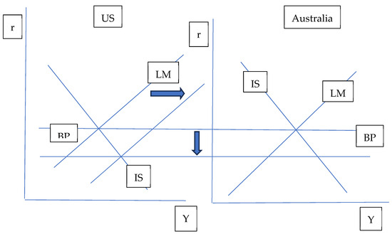
Figure 2.
Large-country IS/LM/BP with the US increasing its money supply.
The opposite of the above result happened when Australia had a flexible exchange rate (1984–2022) and the US increased its money supply. The beginning of the story for the flexible exchange rate is the same as the beginning of the story for the fixed exchange rate up to what happens to Australia’s exchange rate. Under a flexible exchange rate, the US dollar per Australian dollar rises, shifting Australia’s BP horizontally to the left, which pulls Australia’s IS curve to the left also. Australia’s BP line shifts horizontally to the left because a higher exchange rate is consistent with more imports, which is consistent with a lower GDP (Y). However, a horizontal line shifting horizontally along itself is impossible to see. The rise in Australia’s exchange rate reduces Australia’s exports and increases Australia’s imports, causing Australia’s aggregate demand and IS curves to shift left. Australia’s IS curve will shift left until there is a new three-way equilibrium in Figure 2. This leftward shift in Australia’s IS curve decreases Australia’s GDP (Y). Thus, increases in the US money supply caused a reduction in Australia’s GDP when Australia had a flexible exchange rate (1984–2022) but increased Australia’s GDP when Australia had a fixed exchange rate (1960–1983). This paper empirically tests these predictions using the statistical technique explained in Section 3.
3. Methods
In order to estimate the effects on Australia’s GDP of US monetary and fiscal policy when Australia had a fixed exchange rate (1960–1983) and then when Australia had a flexible exchange rate (1984–2022), a researcher would either need to (1) develop, justify, and estimate every equation in an international model that included every force that could affect Australia’s and the US’s GDP, exchange rates, interest rates, etc. or (2) forego the modeling of the thousands of forces needed for option (1) and the gathering of the data for that model and instead use a solution to the omitted variables problem of regression analysis. Reiterative Truncated Projected Least Squares (RTPLS) is a solution to the omitted variables problem. RTPLS produces a separate slope estimate for every observation where differences in these slope estimates are due to omitted variables. By plotting RTPLS estimates over time, a researcher can see how omitted variables have affected the estimated relationship over time, and the researcher does not need to build and justify a model in the process. Thus, RTPLS estimates are not model-dependent. How RTPLS solves the omitted variables problem is explained next.
If a researcher estimates Equation (1) while ignoring Equation (2), the resulting estimate of β1 is a constant when, in truth, β1 varies with qt (via Equation (2). This constitutes an ‘omitted variable’ problem where ‘qt’ represents the combined influence of all omitted variables plus any random variation in β1 itself, Y is the dependent variable, X is the included independent variable, and u is the random error.
Yt = α0 + β1Xt + u
β1 = α1 + α2qt
One convenient way to model the omitted variable problem is to combine Equations (1) and (2) to produce Equation (3).
Yt = α0 + α1Xt + α2 Xt qt + ut.
Equation (7) can be derived from Equation (3) as shown below.
(dYt/dXt)True = α1 + α2qt Derivative of (3)
Yt/Xt = α0/Xt + α1 + α2qt + ut/Xt (3) divided by X
α1 + α2qt = Yt/Xt − α0/Xt − ut/Xt (5) rearranged
(dYt/dXt)True = Yt/Xt − α0/Xt − ut/Xt From (4) and (6)
If an estimate for α0 could be found, then it could be used to calculate a separate slope estimate for each observation using Equation (8). The error due to such a procedure is shown in Equation (9). The ut/Xt term in Equation (9) should be extremely small because random error, ut, is usually tiny relative to the size of Xt, making ut/Xt even smaller (if Xt is greater than one). Thus, the accuracy of calculating a separate slope estimate for each observation using Equation (8) depends primarily upon the accuracy of the α0 estimate.
(dYt/dXt)^ = Yt/Xt − α0^/Xt
(dYt/dXt)True − (dYt/dXt)^ = (α0^ − α0)/Xt − ut/Xt From (7) and (8)
Branson and Lovell (2000) were the first ones to argue that the observations at the top of a scatter plot between a dependent variable (Y) and an independent variable (X) are at the upper frontier of the scatter plot, specifically because variables omitted from the analysis increase Y the most for any given X for those observations. RTPLS projects all observations to the upper frontier, runs a regression through the resulting projected data, and associates the resulting slope estimate with the observations that defined that frontier. The frontier observations are then removed from the data set (but saved in a new data set), and the process is repeated, producing a slope estimate for when omitted variables are at their second most favorable levels. This process is repeated, peeling the data down layer by layer until fewer than ten observations are left. RTPLS then starts over with the entire data set and peels the data up from the bottom, producing another set of layer slopes. Equation (10) is then used with the peeling down and peeling up layer slopes, (dYt/dXt)^, to estimate α0. This α0, along with each Yt and Xt, is plugged into Equation (8) to produce a separate slope estimate for each observation. Leightner (2015) explains the math that underlies RTPLS.
(dYt/dXt)^ − Yt/Xt = − α0^/Xt (8) rearranged
Leightner (2015) and Leightner et al. (2021) report simulation tests that show that when the importance of omitted variables is 100 times as big as the random error, using OLS while ignoring omitted variables produces approximately 35 times the error of RTPLS. When the importance of omitted variables is 10 times as big as random error, then using OLS while ignoring omitted variables produces approximately 3.8 times the error of RTPLS.
Confidence intervals for RTPLS estimates can be calculated using the central limit theorem.
Confidence interval = mean ± (s/√n)tn−1, α/2
In Equation (11), ‘s’ is the standard deviation, ‘n’ is the number of observations, and tn−1,α/2 is taken off the standard t table for the desired level of confidence. In this paper, I used an RTPLS estimate along with the two RTPLS estimates that preceded it, the two RTPLS estimates that followed it, and a 95% confidence level to create a moving confidence interval (much like a moving average) for any given set of RTPLS estimates. This 95% confidence interval can be interpreted as meaning there is only a 5% chance that the true value lies outside of this range, given how much omitted variables have varied, both immediately before and immediately after this estimate.
4. The Data
Monthly data were downloaded from the OECD database on the USA’s and Australia’s money supply (M1) indices, where June 2015 was equal to 100. Quarterly data for M1 were calculated by averaging the three monthly values for each quarter. Quarterly data on Australia’s gross domestic product (GDP) and USA and Australian government consumption (G) also were downloaded from the OECD data website. The GDP and government consumption data were in millions of US dollars for the USA and in millions of Australian dollars for Australia.
Figure 3 depicts the money supply indices for Australia and the USA. Figure 3 shows that from 2007 to 2019, Australia and the USA increased their money supplies at approximately the same rate. However, in response to the coronavirus, the USA increased its money supply much more than Australia did. Figure 4 depicts the ratio of government consumption to GDP for Australia and the USA (which produced a more interesting comparative graph than just plotting government consumption over time). Government consumption as a percent of GDP is on a downward trend for the USA but an upward trend for Australia. In the third quarter of 1960, government consumption as a percent of GDP was 10.77 percent for Australia but 15.08 percent for the USA. However, by the end of 2022, this ratio had changed to 21.04 percent for Australia and 14.15 percent for the USA. Both Australia and the USA increased government spending as a percent of GDP during the onset of the coronavirus.
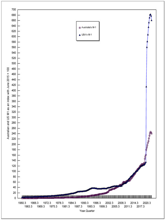
Figure 3.
The money supply (M-1) indices for Australia and the USA.
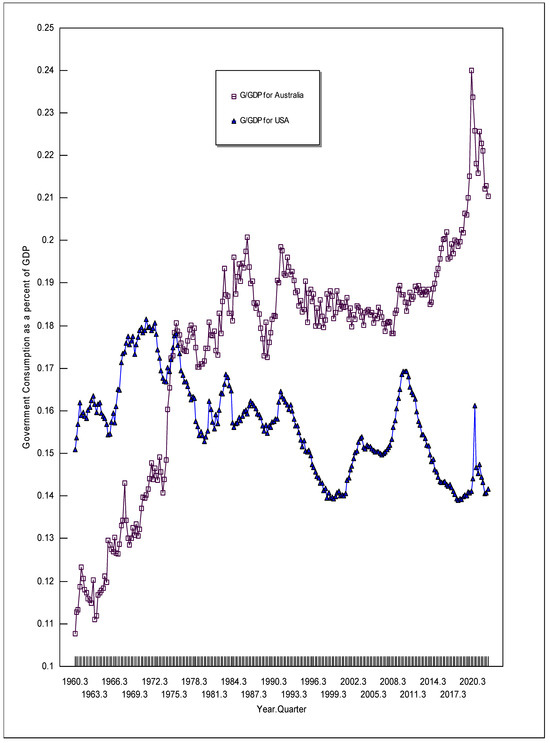
Figure 4.
Government consumption as a percent of GDP for Australia and the USA.
As explained above, the large-country Mundell–Fleming model would predict that USA monetary policy and fiscal policy would have opposite effects on Australian GDP when Australia had a fixed (1960–1983) versus flexible (1984–2022) exchange rate. However, a fixed exchange rate that is adjusted optimal amounts very frequently can act similar to a flexible exchange rate. Figure 5 shows that Australia did not adjust its fixed exchange rate optimal amounts frequently enough to imitate a flexible exchange rate. The earliest exchange rate data that I could find for Australia was from the Reserve Bank of Australia, and it started in July of 1969. Figure 5 shows a clear difference between before and after December 1983. Australia’s exchange rate clearly varied up and down much more after December 1983 than before. After December 1983, Australia’s exchange rate shows no periods of “stair steps” like staying at 1.19 US dollar per Australian dollar for December 1971 to November 1972, or 1.42 US dollar per Australian dollar for February 1973 to August 1973, or 1.49 US dollar per Australian dollar for September 1973 to August 1974. Although the stair-step pattern in Australia’s exchange rate stopped in August 1974, the remainder of Australia’s fixed exchange rate regime followed a downward trend that was not repeated during Australia’s flexible exchange rate regime in terms of the size of the fall or consistency of the fall.2
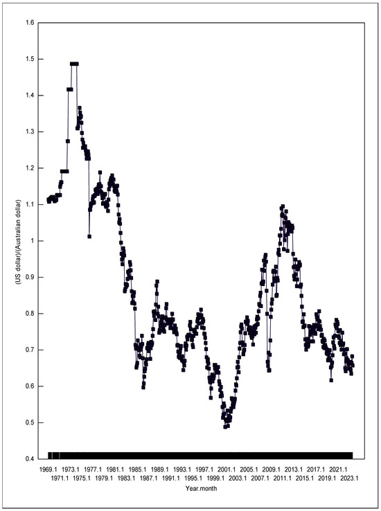
Figure 5.
The US dollar per Australian dollar exchange rate.
Some additional explanation is needed for how RTPLS is applied specifically to the data described immediately above. As explained in Section 2, RTPLS involves peeling the data down layer by layer. The top layer corresponds to when omitted variables are at their most favorable levels (where favorable means increasing the dependent variable the most). The second layer corresponds to when omitted variables are at their second most favorable levels, etc. Before peeling the data, it must be decided whether the layers represent a positive relationship between the dependent variable (Y) and the included independent variable (X) or a negative relationship 3. If the relationship between Y and X is negative, then all values of Y (but not X) should be multiplied by negative one and a constant added to make all of the Y values positive again. This process changes the true negative slope into a positive slope without changing the absolute value of that slope. Once the RTPLS process is completed, the RTPLS estimates will need to be remultiplied by negative one to change them back into negative values. A researcher can either use theory or run a preliminary OLS regression to decide if a positive or negative relationship should be used. In this paper, a preliminary regression was used (but that preliminary regression produced the signs theory would predict in three out of four cases).
The preliminary regression for when Australia had a fixed exchange rate (1960–1983) produced the following results with an R Squared of 0.999 (t statistics are given in parentheses under the estimates: * indicates 95 percent confidence the true coefficient is not zero and ** indicates 99 percent confidence, AG = Australia’s government consumption, AM1 = Australia’s Money Supply, USM1 = US Money Supply, and USG = US government consumption):
Australia’s GDP = −887.77 + 3.1634 AG + 4729.2 AM1 + 62.582 USM1 + 0.046437 USG
(−2.041 *) (20.111 **) (8.439 **) (0.2946) (2.253 *)
(−2.041 *) (20.111 **) (8.439 **) (0.2946) (2.253 *)
The preliminary regression for when Australia had a flexible exchange rate (1984–2022) produced the following results (R Squared of 0.997).
Australia’s GDP = 18,179 + 4.0251AG − 182.58 AM1 − 66.978 USM1 + 0.19435 USG
(−2.104 *) (12.132 **) (−1.247) (−3.909 **) (8.235 **)
(−2.104 *) (12.132 **) (−1.247) (−3.909 **) (8.235 **)
In order to see how omitted variables have affected d(Australia’s GDP)/d(USA’s G) and d(Australia’s GDP)/d(USA’s M1) under Australia’s fixed then flexible exchange rates, the influence of the other included independent variables was purged from the data on Australia’s GDP (the dependent variable, Y) before RTPLS was used (Leightner 2015). Specifically, and based upon the above OLS preliminary regressions, the dependent variable used in the RTPLS process for d(Australia’s GDP)/d(USA’s G) from 1960 through 1983 is given in Equation (12), and for 1984 through 2022 is given in Equation (13). The dependent variable used in the RTPLS process for d(Australia’s GDP)/d(USA’s M1) from 1960 through 1983 is given in Equation (14), and for 1984 through 2022 is given in Equation (15).
Y purged = Australia’s GDP − [3.1634 AG + 4729.2 AM1 + 62.582 USM1]
Y purged = Australia’s GDP − [4.0251AG − 182.58 AM1 − 66.978 USM1]
Y purged = Australia’s GDP − [3.1634 AG + 4729.2 AM1+ 0.046437 USG]
Y purged = Australia’s GDP − [4.0251AG − 182.58 AM1 + 0.19435 USG]
The RTPLS process was applied four times, once for each of Equations (12)–(15) using the data that corresponded to each individual equation. The RTPLS estimates that were produced are plotted over time in Figure 6 and Figure 7. Table 1 gives the 95% confidence intervals for the RTPLS estimates as calculated by Equation (11).
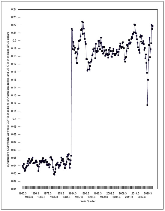
Figure 6.
Change in Australia’s GDP due to a change in US Government consumption.
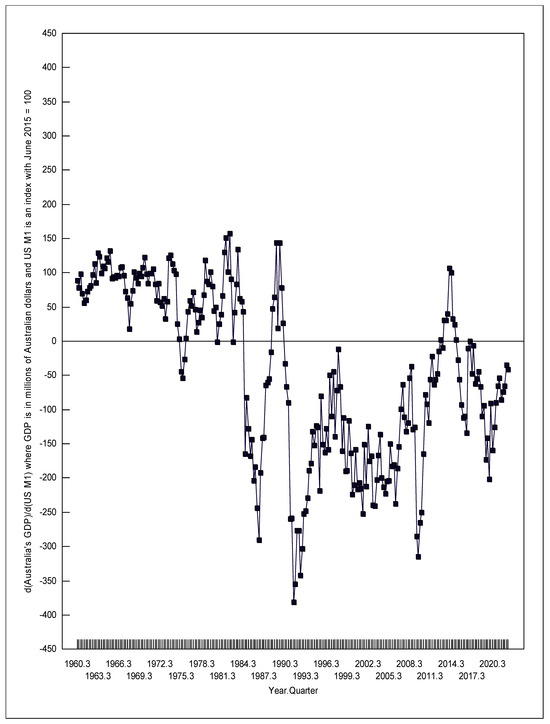
Figure 7.
Change in Australia’s GDP due to a change in US money supply.

Table 1.
95% Confidence intervals for the change in Australia’s GDP (Y) due to US fiscal (USG) and monetary (USM1) policies.
5. Results
The first numbers given in Table 1 can be interpreted as follows. We can be 95% sure that a one-million-dollar increase (decrease) in US government consumption in the first quarter of 1961 was correlated with an increase (decrease) in Australia’s GDP of between 0.034 and 0.042 million Australian dollars (AUD 34,000 to 42,000), holding constant Australia’s own fiscal and monetary policies, and holding constant US monetary policy. Likewise, we can be 95% sure that a one-unit increase (decrease) in the US money supply index in the first quarter of 1961 was correlated with an increase (decrease) in Australia’s GDP of between 60.2 to 96.6 million Australian dollars, holding constant Australia’s own fiscal and monetary policies, and holding constant US government consumption. The US money supply index in the first quarter of 1961 was 4.6842; a one unit increase in that number would be equal to a 21.35 percent increase in the US money supply.
The variations in the RTPLS estimates shown in Table 1 and Figure 6 and Figure 7 are due to omitted variables. These omitted variables might include changes in the monetary policy targets (inflation, nominal income, and unemployment), as explained by Berger and Wagner (2006). These omitted variables also might include changes in the terms of trade, the degree to which countries are interconnected through international channels, the degree of market power, the relative economic size of countries as discussed by Corsetti and Pesenti (2001), and/or changing nominal rigidities interacting with other changing distortions as shown by Obstfeld and Rogoff (2002). These omitted variables might also include changes in the imperfections of capital markets, changes in how expectations are formed, changes in the policy multipliers of different countries, changes in the degree of capital mobility between countries, and/or changes in the interactions of labor unions across international borders as presented by Carlberg (2005).
The confidence intervals shown in Table 1 and the local minimum RTPLS estimates depicted in Figure 6 and Figure 7 strongly correlate with the world’s recessions. Kose et al. (2020) dates four periods of global recession during the time examined in this paper, namely 1975, 1982, 1991, and 2009. To these four periods, I also added 2020 due to the COVID-19 recession (noting, Kose et al. 2020 only examined the data through to 2019). During each of these global recessions, the positive effects on Australia’s GDP of US expansionary fiscal and monetary policy weakened, and the negative effects strengthened. Thus, during global recessions when Australia most needs stronger positive spillover effects and weaker negative spillover effects from US expansionary economic policy, Australia gets the opposite of what the country needs.
Specifically in the first quarter of 1974, d(Australia’s GDP)/d(US G) hit a local maximum of 0.0511, which fell to 0.0287 in the fourth quarter of 1975. Meanwhile, d(Australia’s GDP)/d(US M1) fell from +126.1 to −53.29. In the first quarter of 1982, d(Australia’s GDP)/d(US G) was 0.0542, which fell to 0.0376 in the first quarter of 1983. Meanwhile, d(Australia’s GDP)/d(US M1) fell from +151.5 to −1.423. In the fourth quarter of 1989, d(Australia’s GDP)/d(US G) was 0.216, but it fell to 0.163 in the fourth quarter of 1991. Meanwhile, the negative effects of expansionary US monetary policy strengthened, going from d(Australia’s GDP)/d(US M1) = +143.7 (confidence interval of 15.2 to 150) to −381.1. In the fourth quarter of 2008, d(Australia’s GDP)/d(US G) was 0.190, which fell to 0.178 in the fourth quarter of 2009. Meanwhile, d(Australia’s GDP)/d(US M1) fell from −36.83 to −314.9. Finally, in the third quarter of 2018, d(Australia’s GDP)/d(US G) was 0.196, which fell to 0.150 by the third quarter of 2020. Meanwhile, d(Australia’s GDP)/d(US M1) went from −44.38 to −159.6.
As predicted by the large-country IS/LM/BP model, d(Australia’s GDP)/d(US M1) was significantly greater than zero when Australia had a fixed exchange rate, except for the first quarter of 1975 to the third quarter of 1976, and the second quarter of 1981, both of which occurred during world recessions. Also, as predicted by the large-country IS/LM/BP model, d(Australia’s GDP)/d(US M1) was significantly less than zero when Australia had a flexible exchange rate, except for 1984, the second quarter of 1988 to the fourth quarter of 1990, the fourth quarter of 2012 to the third quarter of 2015, and the first to the third quarter of 2017. When under a flexible exchange rate, d(Australia’s GDP)/d(US M1) was significantly less than zero (at a 95% confidence level) 81.6 percent of the time. The exceptions to the large-country IS/LM/BP predictions for d(Australia’s GDP)/d(US M1) are probably due to the influence of omitted variables that are not considered in the normal large-country IS/LM/BP model.
As Table 1 shows, all of the d(Australia’s GDP)/d(US G) estimates were significantly greater than zero using a 95% confidence interval (the minimum value for these intervals always exceeded zero). In contrast, the large-country IS/LM/BP model would predict a negative value for d(Australia’s GDP)/d(US G) when Australia had a fixed exchange rate, and a positive value under a flexible exchange rate. Thus, the positive value for d(Australia’s GDP)/d(US G) when Australia had a fixed exchange rate, does not fit the large-country IS/LM/BP predictions. However, it does fit the small-country IS/LM/BP predictions for a country with relatively immobile capital. When a country (the US) increases its government spending (G), two domestic results happen that can affect the international market: (1) the resulting increase in US GDP should increase US imports, and (2) the resulting increase in US interest rates should cause an increased inflow of foreign capital, and a decreased outflow of US capital; this should put upward pressure on the value of the US dollar. In the large-country IS/LM/BP model, the interest rate effect dominates (overwhelms) the increased imports effect. However, in the small-country IS/LM/BP model with relatively immobile capital, the increased imports effect dominates (overwhelms) the interest rate effect. Thus the small-country IS/LM/BP model, with relatively immobile capital for Australia, is consistent with the US increasing government spending causing an increase in US GDP, which causes an increase in US imports, which causes an increase in Australia’s exports, which leads to Australia’s GDP rising producing a positive relationship between US government spending and Australia’s GDP.
Most importantly, this explanation for the positive relation between US government spending and Australia’s GDP, when Australia had a fixed exchange rate, is consistent with historical facts. As the Bank for International Settlements (n.d.) explains, Australia has struggled with controlling capital flows into Australia under a fixed exchange rate. To limit capital inflows, Australia has used different types of capital controls, shifted to what the Australian dollar was pegged, and revalued the Australian dollar several times. These types of policies should make capital less mobile into Australia. The Bank for International Settlements (n.d., p. 3) states, ‘During 1976, controls on capital flows were eased as capital flows failed to match large current account deficit, despite a sizeable positive interest rate differential’. This statement implies that in 1976, the US increase in imports (increasing Australian exports) dominated over the interest rate effect, contrary to the large-country IS/LM/BP model, but consistent with the small-country IS/LM/BP model for a country with relatively immobile capital.
The Bank for International Settlements (n.d., p. 10) description of capital flows, when Australia had a flexible exchange rate, is consistent with the large-country IS/LM/BP model: ‘Capital flows freely to and from Australia and both inflows and outflows have been large, reflecting Australia’s close integration into the world economy.’ Thus, the small-country IS/LM/BP model with relatively immobile capital, fits Australia when Australia had a fixed exchange rate and strong capital controls (1960–1983), and the large-country IS/LM/BP model fits Australia when Australia had a flexible exchange rate and no capital controls (1984–2022).
The average values for d(Australia’s GDP)/d(US G) when Australia had a fixed exchange rate and flexible exchange rate were 0.0433 and 0.191 respectively, representing a 4.4 fold increase.
6. Conclusions
This paper added to the literature in several ways. It is only the second paper to empirically test the large-country IS/LM/BP (Mundell–Fleming) predictions for a country that switched from a fixed to a flexible exchange rate. The first empirical test of this model (Leightner forthcoming) used data from Korea and found that all four IS/LM/BP predictions fit the data—(1, 2) expansionary US monetary policy increased Korea’s GDP when Korea had a fixed exchange rate but decreased Korea’s GDP when Korea had a flexible exchange rate, and (3, 4) increases in US fiscal policy reduced Korea’s GDP when Korea had a fixed exchange rate and increased Korea’s GDP when Korea had a flexible exchange rate. This paper confirmed these results for when Australia had a flexible exchange rate but found that both expansionary US fiscal and monetary policy increased Australia’s GDP when Australia had a fixed exchange rate. Although inconsistent with a ‘large’-country IS/LM/BP model, the Australia-under-a-fixed-exchange-rate results are consistent with a ‘small’-country IS/LM/BP model where capital is relatively immobile. Furthermore, an assumption of relatively immobile capital fits the historical record for Australia when it had a fixed exchange rate. Therefore, this paper adds to the literature by being the first paper to produce evidence that the large-country IS/LM/BP model predictions do not fit every country that has a fixed exchange rate.
Leightner (forthcoming) and this paper are also the first two papers to hold some independent variables constant when using Reiterative Truncated Projected Least Squares (RTPLS). Most importantly, this paper found that during world recessions, the positive effects of expansionary US fiscal and monetary policies on Australia’s GDP diminish while the negative effects of expansionary US fiscal and monetary policies increase. Thus, just when Australia most needs positive spillover effects from expansionary US economic policies, these effects decline. The empirical estimates provided in this paper should help Australian authorities manage Australia’s economy in such a way that accounts for the effects of US policies on Australia’s GDP.
Funding
This research received no external funding.
Data Availability Statement
The data are freely available through the OECD data webpage.
Acknowledgments
I appreciate Eric Jenkins downloading and organizing these data for me. I especially appreciate him finding a way to change data that are presented as text into numerical format.
Conflicts of Interest
The author declares no conflicts of interest.
Notes
| 1 | The large-country IS/LM/BP model is more complex than presented here in that what happens in Australia would have feedback effects on the US. In a more complex IS/LM/BP model, the world interest rate would end up somewhere between the initial and final interest rates shown in Figure 1, and the shifts would be more complex than what is presented here. However, the model as presented here explains the major reasons for the IS/LM/BP predictions, which is what is needed for this paper. |
| 2 | According to the Bank for International Settlements (n.d.), the Australian dollar was fixed to the British pound from 1931 to 1971, the US dollar from 1971 to 1974, and a basket of trade-related currencies from 1974 to 1976. The reason Figure 5 does not show a “stair step” pattern for the US$/(Australian dollar) after August 1974 is because Australia was no longer pegging just to the US dollar. In November 1976, Australia devalued its dollar by 17.5 percent relative to its basket of currencies. From 1976 to 1983, Australia used a crawling peg. However, Figure 5 clearly shows that even when Australia was using a crawling peg, it was not changing its exchange rate optimal amounts frequently enough to imitate a flexible exchange rate. |
| 3 | Most simulations testing RTPLS tested situations where the true slope was always either positive or negative. Leightner (2015) ran a few simulations that showed that RTPLS could handle situations where omitted variables sometimes make the true slope positive and, at other times, negative. However, even in those cases (where the true slope is sometimes positive and sometimes negative), a researcher must decide which slope sign dominates. The researcher must then use the dominant slope direction when peeling the data. |
References
- Atif, Syed Muhammad, Moldir Sauytekova, and James Macdonald. 2012. The Determinants of Australian Exchange Rate: A Time Series Analysis. MPRA Paper No. 12309. Available online: https://mpra.ub.uni-muenchen.de/42309/ (accessed on 5 July 2023).
- Bank for International Settlements. n.d. Australia’s Experience with Capital Flows under Different Exchange Rate Regimes: Note for the CGFS Working Group on Capital Flows to Emerging Market Economies. Available online: https://www.bis.org/publ/cgfs33rba.pdf (accessed on 5 July 2023).
- Berger, Wolfram, and Helmut Wagner. 2006. International Policy Coordination and Simple Monetary Policy Rules. IMF Working Paper WP/06/164. Washington, DC: International Monetary Fund. [Google Scholar]
- Branson, Johannah, and C. A. Knox Lovell. 2000. Taxation and Economic Growth in New Zealand. In Taxation and the Limits of Government. Edited by Gerald W. Scully and Patrick J. Caragata. Boston: Kluwer Academic, pp. 37–88. [Google Scholar]
- Carlberg, Michael. 2005. International Economic Policy Coordination. Berlin and Heidelberg: Springer. [Google Scholar]
- Chowdhury, Khorshed. 2012. Modelling the dynamics, structural breaks and the determinants of the real exchange rate of Australia. Journal of International Financial Markets, Institutions and Money 22: 343–58. [Google Scholar] [CrossRef]
- Cogan, John F., Tobias Cwik, John B. Taylor, and Volker Wieland. 2010. New Keynesian versus Old Keynesian Government Spending Multipliers. Journal of Economic Dynamics and Control 34: 281–95. [Google Scholar] [CrossRef]
- Corsetti, Giancarlo, and Paolo Pesenti. 2001. Welfare and Macroeconomic Interdependence. Quarterly Journal of Economics 116: 421–45. [Google Scholar] [CrossRef]
- Daniels, Joseph P., and David D. VanHoose. 2004. International Monetary and Financial Economics, 3rd ed. Nashville: South-Western College Press. [Google Scholar]
- Kose, M. Ayban, Naotaka Sugawara, and Marco E. Terrones. 2020. Global Recessions. Policy Research Working Paper 9172, World Bank. Available online: https://documents1.worldbank.org/curated/en/185391583249079464/pdf/Global-Recessions.pdf (accessed on 5 July 2023).
- Leightner, Jonathan E. 2015. The Limits of Fiscal, Monetary, and Trade Policies: International Comparisons and Solutions. Singapore: World Scientific. [Google Scholar]
- Leightner, Jonathan E. Forthcoming. How US Fiscal and Monetary Policy affect the GDP of Countries with Fixed and Flexible Exchange Rate Regimes: Estimates using Korean Data from 1963 to 2022. Journal of Economic Integration.
- Leightner, Jonathan E., Tomoo Inoue, and Pierre Lafaye de Micheaux. 2021. Variable Slope Forecasting Methods and COVID-19 Risk. Journal of Risk and Financial Management 14: 467. [Google Scholar] [CrossRef]
- Manalo, Josef, Dilhan Perera, and Daniel Rees. 2015. Exchange Rate Movements and the Australian Economy. Economic Modelling 47: 53–62. [Google Scholar] [CrossRef]
- Obstfeld, Maurice, and Kenneth Rogoff. 2002. Global Implications of Self-Oriented National Monetary Rules. Quarterly Journal of Economics 117: 503–36. [Google Scholar] [CrossRef]
- Sugandi, E. 2020. Is International Monetary Policy Coordination Feasible for the ASEAN-5+ 3 Countries? Working Paper No. 1135, Asian Development Bank Institute. Available online: https://www.adb.org/sites/default/files/publication/606521/abdi-wp1135.pdf (accessed on 5 July 2023).
Disclaimer/Publisher’s Note: The statements, opinions and data contained in all publications are solely those of the individual author(s) and contributor(s) and not of MDPI and/or the editor(s). MDPI and/or the editor(s) disclaim responsibility for any injury to people or property resulting from any ideas, methods, instructions or products referred to in the content. |
© 2024 by the author. Licensee MDPI, Basel, Switzerland. This article is an open access article distributed under the terms and conditions of the Creative Commons Attribution (CC BY) license (https://creativecommons.org/licenses/by/4.0/).