The t-Distribution in Financial Mathematics and Multivariate Testing Contexts

Abstract

The Student’s t-distribution provides a thematic connection between the historical and technical elements of this paper. The historical section offers a brief account of the early contributions of Chris Heyde and his collaborations with Madan and Seneta in the development of financial mathematics. The technical section focuses on hypothesis testing, motivated by the observation that, in a setting with pairwise exchangeable dependence for test statistics, the cutoff methods proposed by Sarkar and colleagues in 2016 can be viewed as a first iteration of the classical approach developed by Holm in 1979. These methods had already been refined earlier by Seneta and Chen in their work from 1997 and 2005, which laid the foundation for further improvements. Building on this, a new iteration of the Seneta-Chen method is presented, offering enhancements over the Sarkar approach. Numerical and graphical comparisons are provided, focusing on equal tails testing within the multivariate t-distribution framework. While the tabulated results clearly show improvements with the new procedure, the simulated family-wise error rates across varying correlations reveal only minor practical differences between the iterative methods. This suggests that, under suitable conditions, a single iteration suffices in practice. The paper concludes with personal reflections from the first author, sharing memories of Joe Gani and Chris Heyde, in keeping with the commemorative nature of this issue.

1. Dedication

In Memory of Joe Gani and Chris Heyde.

2. Introduction

The t-distribution in its univariate and multivariate forms provides a thematic link to the historical and technical parts of this paper.

Most of the historical material is in Section 2.2, which is a brief account of the confluence and aftermath of the early work of Chris Heyde focused on the univariate t-distribution, and that of Dilip Madan and ES (the first author) focused on its dual, the Variance-Gamma (VG) distribution, both in the setting of financial mathematics.

Most of the technical part is in Section 3 and Section 4. The general context is the step-down procedure of multivariate hypothesis testing when using equicorrelated pairwise dependent test statistics. In Fung and Seneta (2023), the cutoffs of Sarkar et al. (2016) were seen to be a first iteration improvement of Holm’s classical cutoffs (Holm, 1979), under a convexity condition on the copula. The Sarkar et al. (2016) cutoffs (motivated by Seneta and Chen (2005)) improved on those of Seneta and Chen (1997)1  which already improved on those of Holm (1979) by using pairwise dependence.

Section 3 summarizes this general theory, and notes that under the convexity condition on the copula, a first-iteration improvement of the cutoffs of Seneta and Chen (1997) improves those of Sarkar et al. (2016).

The first purpose of our technical part is to express the copula for a two-equal-tails testing procedure in a calculable form, and the familywise error rate (FWER) into a form calculable from repeated simulation of the sample values. The second purpose is to study numerically the degree of improvement of the improved cutoffs, and to compare the relative effectiveness of the two sets of cutoffs using the FWER, in the specific hypothesis testing setting of two equal-tail tests for multivariate equicorrelated t-distribution. This extends the small initial numerical study in Seneta and Chen (2005) and relates in structure to the examples in Sarkar et al. (2016).

2.1. The Multivariate t-Distribution

The multivariate skew equicorrelated t-distribution is a case of the multivariate skew Generalized Hyperbolic distribution, $GH(0,{\mathbf{R}}_{\mathbf{n}},\theta ,p,a,b)$ described by the mean-variance mixing expression

$$\mathbf{X}=\mathit{\mu }+\mathit{\theta }W+W^{{\displaystyle \frac{1}{2}}}\mathbf{Z}$$

(1)

where $\mathit{\mu }={({\mu }_1,{\mu }_2,\dots ,{\mu }_n)}^{\top },\mathit{\theta }={({\theta }_1,{\theta }_2,\dots ,{\theta }_n)}^{\top }$, where $\mathbf{Z}\sim {\mathbb{N}}_{\mathbf{n}}(\mathbf{0},{\mathbf{R}}_{\mathbf{n}})$ is multivariate normal, with

$${\mathbf{R}}_{\mathbf{n}}={\mathbf{I}}_{\mathbf{n}}(1-\rho )+\rho {\mathbf{11}}^{\top },-1/(n-1)<\rho <1,$$

(2)

where $\mathbf{Z}$ and W are independently distributed. The random variable W has a (univariate) Generalized Inverse Gaussian (GIG) distribution, denoted by $GIG(p,a,b)$, that is, it has density

$$\begin{array}{ccc}\hfill f_{GIG}\left(w\right)& =& {\displaystyle \frac{1}{2{\overline{K}}_p(a,b)}}{w}^{p-1}exp(-{\displaystyle \frac{1}{2}}(a^2{w}^{-1}+b^{2}w)),w>0;\hfill \\ & =& 0,\mathrm{otherwise};\hfill \end{array}$$

where

$${\overline{K}}_p(a,b)=\left\{\begin{array}{cc}{\left({\displaystyle \frac{a}{b}}\right)}^p{K}_p\left(ab\right),\hfill & p\in \mathbb{R},\mathrm{if}a,b>0;\hfill \\ b^{-2p}\Gamma \left(p\right)2^{p-1},\hfill & p,b>0,\mathrm{if}a=0;\hfill \\ a^{2p}\Gamma (-p)2^{-p-1},\hfill & a>0\mathrm{and}p<0,\mathrm{if}b=0.\hfill \end{array}\right.$$

(3)

Here, $K_p\left(\omega \right),\omega >0,$ is the modified Bessel function of the second kind (Erdélyi et al., 1954) with index $p\in \mathbb{R}$.

The case $a=0$ encompasses the multivariate skew Variance-Gamma (VG) distribution.

The case $b=0,p=-\nu /2,a=\sqrt{\nu }$, where $\nu$ is a positive integer, corresponds to the multivariate (n-variate) skewed equicorrelated t-distribution for $\mathbf{X}$ in (1) under (2). ($\nu$ is the “number of degrees of freedom” of the marginal t-distribution).

This multivariate distribution is the central hypothesis testing example in Seneta and Chen (2005) and Sarkar et al. (2016) for testing with two tails under the null hypotheses $H_i:{\mu }_i=\theta =0,i=1,\dots n$, and comparing the relative efficacy of the existing and new cutoffs numerically.

2.2. Historical Prelude

This paper as a whole is, however, part of a tribute issue to my (ES) friends Joe Gani and Chris Heyde, so it is necessary to first explain its descent from the setting of financial mathematics, and in particular the impetus and direction to that field of the work of Chris Heyde.

In mid-1979, I had moved to the University of Sydney from the teaching Department of Statistics at the Australian National University, Canberra, where my interest in financial mathematics developed through collaboration with Dilip Madan. Joe Gani asked me to co-edit a Festrschrift volume of papers in honor of Chris Heyde. The following is an extract from my own contribution, (Seneta, 2004), to that volume.

My own interest up to the appearance of Madan and Seneta (1990) had been in the symmetric VG model. Dilip Madan had moved to the University of Maryland at College Park from the University of Sydney, and I was visiting the University of Virginia when we put the last touches to that paper in 1989. After some years of my own inactivity in this area, I became aware of Chris Heyde’s penetration of yet another probabilistic field, that of financial modelling, and asked him to speak at the University of Sydney on 26 March 1999, on what was soon to be published as Heyde (1999). His opinion of the symmetric VG model was that, although it was heavier tailed than the normal, the tails were not heavy enough to account for what were occasionally relatively extreme values of $X_t$; and of course the increments in the VG model had been assumed independent. Although the underlying stochastic process $log(P_t/P_0),t\ge 0,$ was closed under convolution and analytically convenient, a treatment such as he proposed could effectively reconstruct the $\left\{T_t\right\}$ process numerically from data. My occasional visits to Canberra allowed me to learn more about the FATGBM ideology, and to obtain advice from Chris on the statistical fitting of the symmetric VG model. The VG model had continued to be of interest. I had had several inquiries as to how to fit it to real data, and I needed to supervise the fourth-year Honours project2 of Annelies Tjetjep in 2002. My focus was Dilip Madan’s post-1990 successful extension and application of the VG models (see items in the references co-authored by Madan, especially Madan et al. (1998)), where fitting from data as well as modelling are integral issues. Madan et al. (1998), in the guise of its Research Report predecessor, was already described in a monograph (Epps, 2000). Dilip Madan, Wake Epps, and Eckhard Platen very kindly supplied me with current materials and information, as of course did Chris Heyde. The next section considers the procedure and effect of fitting the (general) VG by allowing for dependence of increments while retaining their stationarity. We do not address specifically the issue of adequacy of tail structure of the VG distribution. Important new work by Heyde and Kou (2004) suggests, in any case, that the heavy-tail (power-law) structure is not easily distinguishable in practice from the exponential-tail structure.

It is appropriate to note on this occasion that the papers authored by Hurst, Platen, and Rachev cited were written in Chris Heyde’s Stochastic Analysis Group at the Australian National University, and are closely related to some of his own work, to which we now come.

To explain, let $P_t$ be the price of a risky asset at some time $t\ge 0,$ and assume that $P_t$ follows subordinated geometric Brownian motion. Specifically, we have

$$P_t=P_0{e}^{\mu t+\theta T_t+\sigma B\left(T_t\right)}$$

(4)

where $\mu ,\theta$ and $\sigma >0,$ are constants, and $\left\{B\right(t\left)\right\}$ is standard Brownian motion independent of $\left\{T_t\right\}$, which is a positive, nondecreasing random process with stationary, but not necessarily independent, increments and $T_0=0.$ Denote the identically distributed increments over unit time by ${\tau }_t=T_t-T_{t-1}$; these form a discrete-time stationary process. The corresponding log increments of $P_t$, which can be interpreted as continuously compounded returns, are given by

$$X_t=log{P}_t-log{P}_{t-1}=\mu +\theta {\tau }_t+\sigma (B\left(T_t\right)-B\left(T_{t-1}\right))$$

(5)

Without loss of generality, take $E\left({\tau }_t\right)=1,$ since any scaling can be absorbed into $\theta$ and $\sigma$ as required (assuming that $E\left({\tau }_t\right)<\infty$).

When t is a positive integer, as is appropriate when sampling at equally spaced points of time, the joint probability structure of the $X_t$ is the same as for the model

$$X_t=\mu +\theta {\tau }_t+\sigma {\tau }_t^{{\displaystyle \frac{1}{2}}}{W}_t,t=1,2,\dots ,$$

(6)

where the $W_t,t=1,2,\dots ,$ are NID(0, 1) random variables, independent also of the process $\left\{{\tau }_t\right\}$, $t=1,2,\dots$

The paradigm model for asset price movements, geometric Brownian motion, takes $\theta =0,{\tau }_t=t$ in the above. The model is relatively simple, giving log returns as independent and identically distributed normal random variables. It has a number of shortcomings in the light of typical asset price data, which display the following characteristics as listed in Finlay and Seneta (2006) (see, for example, Heyde and Liu (2001) and the references therein): (i) a leptokurtic distribution (kurtosis greater than three)—higher peaks above the mean, and thicker tails, than a normal distribution; (ii) a heteroscedastic time series (time-dependent variance), unlike the geometric Brownian motion model; (iii) a long-range dependence structure in squared returns, violating the independence assumption; (iv) occasionally skewed distributions as opposed to the symmetry of a normal distribution; (v) little or no autocorrelation present in returns, at least past one or two lags. To deal with some of these issues, Heyde (1999) introduced a subordinator model (a model which gives asset prices as geometric Brownian motion driven by some nondecreasing stochastic ‘activity time’ or ‘market time’ process) based on fractal activity time: the fractal activity time geometric Brownian motion (FATGBM) model.

Heyde and Leonenko (2005)3 expanded on this model to allow for t-distributed asset price increments, which incorporate self-similarity (a scaling property) and long-range dependence (LRD).

On the basis of preprints and reprints of this and related work, in Section 6, entitled ’Student’ processes, of Seneta (2004), it was noted that the distribution of $X_t$ in (6) when $\mu =0=\theta$, and the distribution of ${\tau }_t=T_t-T_{t-1}$ which is the reciprocal (inverse) gamma, is Praetz’s-t distribution.

A multivariate version ${\mathbf{X}}_{\mathbf{t}}$ of (5) is

$${\mathbf{X}}_{\mathbf{t}}=\mu +{\tau }_t\theta +\mathbf{W}\left({\tau }_t{\mathbf{R}}_{\mathbf{n}}\right)$$

(7)

where $\mathbf{W}$ is the multivariate correlated Brownian motion (Wiener process) evaluated at positive integer time points $t,$ univariate ${\tau }_t$ has an inverse gamma distribution, and ${\mathbf{R}}_{\mathbf{n}}={\mathbf{I}}_{\mathbf{n}}(1-\rho )+\rho {\mathbf{11}}^{\top },-1/(n-1)<\rho <1.$ The distribution of ${\mathbf{X}}_{\mathbf{t}}$ is then a skewed equicorrelated multivariate t which at a given time point can be written as (1). All marginal distributions are the same as expressed in (5).

In conclusion to this historical account, after Seneta (2004), univariate theory was developed in a series of papers with Richard Finlay, the first of which was Finlay and Seneta (2006), and the multivariate theory, especially bivariate, with Thomas Fung, one of the first of which was Fung and Seneta (2011).

It is the skewed multivariate t-distribution with which we are concerned in the sequel, although in a context different from the preceding, namely multiple hypothesis testing. However, this different context and the multivariate financial mathematics context have in common the central role played by the Student’s t-copula (see our Section 3.1).

3. Multivariate Hypothesis Testing Context

3.1. The Step-Down Procedure

We consider the multiple test problem when there are n hypotheses $H_1,H_2,\dots ,H_n$, and corresponding p-values $R_1,R_2,\dots R_n,$ assuming the test statistics $Y_1,Y_2,\dots ,Y_n$ are from a continuous distribution. Suppose that in such a multiple test procedure, the property

$$Pr(H_s,s\in I_m,\mathrm{are}\mathrm{accepted}|H_s,s\in I_m\mathrm{are}\mathrm{true})\ge 1-\alpha$$

(8)

holds for a prespecified size of test $\alpha$ (familywise error: FWE) for every $I_m$, where $I_m$ is any non-null subset of $\{1,2,\dots ,n\}$, for every $m=1,2,\dots ,n.$ Then, the FWE is said to be strongly controlled.

Let $R_{\left(1\right)},R_{\left(2\right)},\dots ,R_{\left(n\right)}$ be the ordered p-values, and $\Delta \left(i\right),1\le i\le n$ be a strictly increasing sequence of constants, with $0<\Delta \left(i\right)<1,$ for each $i.$ A step-down procedure begins by testing if $R_{\left(1\right)}<\Delta \left(1\right).$ If so, reject $H_{\left(1\right)}$ and go on to test if $R_{\left(2\right)}<\Delta \left(2\right).$ If not, accept all hypotheses. In general, if $R_{\left(i\right)}<\Delta \left(i\right),1\le i\le j-1$, then at step j, the remaining hypotheses are $H_{\left(j\right)},H_{(j+1)},\dots ,H_{\left(n\right)},$ and the inequality next to be checked is $R_{\left(j\right)}<\Delta \left(j\right)$. If it holds, reject $H_{\left(j\right)}$ and continue. Otherwise, accept $H_{\left(j\right)},H_{(j+1)},\dots ,H_{\left(n\right)}.$ The process may continue until a decision is made on the basis of whether $R_{\left(n\right)}<\Delta \left(n\right).$ The step-down procedure of Holm (1979) uses the set of constants

$$\overline{\Delta }\left(i\right)={\displaystyle \frac{\alpha }{n-i+1}},1\le i\le n,$$

(9)

and Holm proved that with these constants, the FWE is strongly controlled.

In the sequel, we shall have that $(Y_i,Y_j),i\ne j,i,j\in I_m$ are exchangeable (so that $(R_i,R_j)$ are also) when $I_m,m\ge 2$ is the index set of assumed true hypotheses, and that their joint bivariate distribution is the same for each such $I_m.$ The marginal distribution of each $R_i,i\in I_m,m\ge 1$ is $U(0,1).$ We shall need the notation

$$H\left(u\right)=Pr(R_1\le u,R_2\le u),u\in (0,1),$$

(10)

Under the above exchangeability setting, Seneta and Chen (1997), in their Sections 5 and 6, showed that then the critical cutoff constants

$$\tilde{\Delta }\left(i\right)={\displaystyle \frac{\alpha +(n_0-1)H\left(\frac{\alpha }{n_0}\right)}{n_0}},$$

(11)

are monotonic increasing with i (that is, decreasing with increasing $n_0$), and the step-down procedure based on them strongly controls the FWE. Moreover, the step-down procedure with these constants provides tighter control on the FWE than Holm’s since

$$\tilde{\Delta }\left(i\right)>\overline{\Delta }\left(i\right)={\displaystyle \frac{\alpha }{n_0}},1\le i\le n-1,\tilde{\Delta }\left(n\right)=\overline{\Delta }\left(n\right)=\alpha .$$

Note that $H\left(u\right),0<u<1,$ is a cdf. It also serves as the copula $C(u_1,u_2)=Pr(R_1\le u_1,R_2\le u_2),0<u_1,u_2<1,$ of the bivariate joint distribution of the exchangeable pair $(X_1,X_2)$, evaluated along the diagonal $u_1=u_2=u.$ In one such application of the Student’s t-copula, Sun et al. (2008) utilized a skewed Student’s t-copula-based ARMA-GARCH model to capture tail dependence and asymmetric correlation, particularly relevant for financial markets, where extreme events and non-elliptical distributions are common.

Sarkar et al. (2016), motivated by Seneta and Chen (2005), made a substantial improvement. They showed, under the condition that $H\left(u\right)$ in (10) is convex in $u\in (0,1),$ that the monotonic increasing (with i) cutoffs

$$\widehat{\Delta }\left(i\right)={\displaystyle \frac{{\alpha }^2/n_0}{G_{n_0}(\alpha /n_0)}},$$

(12)

where

$$G_{n_0}\left(u\right)=n_{0}u-(n_0-1)H\left(u\right),0<u<1,$$

(13)

provide tighter control on the FWE than (11) since they show

$$\widehat{\Delta }\left(i\right)>\tilde{\Delta }\left(i\right),1\le i\le n-1,\tilde{\Delta }\left(n\right)=\overline{\Delta }\left(n\right)=\alpha .$$

Write

$$w_2\left(n_0\right)={\displaystyle \frac{\alpha w_1\left(n_0\right)}{G_{n_0}\left(w_1\left(n_0\right)\right)}},$$

(14)

Clearly, $w_2\left(n_0\right)$ is (12) when $w_1\left(n_0\right)$ is (9);

Fung and Seneta (2023) showed, under the same convexity condition on $H\left(u\right)$, that $w_2\left(n_0\right)$ given by (14) when $w_1\left(n_0\right)$ is (11), provides tighter control on the FWE than (12). This is a consequence of their Theorem 1: since

$$w_1^{*}\left(n_0\right)={\displaystyle \frac{\alpha +(n_0-1)H\left(\frac{\alpha }{n_0}\right)}{n_0}}>{\displaystyle \frac{\alpha }{n_0}}=w_1\left(n_0\right)$$

it follows that

$$w_2^{*}\left(n_0\right)>{\displaystyle \frac{{\alpha }^2/n_0}{G_{n_0}(\alpha /n_0)}}=w_2\left(n_0\right)$$

3.2. Two-Tail Tests

Returning to (1) and (2), we take for $i=1,2,\dots ,n$ our ith null hypothesis to be $H_i:{\mu }_i={\theta }_i=0,$ so that when all $H_i$ are true,

$$\mathbf{X}=\sqrt{W}\mathbf{Z},$$

(15)

and similarly for any subset of indices $\{1,2,\dots ,n\}.$

For a two-sided equal-tails testing procedure, we take as our test statistics $Y_i=\left|X_i\right|,i=1,2.\dots ,n$. Their corresponding p-values $(R_i,R_j),i\ne j,i,j\in I_m$ are then also exchangeable, and their joint bivariate distribution is the same for each such $I_m.$

We shall work, for each of two specified values of n for numerical illustration, with three sets of cutoffs: those given by (11) which we call $w_1\left(n_0\right)$;   those given by $\widehat{\Delta }\left(i\right)$ in (12); and those given by (14) which we call $w_2\left(n_0\right)$. This involves the calculation of

$$H\left(u\left(n_0\right)\right)=Pr(R_1\le u\left(n_0\right),R_2\le u\left(n_0\right)),$$

at $u\left(n_0\right)={\displaystyle \frac{\alpha }{n_0}}$ to produce (11) and $\widehat{\Delta }\left(i\right)$ in (12), and $u\left(n_0\right)=w_1\left(n_0\right)$ to produce $w_2\left(n_0\right)$ for each value of $n_0=n-i+1,i=1,2,\dots ,n.$

We have indicated above that $w_1\left(n_0\right)<\widehat{\Delta }\left(i\right)<w_2\left(n_0\right)$. Our intention is to compare numerically the relative efficacy of $\widehat{\Delta }\left(i\right)$ and $w_2\left(n_0\right)$ as improvements on $w_1\left(n_0\right)$. For eventual use in the verification of convexity, and for numerical calculations in terms of test statistics, we first transform to a bivariate setting.

Since

$$Pr(R_1\le u\left(n_0\right),R_2\le u\left(n_0\right))=Pr(Y_1>x,Y_2>x)\mathrm{where}x=F_X^{-1}(1-{\displaystyle \frac{u\left(n_0\right)}{2}}),$$

(16)

we notice that the right-hand side of (16) may be written as

$$\begin{array}{ccc}\hfill Pr(X_1>x,X_2>x)& +& Pr(X_1>x,X_2<-x)\hfill \\ & +& Pr(X_1<-x,X_2<-x)+Pr(X_1<-x,X_2>x)\hfill \end{array}$$

and then as

$$\begin{array}{ccc}\hfill Pr(X_1>x,X_2>x)& +& Pr(X_1>x,-X_2>x)\hfill \\ & +& Pr(-X_1>x,-X_2>x)+Pr(-X_1>x,X_2>x).\hfill \end{array}$$

Putting $V_i=-X_i,i=1,2$, since $(V_1,V_2)$ has the same joint distribution as $(X_1,X_2)$, and since $(X_1,V_2)$ and $(V_1,X_2)$ have the same joint distribution (namely, the joint distribution of $(X_1,X_2)$ but with the sign of the correlation coefficient reversed), (16) is now

$$Pr\left(\right|X_1|>x,|X_2|>x)=2Pr(X_1>x,X_2>x)+2Pr(X_1>x,V_2>x)$$

(17)

Focus on the first summand on the right. Since

$$\begin{array}{cc}\hfill Pr(X_1>x,X_2>x)& =Pr(-X_1<-x,-X_2<x)=Pr(X_1<-x,X_2<-x)\hfill \\ \hfill & =Pr(X_{\left(2\right)}<-x)\hfill \end{array}$$

where $X_{\left(2\right)}=max(X_1,X_2)$, and since $-x=-F_X^{-1}(1-{\displaystyle \frac{u\left(n_0\right)}{2}})=F_X^{-1}\left({\displaystyle \frac{u\left(n_0\right)}{2}}\right)$, it follows from (15) that

$$Pr(X_1>x,X_2>x)=Pr\left(X_{\left(2\right)}\le F_X^{-1}\left(u\right)\right),$$

(18)

for $u={\displaystyle \frac{u\left(n_0\right)}{2}}.$

To evaluate (17), the calculation of (18) needs to be repeated with $\rho$ replaced by $-\rho$ to give $Pr(X_1>x,V_2>x)$.

It is important to note from the right-hand side of (17) that $Pr\left(\right|X_1|>x,|X_2|>x)$ is symmetric about 0 in the value of $\rho$.

For comparisons of the differential effects of various cutoffs, we use the familywise error rate (FWER) as a function of $\rho$ as the means of comparison. This is in general defined as $Pr(\mathrm{Reject}\mathrm{at}\mathrm{least}\mathrm{one}{H}_i,i=1,2,\dots ,n|H_i,i=1,2,\dots ,n\mathrm{are}\mathrm{all}\mathrm{true})$. Thus, for the step-down procedure

$$\begin{array}{ccc}\hfill \mathrm{FWER}& =& Pr(R_{\left(1\right)}<\Delta \left(1\right)|H_i,i=1,2,\dots ,n\mathrm{are}\mathrm{all}\mathrm{true})\hfill \\ & =& Pr(R_{\left(1\right)}<w_j\left(n\right)|H_i,i=1,2,\dots ,n\mathrm{are}\mathrm{all}\mathrm{true})\hfill \\ & =& Pr\left(\underset{i=1,2,\dots ,n}{max}\right|X_i|>F_X^{-1}(1-{\displaystyle \frac{w_j\left(n\right)}{2}})|H_i,i=1,2,\dots ,n\mathrm{are}\mathrm{all}\mathrm{true})\hfill \end{array}$$

(19)

for fixed $j=1,2$, in terms of sample values $X_i$, $i=1,2,\dots ,n$. The expression (19) may be estimated from repeated simulation of the sample $X_i,i=1,2,\dots ,n$, once $F_X^{-1}(1-{\displaystyle \frac{w_j\left(n\right)}{2}})$ is numerically calculated. For our two sets of cutoffs, $u\left(n\right)={\displaystyle \frac{\alpha }{n}}$ and $u\left(n\right)=w_1\left(n\right)={\displaystyle \frac{\alpha +(n-1)H\left(\frac{\alpha }{n}\right)}{n}}$, respectively.

Finally, the earlier numerical investigations of Seneta and Chen (2005), Sarkar et al. (2016), and Fung and Seneta (2023) have all been in the setting of $\rho >0$.

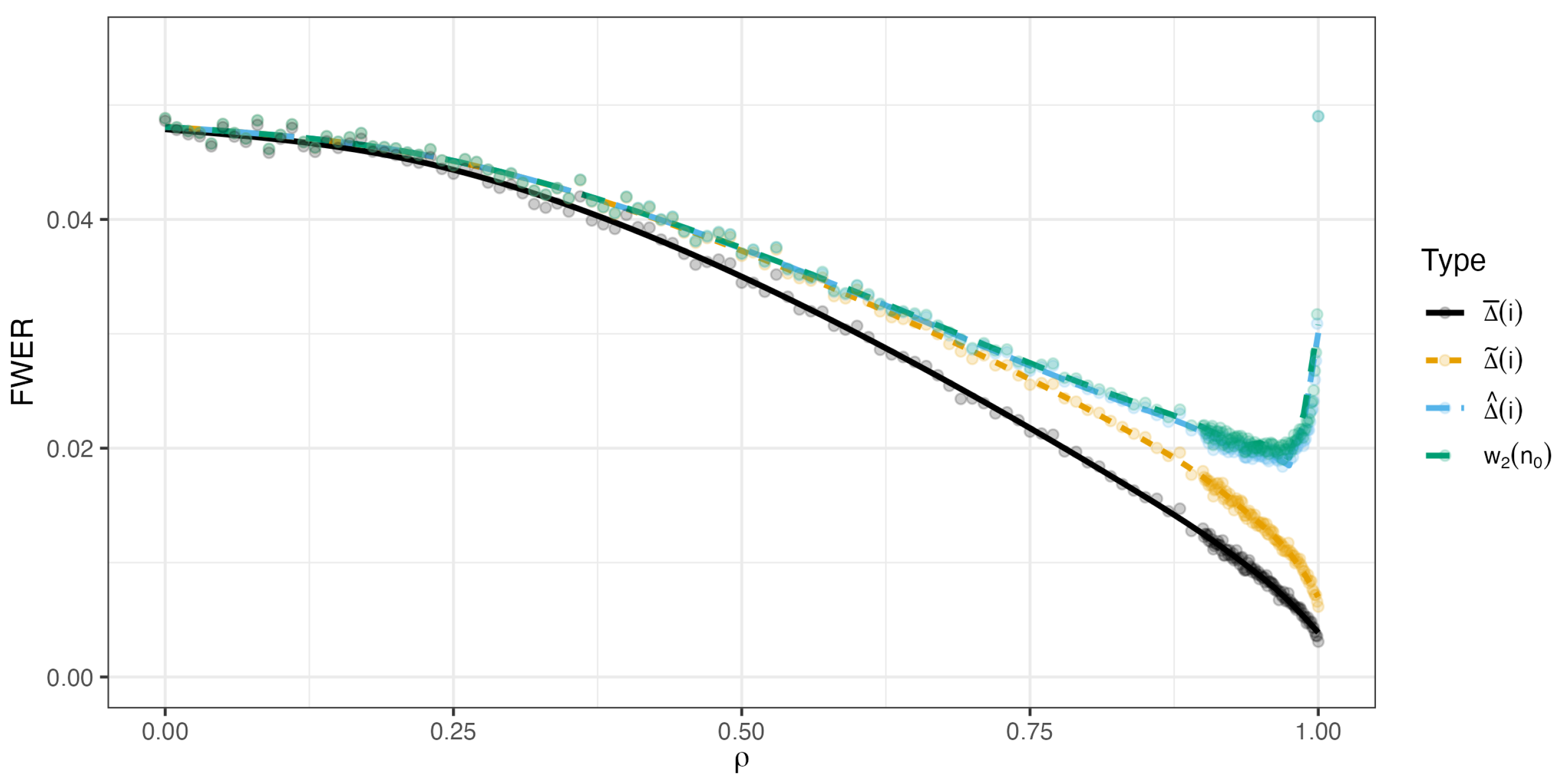
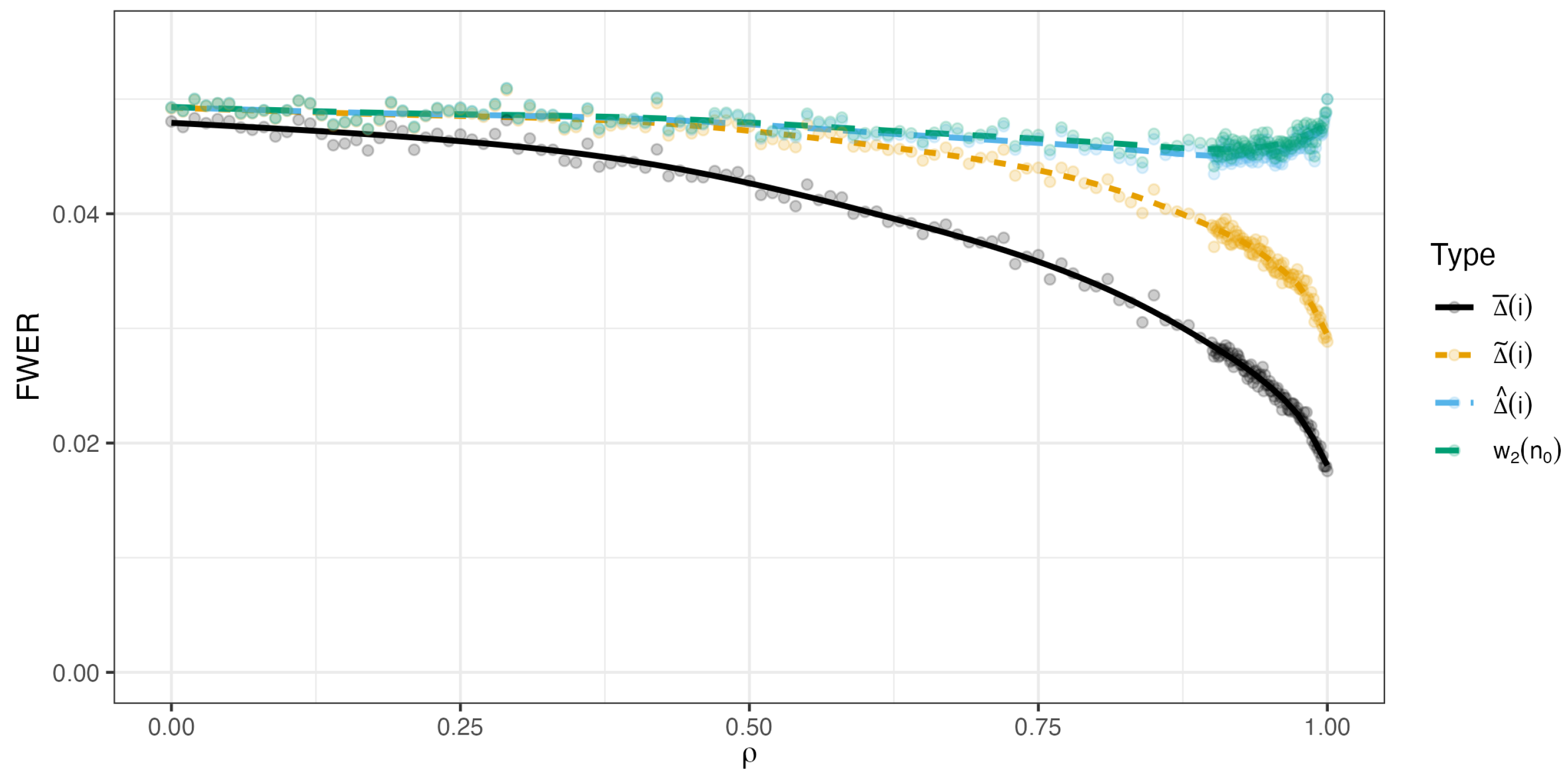
4. Numerical Demonstration. Multivariate t-Distribution

For the specific multivariate t-distribution, Sarkar et al. (2016) proved that on account of the exchangeability, the copula $Pr(F_X\left(X_1\right)\le u,F_X\left(X_2\right))\le u)$ is convex for $u\in (0,1)$, so from (17), $H\left(u\right)$ in (10) is convex as required.

In this section, we present some numerical results to illustrate the theoretical developments discussed earlier.

The work of Seneta and Chen (2005), in its Section 4, provides tabulated results (Table 4), with $\alpha =0.05$ of (11) for $n_0=1,2,\dots ,8$ against $\rho =0.0$, 0.1, …, 0.9, 0.95, 0.99, and 1.00 for test statistic cutoffs from the multivariate normal for a two-tailed test for the zero mean; we extend that analysis. Specifically, we compute (11), (12) and (14) using (11) as $w_1\left(n_0\right)$ under two different multivariate t settings:

• Setting 1: multivariate t with $\nu =64$ and $n=16$.
• Setting 2: multivariate t with $\nu =16$ and $n=3$.

The results are presented in

Table 1. Comparing the cutoffs $\tilde{\Delta }\left(i\right)$ under multivariate t with $n=16$ and $\nu =64$ for various $\rho$.

	$\mathit{\rho }$
${\mathit{n}}_{\mathbf{0}}$	0	0.1	0.2	0.3	0.4	0.5	0.6	0.7	0.8	0.9	0.95	0.99
16	0.00314	0.00315	0.00317	0.00320	0.00326	0.00335	0.00348	0.00369	0.00400	0.00451	0.00493	0.00554
15	0.00335	0.00336	0.00338	0.00342	0.00348	0.00357	0.00372	0.00394	0.00427	0.00481	0.00525	0.00590
14	0.00359	0.00360	0.00362	0.00366	0.00373	0.00383	0.00399	0.00422	0.00458	0.00516	0.00563	0.00631
13	0.00387	0.00388	0.00390	0.00395	0.00402	0.00413	0.00430	0.00456	0.00494	0.00555	0.00605	0.00678
12	0.00419	0.00420	0.00423	0.00428	0.00436	0.00448	0.00467	0.00494	0.00535	0.00601	0.00655	0.00733
11	0.00458	0.00459	0.00462	0.00467	0.00476	0.00490	0.00510	0.00540	0.00584	0.00656	0.00714	0.00797
10	0.00504	0.00505	0.00508	0.00514	0.00524	0.00539	0.00562	0.00595	0.00643	0.00721	0.00783	0.00874
9	0.00560	0.00561	0.00565	0.00572	0.00583	0.00600	0.00625	0.00661	0.00715	0.00800	0.00868	0.00967
8	0.00630	0.00632	0.00636	0.00644	0.00657	0.00677	0.00705	0.00745	0.00804	0.00898	0.00973	0.01081
7	0.00721	0.00723	0.00728	0.00738	0.00752	0.00775	0.00807	0.00852	0.00919	0.01023	0.01107	0.01226
6	0.00842	0.00844	0.00850	0.00862	0.00879	0.00905	0.00942	0.00995	0.01070	0.01188	0.01282	0.01416
5	0.01012	0.01014	0.01022	0.01036	0.01057	0.01088	0.01132	0.01193	0.01280	0.01415	0.01521	0.01673
4	0.01266	0.01270	0.01280	0.01297	0.01324	0.01361	0.01414	0.01486	0.01589	0.01745	0.01868	0.02042
3	0.01691	0.01696	0.01709	0.01731	0.01765	0.01812	0.01876	0.01964	0.02086	0.02268	0.02411	0.02611
2	0.02539	0.02545	0.02562	0.02590	0.02632	0.02688	0.02764	0.02864	0.03001	0.03202	0.03356	0.03571
1	0.05000	0.05000	0.05000	0.05000	0.05000	0.05000	0.05000	0.05000	0.05000	0.05000	0.05000	0.05000

,

Table 2. Comparing the cutoffs $\widehat{\Delta }\left(i\right)$ under multivariate t with $n=16$ and $\nu =64$ for various $\rho$.

	$\mathit{\rho }$
${\mathit{n}}_{\mathbf{0}}$	0	0.1	0.2	0.3	0.4	0.5	0.6	0.7	0.8	0.9	0.95	0.99
16	0.00314	0.00315	0.00317	0.00320	0.00326	0.00336	0.00353	0.00381	0.00434	0.00561	0.00739	0.01373
15	0.00335	0.00336	0.00338	0.00342	0.00348	0.00359	0.00377	0.00407	0.00464	0.00599	0.00787	0.01448
14	0.00359	0.00360	0.00362	0.00366	0.00374	0.00385	0.00405	0.00437	0.00498	0.00642	0.00841	0.01532
13	0.00387	0.00388	0.00390	0.00395	0.00403	0.00416	0.00436	0.00472	0.00537	0.00691	0.00903	0.01625
12	0.00419	0.00420	0.00423	0.00428	0.00437	0.00451	0.00474	0.00512	0.00582	0.00748	0.00974	0.01729
11	0.00458	0.00459	0.00462	0.00467	0.00477	0.00493	0.00518	0.00559	0.00636	0.00815	0.01057	0.01847
10	0.00504	0.00505	0.00508	0.00515	0.00526	0.00543	0.00571	0.00617	0.00701	0.00895	0.01154	0.01982
9	0.00560	0.00561	0.00565	0.00573	0.00585	0.00604	0.00635	0.00686	0.00779	0.00991	0.01270	0.02135
8	0.00630	0.00632	0.00637	0.00645	0.00659	0.00681	0.00716	0.00774	0.00877	0.01110	0.01411	0.02313
7	0.00721	0.00723	0.00728	0.00738	0.00755	0.00780	0.00820	0.00885	0.01001	0.01259	0.01585	0.02521
6	0.00842	0.00844	0.00851	0.00863	0.00882	0.00912	0.00959	0.01033	0.01165	0.01451	0.01804	0.02767
5	0.01012	0.01014	0.01022	0.01037	0.01061	0.01097	0.01152	0.01239	0.01389	0.01709	0.02090	0.03060
4	0.01267	0.01270	0.01280	0.01299	0.01328	0.01372	0.01438	0.01541	0.01715	0.02071	0.02473	0.03414
3	0.01692	0.01696	0.01710	0.01734	0.01771	0.01826	0.01907	0.02028	0.02226	0.02609	0.03010	0.03846
2	0.02540	0.02546	0.02563	0.02593	0.02639	0.02704	0.02795	0.02926	0.03126	0.03475	0.03801	0.04375
1	0.05000	0.05000	0.05000	0.05000	0.05000	0.05000	0.05000	0.05000	0.05000	0.05000	0.05000	0.05000

,

Table 3. Comparing the cutoffs $w_2\left(n_0\right)$ when $w_1\left(n_0\right)$ is (11), under multivariate t with $n=16$ and $\nu =64$ for various $\rho$.

	$\mathit{\rho }$
${\mathit{n}}_{\mathbf{0}}$	0	0.1	0.2	0.3	0.4	0.5	0.6	0.7	0.8	0.9	0.95	0.99
16	0.00314	0.00315	0.00317	0.00320	0.00326	0.00337	0.00354	0.00384	0.00440	0.00575	0.00762	0.01422
15	0.00335	0.00336	0.00338	0.00342	0.00349	0.00360	0.00378	0.00410	0.00470	0.00613	0.00811	0.01499
14	0.00359	0.00360	0.00362	0.00366	0.00374	0.00386	0.00406	0.00440	0.00504	0.00657	0.00867	0.01585
13	0.00387	0.00388	0.00390	0.00395	0.00403	0.00416	0.00438	0.00475	0.00544	0.00708	0.00931	0.01680
12	0.00419	0.00420	0.00423	0.00428	0.00437	0.00452	0.00476	0.00516	0.00590	0.00766	0.01004	0.01787
11	0.00458	0.00459	0.00462	0.00468	0.00478	0.00494	0.00520	0.00564	0.00645	0.00835	0.01089	0.01907
10	0.00504	0.00505	0.00508	0.00515	0.00526	0.00544	0.00573	0.00622	0.00711	0.00917	0.01189	0.02044
9	0.00560	0.00561	0.00565	0.00573	0.00585	0.00606	0.00638	0.00692	0.00790	0.01015	0.01308	0.02200
8	0.00631	0.00632	0.00637	0.00645	0.00660	0.00683	0.00719	0.00780	0.00889	0.01136	0.01452	0.02380
7	0.00721	0.00723	0.00728	0.00739	0.00756	0.00782	0.00824	0.00893	0.01015	0.01288	0.01629	0.02589
6	0.00842	0.00844	0.00851	0.00863	0.00883	0.00915	0.00963	0.01042	0.01181	0.01484	0.01853	0.02834
5	0.01012	0.01015	0.01023	0.01038	0.01062	0.01100	0.01157	0.01250	0.01409	0.01746	0.02141	0.03125
4	0.01267	0.01270	0.01281	0.01300	0.01330	0.01376	0.01446	0.01554	0.01738	0.02111	0.02527	0.03473
3	0.01692	0.01697	0.01711	0.01735	0.01774	0.01831	0.01916	0.02044	0.02252	0.02650	0.03061	0.03893
2	0.02541	0.02546	0.02564	0.02595	0.02642	0.02709	0.02804	0.02941	0.03148	0.03506	0.03835	0.04400
1	0.05000	0.05000	0.05000	0.05000	0.05000	0.05000	0.05000	0.05000	0.05000	0.05000	0.05000	0.05000

,

Table 4. Comparing the cutoffs $\tilde{\Delta }\left(i\right)$ under multivariate t with $n=3$ and $\nu =16$ for various $\rho$.

	$\mathit{\rho }$
${\mathit{n}}_{\mathbf{0}}$	0	0.1	0.2	0.3	0.4	0.5	0.6	0.7	0.8	0.9	0.95	0.99
3	0.01718	0.01723	0.01738	0.01763	0.01800	0.01850	0.01916	0.02004	0.02124	0.02299	0.02434	0.02622
2	0.02572	0.02578	0.02595	0.02626	0.02669	0.02728	0.02805	0.02904	0.03038	0.03231	0.03378	0.03582
1	0.05000	0.05000	0.05000	0.05000	0.05000	0.05000	0.05000	0.05000	0.05000	0.05000	0.05000	0.05000

,

Table 5. Comparing the cutoffs $w_2\left(n_0\right)$ when $w_1\left(n_0\right)$ is (11), under multivariate t with $n=3$ and $\nu =16$ for various $\rho$.

	$\mathit{\rho }$
${\mathit{n}}_{\mathbf{0}}$	0	0.1	0.2	0.3	0.4	0.5	0.6	0.7	0.8	0.9	0.95	0.99
3	0.01720	0.01725	0.01741	0.01769	0.01811	0.01872	0.01960	0.02090	0.02296	0.02686	0.03087	0.03904
2	0.02574	0.02580	0.02599	0.02632	0.02681	0.02751	0.02847	0.02982	0.03185	0.03533	0.03852	0.04406
1	0.05000	0.05000	0.05000	0.05000	0.05000	0.05000	0.05000	0.05000	0.05000	0.05000	0.05000	0.05000

and

Table 6. Comparing the cutoffs $w_2\left(n_0\right)$ when $w_1\left(n_0\right)$ is (11) under multivariate t with $n=3$ and $\nu =16$ for various $\rho$.

	$\mathit{\rho }$
${\mathit{n}}_{\mathbf{0}}$	0	0.1	0.2	0.3	0.4	0.5	0.6	0.7	0.8	0.9	0.95	0.99
3	0.01720	0.01726	0.01742	0.01771	0.01815	0.01878	0.01970	0.02105	0.02320	0.02722	0.03130	0.03943
2	0.02575	0.02581	0.02601	0.02635	0.02686	0.02757	0.02856	0.02997	0.03205	0.03560	0.03881	0.04427
1	0.05000	0.05000	0.05000	0.05000	0.05000	0.05000	0.05000	0.05000	0.05000	0.05000	0.05000	0.05000

. Specifically, we first compute (11), (12), and (14) when $w_1\left(n_0\right)$ is (11).

In Setting 1, $n=16$ is as in Sarkar et al. (2016). To explain the other choices in a model framework, we go to Section 4 of Seneta and Chen (2005) for notation and discussion. Consider l treatments (the first of which is a control), and so l treatment groups, each of size J, and consider testing the simultaneous hypotheses $H_i:{\mu }_i-{\mu }_1=0,i=2,\dots ,l$. Then, $n=l-1$, and for the individual (equicorrelated) test statistics $\nu =lJ-l=l(J-1)$. Then, $l=16,J=5$ implies $\nu =64,n=15;$ while $l=4,J=5$ implies $\nu =16,n=3$. Thus, in Setting 2, the values of $\nu$ and n are precisely as in Section 5 of Seneta and Chen (2005),  allowing some of the numerical results there to be cross-checked as well as for the graphic extension of those results.

Table 1, Table 2, Table 3, Table 4, Table 5 and Table 6 demonstrate that (14) when $w_1\left(n_0\right)$ is (11) provides the tightest control on familywise error (FWE) among the three cutoffs.

Sarkar et al. (2016) presented a graphical comparison of the effect of their cutoff points (12) with those using (11) in the two-tailed setting with $n=16$. Here, we extend this by graphically comparing the FWER resulting from each of four sets of cutoff constants: (9), (11), (12), and (14) when $w_1\left(n_0\right)$ is (11). The comparison is made with respect to error rates with increasing the values of $\rho$ under our two multivariate t settings. The results can be found in Figure 1 and Figure 2. All simulations were performed using the R software package (R Core Team, 2023), with one hundred thousand (100,000) independent replications in each case. The independent multivariate t samples were generated with the mvtnorm package version 1.3-3   of Genz et al. (2021). A generalized additive model (GAM) of Wood (2023) was used to smooth the resulting lines. Figure 1 and Figure 2 parallel Figure 1a of Sarkar et al. (2016).

From these two figures, we observe $\tilde{\Delta }\left(i\right)$, $\widehat{\Delta }\left(i\right)$, and $w_2\left(n0\right)$ all provide significant improvement to the Holm values $\overline{\Delta }\left(i\right)$. There is some evidence from the two figures, for future investigation, that the FWER decreases as n increases, when the rest of the settings remain unchanged. Similarly, as $\rho$ increases, the FWER generally decreases for most methods. However, at very high correlation values (such as $\rho \to 1$), $\widehat{\Delta }\left(i\right)$ and $w_2\left(n_0\right)$ exhibit an upward spike towards $\alpha$. This suggests that when the test statistics are perfectly correlated, only $\widehat{\Delta }\left(i\right)$ and $w_2\left(n_0\right)$ appropriately adjust the FWER by collapsing the results.

However, the improvement in FWER due to $w_2\left(n_0\right)$ when $w_1\left(n_0\right)$ is (11) is so slight so as to be almost indistinguishable from $w_2\left(n_0\right)$ when $w_1\left(n_0\right)$ is (9). This is supported by the fact that even at $\rho =0.99$ and $n_0=16$, $w_2\left(n_0\right)$ provides an approximately 3.5% improvement over $\widehat{\Delta }\left(i\right)$.

In summary, our tabulated results demonstrate that (14), paired with (11) as $w_1\left(n_0\right)$, offers the most effective control of familywise error (FWE), particularly for higher values of $\rho$, under multivariate $\mathit{t}$-distributions. The graphical comparison suggests that a single iterative step from $w_1\left(n_0\right)$ to $w_2\left(n_0\right)$ is enough to stabilize the FWER irrespective of the choice of $w_1\left(n_0\right)$. The extent of improvement from $w_1\left(n_0\right)$ to $w_2\left(n_0\right)$ in the Sarkar et al. (2016) setting is remarkable.

Finally, recall that each of the two iterative steps is justified on account of the convex nature of the Student t-copula, a central result of Sarkar et al. (2016).

5. Some Personal Recollections (ES)

5.1. Joe Gani and Chris Heyde, to September, 1974

My first, indirect, contact with Joe Gani (1924–2016) occurred during my M.Sc. research year, 1964, at the University of Adelaide, when my supervisor John Darroch (1930–2024) made me aware of the work on applied probability centered in P.A.P. (Pat) Moran’s department at the Australian National University (ANU), Canberra, and Joe Gani’s intention there to found the Journal of Applied Probability (JAP) as a focus for publication in that subject area. John’s intention was that our work on quasi-stationarity might eventually be published there as it was (Darroch & Seneta, 1965). In 1965, I began work on my PhD in Statistics enrolled in Moran’s ANU Statistics Department in the Research School of Social Sciences, while working in E.J. (Ted) Hannan’s ANU teaching Department in the School of General Studies (SGS). By then, all the illustrious and to-become-illustrious names associated with Moran’s department had left it, including Joe Gani and Chris Heyde (1939–2008), who had been a PhD student there in 1962–1964. Chris’s nominal supervisor had been J.E. (Jo) Moyal (1910–1998), then Reader in the Department, but Chris worked mainly on his own, following some suggestions made to him by Pat Moran.

Joe Gani and Ted Hannan (1921–1994) had been Moran’s first PhD students at ANU, which had been established in 1946 by Act of Australian Federal Parliament as a centrepiece and focal point for Australian research and PhD training. Joe and Ted’s deep friendship and mutual support, personal and academic continued until Ted’s passing. Chris’s relation with Joe was of a deeply loyal and filial nature.

In September 1964, Chris joined Joe Gani, first in the Department of Statistics at Michigan State University (MSU), East Lansing, where JAP was founded. When Joe Gani left MSU to take up the Chair of Probability and Statistics at the University of Sheffield, UK, at the end of 1965, Chris followed him there as a Lecturer. He was soon promoted to Special Lecturer in charge of the Statistical Laboratory at the University of Manchester in 1967, when the Manchester-Sheffield School of Probability and Statistics was formed.

Chris returned to Australia in September 1968 to take up a Readership in Ted Hannan’s Department of Statistics, from which at the time I was absent on a one year’s Study Leave in the UK. My paper (Seneta, 1968) on the sequence of constants $\left\{c_n\right\}$, (later called the “Seneta constants”) giving convergence in distribution of $\left\{Z_n/c_n\right\}$ to a proper non-degenerate random variable W for the supercritical simple (at the time called the Galton–Watson) branching process, without any further conditions, had appeared in that year and Chris had noticed it. I received a letter in Cambridge from Chris that he had strengthened my result to almost sure convergence by noticing that $\left\{exp\left(-Z_n/c_n\right)\right\}$ was a martingale with (obviously) bounded expectation. He published this in the same journal in 1970, and the result, in its variants and extensions became known as the Seneta–Heyde theorem or norming. Since that time, a principal theme of Chris’s work became the theory and use of martingale methods in situations of statistical dependence.

The dominant theme of Chris’s work prior to his return to Canberra in 1968 was the refinement of classical limit theory for sums of independent random variables, involving large and small deviations, rates of convergence and domains of attraction. His note of 1970 stimulated him to develop a theory for the supercritical process theory analogous to the classical rate of convergence theory. There was a continued focus on inference aspects of branching-type processes, which led to an inclination towards a framework of time-series type results, in which his martingale work was hugely influential. One of his favorite papers was a joint paper with Ted Hannan in this framework.

I had returned to Ted Hannan’s department in the first half of 1969, and from that time our friendship and collaboration began.

At the time of Chris’s return to Canberra in 1968, there was still a strong trend of research at ANU into population genetics, originating from Pat Moran’s book on this topic, which had in fact partly motivated me to come to Canberra from Adelaide. Chris’s interest in population genetics was invigorated by my note (Seneta, 1974), which extended, on its anniversary, Malécot’s Markov chain formulation of the Fisher–Wright model to randomly fluctuating population size. The result uses the martingale convergence theorem, whose nature and use by Chris in his 1970 note had made me aware of its power and breadth of application. There followed a wealth of related and more general studies and papers by Chris, a few being collaborative. My fuller appreciation of Chris’s work on branching processes and population genetics is the paper (Seneta, 2010).

Bienaymé

A second major common interest of mine with Chris was history. This evolved from our contact and collaboration on branching processes, and was initially stimulated by two historical papers published in 1966, one in this area by D. G. Kendall, on Galton and Watson’s study of the criticality theorem for branching processes, the other by H.O. Lancaster on forerunners of the Pearson ${\chi }^2$, which noted that the French statistician, I.J. Bienaymé, in a classic paper of 1853 had made considerable contributions to the theory. Lancaster had been Chris’s M.Sc. supervisor at the University of Sydney (and, as it turned out, was to be my predecessor in the Chair of Mathematical Statistics there, to which I came in 1979). It was in the 1853 paper that Bienaymé had anticipated Chebyshev in the discovery of the inequality which should more appropriately be called the Bienaymé–Chebyshev Inequality.

My interest in whether Bienaymé had made other discoveries was aroused. Through Lancaster’s bibliographic work, a list of Bienaymé’s publications was available. Because of the title of one of Bienaymé’s papers of 1845 on the duration of family names, I requested it on an interlibrary loan, and to my amazement, when it arrived, I found that it contained a completely correct (in contrast to Galton and Watson’s) statement of the criticality theorem. I rushed down the passage from my office to Chris’s to share the news, and we planned the future. The immediate result was the note (Heyde & Seneta, 1972), received February 1972. In time it led to the book, (Heyde & Seneta, 1977). And it became more correct to call the simple branching process the Bienaymé–Galton–Watson process.

5.2. September 1974–1993

From September 1974 to July 1981, Joe was back in Australia as Chief of the CSIRO Division of Mathematics and Statistics. The Division was now based in Canberra and located close to ANU.

Ted Hannan had retired as Professor and Head of the SGS Department in 1970, and C.R. (Chip) Heathcote (1931–2016), who like Chris, had been Reader in the Department, was eventually appointed in his place. Chris who had also applied for the position, joined Joe at the CSIRO in January 1975. Ross Maller (the first PhD student to be enrolled in the SGS Department) was one year into his PhD at the time. Chip asked me to take over as Ross’s supervisor for the remaining two or so years of Ross’s candidature. My area of intersection with Ross’s research was regularly varying functions, but Ross needed little supervision, and our relationship was good.

Chris took over as Acting Chief in 1981 when Joe Gani left the Division, until September 1983 when he was appointed Professor and Chairman of the Department of Statistics at the University of Melbourne. The 45th (100th anniversary) World Statistics Congress (WSC) of the International Statistical Institute took place in 1985 in Amsterdam, at which Chris and I had a happy reunion, although I was billeted at Valkenburg, and he, I think, in Maastricht. In particular I remember us at the van Gogh Museum in Amsterdam, commenting on van Gogh’s Sunflowers, and his depiction of people.

In May 1986, Chris returned to the ANU, and was Professor and Head of the ANU Department of Statistics in the Institute of Advanced Studies from July 1986 to December 1988. Chris and I worked together again on history to motivate and jointly guest-edit for Australia’s Bicentenary the Bicentennial History Issue of the Australian Journal of Statistics (Heyde & Seneta, 1988). That was Special Volume 30B of that year. Volume 30A was a Special Volume of “Papers in honour of J. Gani. C.C. Heyde (Editor)”. to which both Chris and I also contributed.

From 1989 to 1992, Chris was the Foundation Dean of the ANU School of Mathematical Sciences (later the Mathematical Sciences Institute). Since 1993, while continuing at ANU, until his death in 2008, he had also been a Professor in the Department of Statistics at Columbia University, New York. He taught there for their Fall semester each year (September to December) till 2007, and was eventually the Director of that university’s Center for Applied Probability.

5.3. Chris Heyde, 1993–2008

The First World Congress on Branching Processes was held in Varna, Bulgaria, on the Black Sea, in 1993 to celebrate the first 150 years of these processes. Chris presided over the opening session, and I was the first speaker (on history). I attended with Malcolm Quine, who had been my first PhD student. Chris later edited the Proceedings.

In 1995, the Christiaan-Huygens Committee on the History of Statistics of the International Statistical Institute (ISI) was reconstituted with Chris as Chair, and members of the committee became actively involved in what was to become the book Statisticians of the Centuries.

Chris was diagnosed with hairy-cell leukemia in about 1997. In one of his periods of rest during remission, at his and Beth’s old home in Aranda, a Canberra suburb, when I called on him during one of my annual visits from Sydney, he told me about this task. This was the first time that I had learned of the hairy-cell leukemia. Our meeting was outside, on a sunny day. He looked fragile, was somewhat disheveled after rest, and said he did not feel up to the task, on which he had already been engaged for some time. He asked me to share the editorial task with him, and insisted on sharing equally the small initial funding grant from the ISI. And so Centuries came to be. Eventually we were joined by P. Crépel, S.E. Fienberg, and Joe Gani as Associate Editors. When the book was about to appear, he expressed to me great relief at having that millstone round his neck removed. The book appeared in 2001, when the world’s attention was focused on 9/11 in the USA.

Soon after the diagnosis, at the award of a D.Sc. Honoris Causa from his Alma Mater, Sydney University, in 1998, I heard Chris give an inspiring speech to the new graduates, on the rewards of a life in science.

Especially memorable was the occasion of the 52nd WSC, 1999, in Helsinki, Finland, before which we made a side trip to St. Petersburg, Russia. In the company of our wives Beth and Ludmilla, and of our statistical colleagues Neville Weber and Mary Phipps, we enjoyed the warm hospitality of Yuri and Larissa Borovskikh, and experienced an adventure at border crossing out of Russia. On the train from St. Petersburg, before the border with Finland, Russian security decided to search Beth and Chris’s baggage for items being taken out illegally. By the end of their search, they were disappointed that all they had found was a dried banana. Chris and Beth loved to repeat that story in later years.

A highlight of my memories of Chris in Australia was the celebration of his 65th birthday at ANU in 2004. In the speech he made that night following dinner at University House, he expressed gratitude for the extra years had been given him, and his happiness at being able to be present.

He had a special dedication to the Australian statistical tradition and activity. In 2005 the 55th WSC was held in Sydney. Chris was to give an invited lecture on the development of Statistics in our Australian state universities at the meeting He prepared this during one of the periodic flare-ups of his leukemia. As on some such occasions before and after, I was happy to play the role of Chris’s back-up system. Joe Gani’s was to be the opening historical talk, but early in the talk something went wrong. Joe, with obvious relief, discarded his notes and spoke impromptu, something at which he was very good.

Chris Heyde, Contact in Final Years

Chris made several visits from Columbia University, New York, to me at the University of Virginia (UVa.), Mr. Thomas Jefferson’s university, in Charlottesville, where I spent a number of semesters teaching. My first visit to U.Va., with my wife, was 1988–89, for the full academic year. Then, I made fall semester visits within 1999–2001, and finally one in 2005.

In one of his talks at UVa., he described himself as a seeker after truth in the proper way to model random fluctuation of financial returns. That was characteristic of the man.

In late 2005, Leonard Scott my friend and colleague in the Mathematics Department, with experience in financial data and mathematics, organized a farewell conference. The following is from the poster:

The Variance Gamma and Related Financial Models. A conference in honor of Eugene Seneta. University of Virginia, Charlottesville, Virginia. 22–23 October 2005. Speakers: Chris Heyde (Columbia University and ANU). Dilip Madan (University of Maryland), Eugene Seneta (University of Sydney)., +2 . Organizers: Patrick Dennis (U.Va.), Jeff Holt (U.Va.), Leonard Scott (U.Va.).

Chris, Dilip, and I also spoke impromptu at that evening’s departmental dinner and party. The warmth and celebration were a joyful time, which lives in my memory. Among the things that Chris said was that I had successfully resisted a departmental farewell at ANU in 1979, and at Sydney University, but Leonard had, most remarkably, succeeded at UVa.

I had, in return, visited Chris in New York during his period at Columbia University. One Sunday, we walked by the foreshore of the Hudson to Grant’s Tomb, and visited an almost deserted Wall Street, where I bought a wallet from a street vendor, a souvenir which I use to this day. In an email to me dated 20 January 2008, when the prognosis for his illness was already quite negative, Chris wrote the following:

Whatever happens, I certainly feel that I have had a fortunate life. I will be happy to have more, but if not, I have had a good innings and can go in peace.

I last saw him at Canberra Hospital on the Friday before his death, in the company of Beth. They were hopeful, but prepared. His mind was clear, and we all spoke lightly of times together past, present and of possible futures.

Chris died in Canberra Thursday 6 March 2008, from the effects of metastatic melanoma.

Joe was too emotionally fragile to prepare a eulogy, and asked me to do it. He was in the front row of the congregation when I read it at the funeral ceremony on 13 March 2008.

I concluded the tribute with the words of St. Paul, which well describe Chris’s life:

I have fought a good fight, I have finished the race, I have kept the faith.

5.4. ES Contact with Joe Gani

I had had almost no personal contact with Joe before I came to Sydney in mid-1979, and my news of Joe was largely through Ted Hannan and Chris. Prior to Sydney, there was some correspondence by mail relating to publications in his beloved creation, the Journal of Applied Probability (JAP), and then its companion journal Advances in Applied Probability, to be dedicated to longer articles. As the first article in 1969 he had kindly published a review paper originating from work around the creation of the norming constants for the supercritical branching process (Seneta, 1968).

He was a kind, generous, accommodating and efficient editor. At the time, the editorial policy was to use just one referee. I remember one occasion when an author had complained very strongly about a negative referee’s report which indeed was very superficial. Joe then sent the paper to me, for a second opinion. I generally never liked refereeing since I felt that I should actually read a submission carefully, and Joe knew it. But indeed, the paper was a good piece of work. Sometimes people took advantage of the journal’s one-referee policy and Joe’s generosity. Joe could become very angry. One occasion was when a young author plagiarized a paper published earlier by another author in an obscure journal, and it was published in JAP before the plagiarism was discovered.

Concerning another occasion, to set the scene, in a late letter to me dated 16 March 2019, John Darroch (1930–2024) wrote “One of Joe’s highly appreciated initiatives [during Joe’s CSIRO period–ES] was to obtain funding to enable overseas statisticians to visit Australia for weeks or months in order to work jointly with their established research colleagues here in Australia”. There were several Russian mathematical statisticians among such visitors. A problem was that such visitors, although provided with travel and accommodation, were not permitted to take any foreign currency out of the Soviet Union. On one occasion, I heard that Joe, taking pity on the penniless visitor, had given him USD 50 from his own pocket. This visitor had promptly spent all the money to buy himself a tennis racquet. It was one of several visitor occasions, even after the collapse of the Soviet Union in 1991, when Joe was very displeased at the exploitation, in ignorance of civilized norms, of his efforts.

5.4.1. 1983–2016, Varanasi, Mathematical Scientist, Doeblin, ANU

Even though from 1981 to 1994, Joe had been at the University of Kentucky, and the University of California at Santa Barbara, he and I got to know each other better from about this time.

There was to be an International Statistical Conference in India in 1983, and, characteristically, Joe was heavily involved in its organization. But something went wrong at the Indian end, and the locale and Indian organization were, fortunately, able to be moved to Varanasi at Banaras Hindu University, through the generosity and work of the local statisticians, under their Head, whose name I am not now sure of (Professor Singh?). I got one side of my clothes covered in mud from a fall outside the conference venue. Joe came to my rescue with particularly useful suggestions in view of my short supply of replacement trousers.

In the early 1980s, my work on history of probability and statistics in the 19th century had begun to focus strongly on the Russian Empire. I had submitted a long paper on this to Archive for History of Exact Sciences. After revision in response to review by a very eminent referee (van der Waerden), who identified himself, I did not hear for a very long time from the editor. In fact, as I learned later, the paper had been accepted, but an acceptance letter from the (at the time shaky) editorial system never arrived, so I had written to withdraw the paper, and turned to Joe who kindly agreed to publish it without further ado in his very personal creation The Mathematical Scientist. It appeared as Seneta (1984).

That particular issue of Joe’s journal marked a high point in my hobby work on history since it also contained the first of my papers on Lewis Carroll, the author of the Alice books, as probabilist. Later, during his years resettled at ANU, Joe asked me, in line with his social organization activities, to give a seminar on Lewis Carroll there. The audience included a large number of ANU’s mathematicians and mathematical statisticians. It was one of the most successful seminars, in terms of flow and audience reaction, of my professional career.

In his continuing promotion of personal contact and social interaction among probabilists and statisticians, and his intense interest in history and creativity of their subject area, Joe played a major part, with Harry Cohn, and Heinrich Hering (of Goettingen University), in a “By Invitation Only Conference”:

50 Years After Doeblin: Developments in the Theory of Markov Chains, Markov Processes and Sums of Random Variables. Blaubeuren, Germany, 2–7 November 1991.

I had contributed in 1973 to the rediscovery of Doeblin’s work on ergodicity coefficients, and study related to ergodicity coefficients was one of my main research areas.

This was a remarkably successful conference, the best organized in my professional experience, around the time of the collapse of the Soviet Union. It included K.L. Chung among the great names attending. The mornings were devoted to a small number of presentations. When one of the francophone speakers had difficulty with presentation in English, Joe stepped in to tell him to continue in French. After lunch, there was time for further social interaction, which at least once took the form of a companionable leisurely walk taking in scenery around a lake close to the conference/accommodation venue (Hotel “Terminus”).

As Visiting Fellow at ANU from September 1989 to December 1999, and then continuously from 2001, Joe was primarily located within the Stochastic Analysis Group, in an office adjacent to Chris’s, in the Moran Building. Joe was the social coordinator for the corridor. He formed a morning Coffee Club, an informal forum for exchange of views, and for Joe’s Jewish jokes, for which he was famous.

During this period, he reestablished a caring personal contact with Jo Moyal, who after his retirement in 1977 as Professor at Macquarie University, had moved back to Canberra. Shortly before Moyal’s passing in 1998, Joe organized an ANU Honorary D.Sc. for him. And after Moyal’s passing, Joe put a great deal of effort and his own money for Macquarie University to award annually a Moyal Medal. It was appropriate that Joe was the first recipient in 2000.

On my annual visits to ANU, I would visit Chris first, and then Joe in his office, and then we would go to the Coffee Club.

In the early years of this century, the Australian Academy of Science had been arranging and conducting filmed interviews with its distinguished senior Fellows. The interview with Joe was scheduled for Friday, 28 March 2008, and, naturally, the interviewer was to be Chris. When Chris died on the 6th March, I was asked in his place. After my preparation, Joe and I met for an afternoon at his home on the 26 March for discussion. The long and successful interview took place as scheduled and is available as Seneta (2008). The following is the concluding part. The plain text is Joe speaking.

I would say that although I’ve had a rather broken-up life, looking back I don’t regret it. I consider myself to have been extremely lucky, not least in my marriage and in my children, but also professionally. I’ve had a lot of hurdles to overcome, but fortunately I haven’t been left with a nasty taste.

And you had two very important friends in your life, Ted Hannan and Chris Heyde.

Indeed. Ted was very much like a brother. We used to exchange views, we used to talk about everything – Ted was a person of very wide interests, extremely well read. I still have a copy of the poems of WB Yeats which he gave me on one occasion, and which he used to quote. I can never remember poetry, but he used to be very good at quotation from Yeats and other poets.

‘An elderly man is like a stick with an esophagus’...

That’s right! [laugh] Ted was a wonderful man. I am still very good friends with his widow, whom I visit regularly.

Chris was more like a son (there was a 15-year difference between us) and he was a very clever, very loyal colleague. Now it’s our turn to support Beth Heyde, who has lost her very dear husband.

Ted and Chris were family. As, I might add, you are too.

Well, thank you for that, Joe. I think this interview will be a fitting tribute to your role.

And thank you very much. I really appreciate it.

After Chris’s death in 2008, I continued the visits to Joe, and to walk with him to the Coffee Club. On our last meeting in this way, he asked me to stop, since he needed to rest on that walk.

He was first moved to Baptistcare Griffith (Griffith is a Canberra suburb) in July 2015, after a fall. I visited him there later that year. He was confined to bed at the time, fragile but mentally alert. On 4 April 2016, I heard from his daughter Sarah that he was back there after another fall. He died 12 April 2016.

5.4.2. Epilogue

A Memorial Service for Joe was held on 22 April 2016, in the Great Hall of University House, ANU. It was beautifully organized, with his four children speaking, led by Miriam Gani. I, Daryl Daley (1939–2023), and Bob Anderssen from the CSIRO, spoke as friends and former colleagues. The large gathering at this very significant venue for Joe’s life included Chip Heathcote, even though incapacitated with a recently broken neck, in a wheelchair.

Joe, resolutely irreligious till the end, would have appreciated the coincidence of the date with the beginning of the Jewish Passover.

Another Memorial Session was held on 5 December 2016, at the Australian Statistical Conference, Hotel Realm in Canberra. The speakers were Eugene Seneta (overview of life and career), Sarah Gani (on her father, and family life), Frank de Hoog (presenting Ron Sandland’s account of Joe’s time at the CSIRO), Sue Wilson (1948–2020) (on Manchester-Sheffield), Gordon Smythe (on Santa Barbara), and Daryl Daley (Applied Probability and Joe’s mathematical activity).

I treasure a happy photograph taken on 6 January, 1994, of Chris, Ted Hannan, Joe Gani, and myself at coffee at ANU’s Calypso café, as shown in Figure 3.

It had been Chris who called me from Canberra to tell me that Ted had passed away the day after the photo was taken. At Ted’s funeral at Canberra’s St. Christopher’s Cathedral, Joe read the eulogy from the pulpit. Chris, Daryl Daley, and I were in the congregation. Joe wrote Ted’s official obituary for the Australian Academy of Science (Gani, 1994).

And Joe called me to tell me that Chris had passed away. Joe and I wrote Chris’s obituary for the Academy (Seneta & Gani, 2009).

And I wrote Joe’s official obituary (Seneta, 2019), after Joe passed away.

Joe was a visionary leader, of indomitable physical and mental energy. He helped a great many people, including me, in their academic careers, and was the moving influence of the golden years of applied probability.

References

1. Darroch, J. N., & Seneta, E. (1965). On quasi-stationary distributions in absorbing discrete-time finite markov chains. Journal of Applied Probability, 2(1), 88–100. [Google Scholar] [CrossRef]
2. Epps, T. W. (2000). Pricing derivative securities. G–reference, information and interdisciplinary subjects series. World Scientific. [Google Scholar]
3. Erdélyi, A., Magnus, W., Oberhettinger, F., & Tricomi, F. G. (1954). Bateman manuscript project: Tables of integral transform (Vol. 2.). McGraw-Hill. [Google Scholar]
4. Finlay, R., & Seneta, E. (2006). Stationary-increment student and variance-gamma processes. Journal of Applied Probability, 43(2), 441–453. [Google Scholar] [CrossRef]
5. Fung, T., & Seneta, E. (2011). Tail dependence and skew distributions. Quantitative Finance, 11(3), 327–333. [Google Scholar] [CrossRef]
6. Fung, T., & Seneta, E. (2023). On familywise error rate cutoffs under pairwise exchangeability. Methodology and Computing in Applied Probability, 25(2), 59. [Google Scholar] [CrossRef]
7. Gani, J. (1994). Obituary: Edward James Hannan. Australian Journal of Statistics, 36(1), 1–8. [Google Scholar] [CrossRef]
8. Genz, A., Bretz, F., Miwa, T., Mi, X., Leisch, F., Scheipl, F., Bornkamp, B., Maechler, M., & Hothorn, T. (2021). Mvtnorm: Multivariate normal and t distributions. R package version 1.1-3. Available online: https://cran.r-project.org/web/packages/mvtnorm/index.html (accessed on 1 April 2025).
9. Heyde, C. C. (1999). A risky asset model with strong dependence through fractal activity time. Journal of Applied Probability, 36(4), 1234–1239. [Google Scholar] [CrossRef]
10. Heyde, C. C., & Kou, S. G. (2004). On the controversy over tailweight of distributions. Operations Research Letters, 32(5), 399–408. [Google Scholar] [CrossRef]
11. Heyde, C. C., & Leonenko, N. N. (2005). Student processes. Advances in Applied Probability, 37(2), 342–365. [Google Scholar] [CrossRef]
12. Heyde, C. C., & Liu, S. (2001). Empirical realities for a minimal description risky asset model. The need for fractal features. Journal of the Korean Mathematical Society, 38, 1047–1059. [Google Scholar]
13. Heyde, C. C., & Seneta, E. (1972). Studies in the history of probability and statistics. XXXI. The simple branching process, a turning point test and a fundamental inequality: A historical note on I. J. Bienayme. Biometrika, 59(3), 680–683. [Google Scholar] [CrossRef]
14. Heyde, C. C., & Seneta, E. (1977). I. J. Bienaymé: Statistical Theory Anticipated. Springer, New York. [Google Scholar] [CrossRef]
15. Heyde, C. C., & Seneta, E. (Eds.). (1988). The bicentennial history issue of the Australian journal of statistics (Vol. 30B). John Wiley & Sons, Ltd. [Google Scholar]
16. Holm, S. (1979). A simple sequentially rejective multiple test procedure. Scandinavian Journal of Statistics, 6(2), 65–70. [Google Scholar]
17. Madan, D. B., Carr, P. P., & Chang, E. C. (1998). The variance gamma process and option pricing. Review of Finance, 2(1), 79–105. [Google Scholar] [CrossRef]
18. Madan, D. B., & Seneta, E. (1990). The variance gamma (V.G.) Model for share market returns. The Journal of Business, 63(4), 511–524. [Google Scholar] [CrossRef]
19. R Core Team. (2023). R: A language and environment for statistical computing. R Foundation for Statistical Computing. [Google Scholar]
20. Sarkar, S. K., Fu, Y., & Guo, W. (2016). Improving Holm’s procedure using pairwise dependencies. Biometrika, 103(1), 237–243. [Google Scholar] [CrossRef]
21. Seneta, E. (1968). On recent theorems concerning the supercritical galton-watson process. The Annals of Mathematical Statistics, 39(6), 2098–2102. [Google Scholar] [CrossRef]
22. Seneta, E. (1974). A note on the balance between random sampling and population size (on the 30th anniversary of G. Malécot’s paper). Genetics, 77(3), 607–610. [Google Scholar] [CrossRef]
23. Seneta, E. (1984). The central limit problem and linear least squares in pre-revoluationary Russia: The background. Mathematical Scientist, 9, 37–77. [Google Scholar]
24. Seneta, E. (2004). Fitting the variance-gamma model to financial data. Journal of Applied Probability, 41, 177–187. [Google Scholar] [CrossRef]
25. Seneta, E. (2008). Interview with Joe Gani. Interviews with Australian scientists. Australian Academy of Science. Available online: https://www.science.org.au/learning/general-audience/history/interviews-australian-scientists/professor-joe-gani-1924-2016 (accessed on 9 March 2024).
26. Seneta, E. (2010). Chris heyde on branching processes and population genetics. In R. Maller, I. Basawa, P. Hall, & E. Seneta (Eds.), Selected works of C.C. Heyde (pp. 12–15). Springer. [Google Scholar] [CrossRef]
27. Seneta, E. (2019). Joseph Mark Gani 1924–2016. Historical Records of Australian Science, 30(1), 32. [Google Scholar] [CrossRef]
28. Seneta, E., & Chen, J. T. (2005). Simple stepwise tests of hypotheses and multiple comparisons. International Statistical Review/Revue Internationale de Statistique, 73(1), 21–34. [Google Scholar] [CrossRef]
29. Seneta, E., & Chen, T. (1997). A sequentially rejective test procedure. Theory of Stochastic Processes, 3(19), 393–402. [Google Scholar]
30. Seneta, E., & Gani, J. (2009). Christopher Charles Heyde 1939–2008: [Obituary: Professor of statistics.]. Historical Records of Australian Science, 20(1), 67–90. [Google Scholar] [CrossRef]
31. Sun, W., Rachev, S., Stoyanov, S. V., & Fabozzi, F. J. (2008). Multivariate skewed student’s t copula in the analysis of nonlinear and asymmetric dependence in the German equity market. Studies in Nonlinear Dynamics & Econometrics, 12(2). [Google Scholar] [CrossRef]
32. Tjetjep, A., & Seneta, E. (2006). Skewed normal variance-mean models for asset pricing and the method of moments. International Statistical Review, 74(1), 109–126. [Google Scholar] [CrossRef]
33. Wickham, H., Chang, W., Henry, L., Pedersen, T. L., Takahashi, K., Wilke, C., Woo, K., Yutani, H., Dunnington, D., van den Brand, T., Posit & PBC. (2024). Ggplot2: Create elegant data visualisations using the grammar of graphics. Available online: https://cran.r-project.org/web/packages/ggplot2/index.html (accessed on 1 April 2025).
34. Wickham, H., & RStudio. (2022). Tidyverse: Easily Install and Load the ‘Tidyverse’. Available online: https://cran.r-project.org/web/packages/tidyverse/index.html (accessed on 1 April 2025).
35. Wood, S. (2023). Mgcv: Mixed GAM computation vehicle with automatic smoothness estimation. Available online: https://cran.r-project.org/web/packages/mgcv/index.html (accessed on 1 April 2025).
Figure 1. Comparing the familywise error rate with cutoff constants Δ ¯ ( i ) , Δ ˜ ( i ) , Δ ^ ( i ) , w 2 ( n 0 ) when w 1 ( n 0 ) is (11), the cutoff constants are given by (9), (11), (12) and (14), respectively, for various values of common correlation ρ at level α = 0.05 for the multivariate and t 64 with n = 16 .
Jrfm 18 00224 g001
Figure 2. Comparing the familywise error rate with cutoff constants Δ ¯ ( i ) , Δ ˜ ( i ) , Δ ^ ( i ) , w 2 ( n 0 ) when w 1 ( n 0 ) is (11), and the cutoff constants are given by (9), (11), (12), and (14), respectively, for various values of common correlation ρ at level α = 0.05 for the multivariate and t 16 with n = 3 .
Jrfm 18 00224 g002
Figure 3. From left: Chris Heyde, Ted Hannan, Joe Gani and Eugene Seneta (6 January 1994).
Jrfm 18 00224 g003