Abstract
Financial distress poses a significant risk to companies worldwide, irrespective of their nature or size. It refers to a situation where a company is unable to meet its financial obligations on time, potentially leading to bankruptcy and liquidation. Predicting distress has become a crucial application in business classification, employing both Statistical approaches and Artificial Intelligence techniques. Researchers often compare the prediction performance of different techniques on specific datasets, but no consistent results exist to establish one model as superior to others. Each technique has its own advantages and drawbacks, depending on the dataset. Recent studies suggest that combining multiple classifiers can significantly enhance prediction performance. However, such ensemble methods inherit both the strengths and weaknesses of the constituent classifiers. This study focuses on analyzing and comparing the financial status of Indian automobile manufacturing companies. Data from a sample of 100 automobile companies between 2013 and 2019 were used. A novel Firm-Feature-Wise three-step missing value imputation algorithm was implemented to handle missing financial data effectively. This study evaluates the performance of 11 individual baseline classifiers and all the 11 baseline algorithm’s combinations by using ensemble method. A manual ranking-based approach was used to evaluate the performance of 2047 models. The results of each combination are inputted to hard majority voting mechanism algorithm for predicting a company’s financial distress. Eleven baseline models are trained and assessed, with Gradient Boosting exhibiting the highest accuracy. Hyperparameter tuning is then applied to enhance individual baseline classifier performance. The majority voting mechanism with hyperparameter-tuned baseline classifiers achieve high accuracy. The robustness of the model is tested through k-fold Cross-Validation, demonstrating its generalizability. After fine-tuning the hyperparameters, the experimental investigation yielded an accuracy of 99.52%, surpassing the performance of previous studies. Furthermore, it results in the absence of Type-I errors.
1. Introduction
The automobile industry holds a prominent position in the global market and plays a crucial role in driving economic growth, including India where it contributes significantly to the Gross Domestic Product (GDP), accounting for 6.4 percent of the country’s GDP and around 35 percent of the manufacturing GDP. However, financial distress can pose a serious threat to companies operating in this sector. Financial distress arises when a firm is unable to generate sufficient revenue or experiences negative cash flows over a prolonged period. This not only directly affects the company’s operations and interests but also has implications for external stakeholders. The inability of a financially distressed company to repay bank loans due to cash or income shortages can pose a hidden risk to the overall financial system.
Financial distress not only jeopardizes a company’s ability to survive as a going concern but also places external stakeholders at risk of losses or failures (Kahya & Theodossiou, 1999). For example, a company in distress may not be able to pay back loans, which leads to an increase in bad debts for banks. Sometimes, financial managers may fail to recognize mild distress due to a lack of supportive tools, which may result in missed opportunities for necessary actions and the escalation of various types of financial distress, such as continuous losses, defaults, and bankruptcies. Therefore, accurate prediction of financial distress is of paramount importance.
India, being a developing country, heavily relies on the automobile sector for its GDP growth. Consequently, the study of Financial Distress Prediction (FDP) models in the manufacturing sector has garnered significant interest among both academicians and practitioners. Various indicators, such as capital structure, portfolio selection, Financial Distress Prediction, working capital management, credit scoring, trading, mergers and acquisitions, and evaluation of corporate failure risk assessment, have been considered in the optimization concerns for identifying financial distress. It is widely recognized that financial decisions are multidimensional in nature, which paves way for researchers to perform organizational analysis based on multi-criteria approach to solve financial decision problems.
Regardless of the methods used in their creation of prediction models, the main goal is to maximise effectiveness. With an emphasis on ensemble methods in particular, this study focuses on predicting financial distress through a combination of traditional statistical methods and machine learning techniques. The objective is to make a significant contribution to the current discussion about the best models for FDP. The study aims to improve prediction robustness by utilising the advantages of both paradigms. Previous studies on individual models and ensemble models, such as bagging and boosting with one or two baseline models, was conducted by (Altman, 2013; Barboza et al., 2017; Devi & Radhika, 2018; Huang & Yen, 2019). Our work not only focuses on evaluating the effectiveness of various classification methods using a variety of statistical methods and machine learning algorithms but also have proposed a new method for missing values imputation by preserving the firm specific information. The significant contribution of our work is our proposed Firm-Feature-Wise three step imputation process and also implementation of numerous combinations (2047 models) representing various prediction models for performance comparison. These models are the result of combining 11 baseline models. The Hard majority Voting Mechanism (HVM) is used to make final prediction which is done based on the prediction of each classifier combination under a model. The 2047 prediction model’s performance is evaluated both with and without hyperparameter tuning. With the k-fold Cross-Validation (k-fold CV) method, the model’s generalizability is evaluated. The Model is evaluated using performance metrics such as the F1 score, the area under the receiver operating characteristic (ROC) curve (AUC), the confusion matrix, and accuracy. As testing every possible combination of these algorithms for every new dataset is impractical, the results serve as helpful foundations for further research. Thus, the optimal combination of algorithms found in this study can be a useful basis for further research in order to reduce computational burdens and effectively handle time constraints.
The overall structure of the paper is as follows: Section 2 provides an overview of the FDP, followed by an introduction to machine learning models and detailed descriptions of each approach. Section 3 provides the general design and evaluation parameters for the experimental study. The findings and a discussion of each experiment are presented in Section 4.
2. Literature Review
An extensive review of the literature provides an overview of key concepts, theoretical perspectives, and empirical research relevant to FDP. Numerous studies, both national and international, have examined various aspects of a company’s financial performance, leading to different view points on financial performance analysis. Figure 1 shows that FDP models are broadly classified into three categories: statistical, Artificial Intelligence (AI), and theoretical models (Altman, 2013).
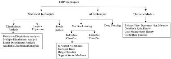
Figure 1.
FDP models.
2.1. Statistical Models for Financial Distress Prediction
Statistical models include univariate discriminant analysis (UDA), multivariate discriminant analysis (MDA), linear probability model (LPM), logistic regression (LR), probit models, cumulative sums procedures (CUSUM), and partial adjustment processes, among others. These models utilize sensitive financial ratios as inputs to predict a firm’s financial crisis by employing statistical tools and techniques.
Early studies in this field include FitzPatrick’s analysis in 1932, which examined business failure prediction across five phases (Fitzpatrick, 1932; Gilbert et al., 1990). Beaver’s work in 1966 associated mean values of 30 ratios with equal number of bankrupt and non-bankrupt companies. Beaver highlighted the predictive power of multiple ratios compared to a single ratio and laid the foundation for bankruptcy prediction models (Beaver, 1966). Altman improved on Beaver’s univariate model by incorporating more ratios and using MDA for bankruptcy prediction (Altman, 1968; Altman et al., 2017). Linear Discriminant Analysis (LDA) is a classification and dimensionality reduction model that follows a linear approach. It was initially developed by Fisher in 1936 for two classes and later extended to multiple classes by C.R Rao in 1948 (Rao, 1948; Shumway, 2001). Quadratic Discriminant Analysis (QDA) is similar to LDA but relaxes the assumption that all classes have equal means and covariances. Ohlson introduced a logistic regression-based model (Ohlson, 1980; Rao, 1948), while Zmijewski addressed sampling bias and oversampling by suggesting the use of probit analysis (Zmijewski, 1984). LR estimates probabilities using logistic functions to examine the relationship between dependent variable and independent variable. The LR algorithm calculates the coefficients from training data using maximum likelihood estimation (Heinze & Schemper, 2002; Zizi et al., 2020). Other notable studies include (Altman et al., 1977; Gilbert et al., 1990; Odom & Sharda, 1990; Pranowo et al., 2010), who explored logistical regression and Artificial Neural Networks (ANN), respectively. Kahya et al. introduced the CUSUM model (Kahya & Theodossiou, 1999; Keige, 1991), and Laitinen investigated Partial Adjustment Models (Laitinen & Laitinen, 1998; Mselmi et al., 2017). Altman proposed the Z- Score and ZETA models (Alfaro et al., 2008; Altman, 2013), while Shumway developed a hazard model (Shumway, 2001; Svetnik et al., 2003). Altman et al. re-evaluated the Z-Score model with additional variables and found it performed well internationally (Altman et al., 2017; Arlot & Celisse, 2010).
However, most of the ratios used in earlier studies depict the following aspects of a business: Profitability, Efficiency, Long-term solvency and Liquidity. Overall, past research has confirmed the predictive power of traditional models, especially when updated with new variables or coefficients. However, the definition of financial distress and the assessment of stress magnitude remain understudied areas, and industry-specific models can be developed to improve bankruptcy prediction.
2.2. Artificial Intelligence Models for Financial Distress Prediction
The evolution of machine learning in FDP began with the introduction of artificial intelligence algorithms, including neural networks and Genetic Algorithms (GA), in the 1990s. Researchers such as Odom et al. and Tam et al. demonstrated the superior performance of AI expert systems compared to traditional statistical methods like logistic analysis during this period (Odom & Sharda, 1990; Pranowo et al., 2010; Tam & Kiang, 1992; Valaskova et al., 2018).
Neural Networks (NNs) methods, in particular, have shown promising results in predicting financial crisis. Aydin et al. suggested their potential for identifying significant patterns in financial variables, highlighting the capacity of these methods to capture complex relationships (Aydin & Cavdar, 2015). The limitations associated with traditional statistical models, including issues of linearity and stringent assumptions, have driven a transition toward machine learning models. These newer models are designed to handle large datasets without requiring strict distribution assumptions, reflecting a more flexible and powerful approach to FDP.
For example, Malakauskas et al. demonstrated that Random Forests (RF), enhanced with time factors and credit history variables, achieved superior accuracy over static-period predictors, indicating the importance of dynamic multi-period modelling (Malakauskas & Lakštutienė, 2021). Jiang et al. emphasized the effectiveness of TreeNet for FDP, achieving over 93% accuracy and showcasing the value of integrating diverse financial and macroeconomic variables, along with non-traditional factors like executive compensation and corporate governance (Jiang & Jones, 2018).
Liang et al. highlighted the critical role of feature selection, showing that the choice of filter and wrapper-based methods could significantly impact prediction accuracy, depending on the underlying classification techniques (Liang et al., 2015). Similarly, Tsai et al. demonstrated that combining clustering methods, such as Self-Organizing Maps (SOMs), with classifier ensembles outperformed single classifiers in predicting financial distress. These findings underline the effectiveness of hybrid models and the synergy between dimensionality reduction and ensemble techniques for enhancing predictive performance (Tsai, 2014).
Overall, the collective findings suggest that while traditional models offer foundational insights, modern machine learning methods bring a greater capacity to manage high-dimensional data, capture nonlinear relationships, and integrate both financial and non-financial predictors. This evolution reflects a significant shift toward more robust and nuanced approaches in FDP, leveraging advanced algorithms and innovative methodologies to improve accuracy and reduce uncertainty in financial decision-making.
2.2.1. Individual Classifier
Within the realm of machine learning, there exists a wide array of single classification algorithms, each designed to tackle specific challenges and inherent patterns within datasets. In the context of this research, we have employed fundamental classifiers that have been instrumental in shaping the landscape of machine learning. This investigation centres on a core set of methodologies that have undergone thorough study and widespread application across diverse domains. These methodologies include k-Nearest Neighbours (KNN), Decision Trees (DT), Ridge Classifier (Ridge) and Support Vector Machines (SVM). KNN algorithm compares new data with previously observed nearest neighbor training data samples using supervised learning approach. It is a straightforward algorithm that classifies cases based on similarity, often utilizing distance functions. The parameter ‘k’ represents the number of closest neighbors considered in the majority vote. KNN is also known as a lazy learning algorithm because algorithm delays the process of generalizing or learning from the training data until a new query instance needs to be classified (Bansal et al., 2022; Faris et al., 2020; Guo et al., 2003; Liang et al., 2018). DT are predictive models that employ a hierarchical or tree-like structure to make decisions about the affiliation of values to classes or numerical target values (Faris et al., 2020; Liang et al., 2018). Ridge Classifier converts label data to the range [−1, 1] using ridge regression method and solves the problem. The highest predicted value is taken as the target class, and multi-output regression is applied to multiclass data (Jones et al., 2017). SVM aims at finding an optimal hyperplane that maximize the class margin. This is achieved by considering the values at the closest distance. SVM utilizes support vectors and boundaries to identify hyperplanes (Hsu & Lin, 2002; Sun et al., 2021). It constructs hyperplanes in high-dimensional or infinite space, making it applicable for regression, classification, and other tasks. SVM allows control over capacity and transformability during model training, making it widely used and effective technique in machine learning (Barboza et al., 2017; Cortes & Vapnik, 1995; Devi & Radhika, 2018; Liang et al., 2018).
To sum up, the evaluation of separate classifiers highlights the importance of selecting models carefully so that they match the unique characteristics of financial data and the specific requirements of distress prediction tasks. The trend for future advancements in prediction skills is the combination of transfer learning and ensemble learning approaches. These encouraging avenues could improve machine learning models’ overall efficacy and flexibility in handling the ever-changing problems associated with FDP. The investigation and application of these cutting-edge methods will probably lead to more reliable and accurate forecasts in the field of FDP.
2.2.2. Ensemble Classifier
Recent studies have explored building ensemble models using single classifier-based AI models (Barboza et al., 2017; Devi & Radhika, 2018; Faris et al., 2020; Huang & Yen, 2019; Liang et al., 2018; Nazareth & Reddy, 2023; Qu et al., 2019; Tsai et al., 2021). Ensemble models, which leverage the collective intelligence of multiple classifiers, have gained prominence for enhancing predictive performance in this context. These models are classified as homogeneous and heterogeneous ensembles, based on whether the constituent base models are of the same or different types (Figure 2). Two key approaches to combining predictions within ensembles are sequential and parallel.
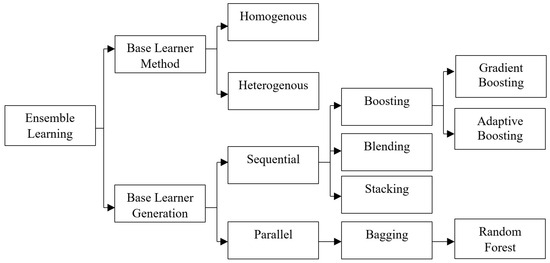
Figure 2.
Classification of ensemble learning.
Sequential ensembles, also known as cascading ensembles, involve training and applying base models in a step-by-step manner, where each model’s output serves as input for the next. This approach is advantageous for capturing complex relationships and offers interpretability, as each model’s contribution can be analysed sequentially. However, weaknesses in early models may propagate through the sequence. In contrast, parallel ensembles, or concurrent ensembles, have independently trained base models. This independence allows for diverse learning and capturing various patterns in the data. The predictions of individual models are aggregated to obtain the final output, with aggregation techniques such as averaging or voting. Parallel ensemble models, with their ability to leverage diverse perspectives, offer a potent framework for improving predictive performance in FDP. Among the frequently used ensemble classification techniques are RF, AdaBoost (ADA), bagging, gradient boosting (GBC), and random subspace (Ho, 1995). RF is a versatile model used for both classification and regression problems in machine learning (Breiman, 2001). It is an ensemble learning method based on the concept of “learning from data”. The core idea of the RF algorithm is to construct multiple decision trees (Tam & Kiang, 1992). RF combines the predictions of these trees to make final predictions. Generally, RF produces more robust and accurate models (Laitinen & Laitinen, 1998). AdaBoost is a boosting method commonly used as an ensemble technique in machine learning (Zhu et al., 2009). It is also referred to as adaptive boosting since it assigns weights to each instance and assigns higher weights to misclassified instances (Alfaro et al., 2008). Gradient Boosting is a boosting algorithm used for high-performance estimation with large datasets. It combines the calculations of multiple basic estimators to enhance robustness compared to using a single estimator (Assaad et al., 2008; Faris et al., 2020; Ho, 1995; Xu et al., 2014). Bagging classifier (Bagging) is a meta-estimator ensemble method that fits base classifiers to random subsets of the original dataset and aggregates their predictions to generate the final prediction. Bagging helps reduce the variance of unstable classifiers, which includes algorithms like DT known for their high variance and low bias. Therefore, utilizing a bagging classifier can be beneficial when working with algorithms such as DT and Variance, RF etc., (Barboza et al., 2017; Breiman, 1996; Faris et al., 2020; Liang et al., 2018). By taking random samples from the training data set, the Bagging approach creates sample subsets that are subsequently used to train the fundamental integration models. In the Bagging model, basic model training is carried out parallelly. The Bagging model is used to reduce variance, improve generalization and mitigate overfitting.
Voting mechanisms play a crucial role in parallel ensemble models, determining how individual base models’ predictions contribute to the final output. Common voting mechanisms in FDP include hard voting (Figure 3a), where a majority vote decides the predicted financial state, and soft voting (Figure 3b), which involves averaging predicted probabilities for a more nuanced prediction. Weighted voting assigns different weights to base models based on reliability or historical performance. Stacking involves training a meta-model that learns to combine predictions, allowing for more complex interactions between models. Hard voting is the most suitable ensemble method when using diversified baseline classifiers, because it offers an optimal balance between performance, simplicity, and compatibility. Unlike soft voting, which requires calibrated probability estimates and additional steps for models like Ridge Classifier and SVM, hard voting integrates all classifiers without modification. Compared to stacking, which introduces higher complexity and computational overhead, hard voting remains efficient, interpretable, and less prone to overfitting. Even if soft voting and stacking may yield marginal accuracy improvements, their added complexity and calibration requirements often outweigh their benefits. Thus, hard voting provides consistent, stable performance across diverse algorithms with minimal risk and overhead, making it the most practical and effective choice for this financial distress prediction framework. Ultimately, the choice between sequential and parallel ensembles, as well as the specific voting mechanism employed, depends on factors such as the nature of dataset, task complexity, and the desired balance between interpretability and computational efficiency.
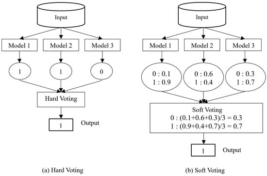
Figure 3.
Types of voting mechanism (a) Hard voting (b) Soft Voting.
While parallel ensembles are computationally efficient and less susceptible to error propagation, they may struggle with capturing intricate dependencies or sequential patterns, and interpretability can be challenging. Hence, building an optimal ensemble classifier for FDP requires addressing three main challenges: selecting the best classification method, determining the number of classifiers for the ensemble, and choosing a binding method to combine the individual classifiers’ outputs (Figure 4). To address these challenges different combinations of baseline classifiers for improved performance. Studies have shown that combining a set of classifiers yield higher predictive rates than using individual classifiers alone (Abellan & Castellano, 2017; Ala’raj & Abbod, 2016).
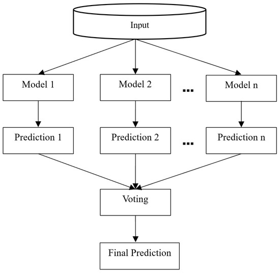
Figure 4.
Structure of ensemble model (Bagging).
Ensemble approaches offer a number of benefits, including increased flexibility in the model selection process, increased accuracy compared to single models by combining the best features of multiple models (Abellan & Castellano, 2017; Ala’raj & Abbod, 2016), increased resilience to noise and outliers in the data due to their consideration of multiple perspectives, and a reduction in overfitting in complex models by generalising patterns discovered from various data subsets. Both statistical and AI models have been extensively studied, confirming their predictive power and potential for improving decision making (Nazareth & Reddy, 2023). However, further research is needed to explore the definition and measurement of financial distress, as well as the development of industry-specific models. The use of ensemble techniques and optimal ensemble classifiers holds promise for enhancing prediction accuracy.
2.2.3. Theoretical Models for Financial Distress Prediction
FDP has been explored through various theoretical models, each offering unique perspectives on the factors leading to corporate failure. Below are the key models in financial and economic theory:
Balance Sheet Decomposition Measures (BSDM) and Entropy Theory: This method is used to predict financial distress by analyzing shifts in a firm’s balance sheet structure. This approach is based on the concept that firms strive to maintain equilibrium in their financial structure, with a balanced composition of assets and liabilities. Significant deviations from this balance, indicated by increased entropy or disorder in the financial statements, suggest a breakdown in financial stability. Such changes may signal that a firm is at risk of financial distress, making this approach useful for early detection of financial instability (Booth, 1983; Lev, 1973; Theil, 1969).
Gambler’s Ruin Theory: This theory models a firm’s financial survival by comparing it to a gambler who continues playing until they run out of money. According to this theory, a firm operates with a certain probability of financial gain or loss each period. If the firm experiences a prolonged sequence of negative cash flows, it will eventually deplete its capital, leading to bankruptcy. The probability of bankruptcy increases with the duration of financial losses and the initial capital available to the firm. This theory is particularly useful for assessing long-term financial sustainability under conditions of uncertainty and volatility (Morris, 2018; Scott, 1981).
Cash Management Theory: This theory focuses on the importance of effectively managing a firm’s short-term cash flows to avoid financial distress. According to this theory, firms must maintain a balance between cash inflows and outflows to ensure liquidity. Persistent imbalances, where cash outflows consistently exceed inflows, indicate poor cash management, which can lead to liquidity problems and eventually bankruptcy. Effective cash management is therefore crucial for maintaining financial stability and preventing financial distress, especially in firms with highly variable cash flows (Aziz et al., 2013; Laitinen & Laitinen, 1998).
Credit Risk Theories: These theories are a set of approaches used to assess the likelihood of a borrower defaulting on their financial obligations, primarily in the context of financial institutions. These theories underpin several key models, including JP Morgan’s CreditMetrics, Moody’s KMV model, CSFB’s CreditRisk+, and McKinsey’s CreditPortfolio View, each of which evaluates credit risk using different methodologies.
JP Morgan’s CreditMetrics and Moody’s KMV models rely on option pricing theory, where a firm is considered to be in default if the value of its assets falls below its liabilities, with default being an endogenous outcome related to the firm’s capital structure (Black & Scholes, 1973; Merton, 1971).
CSFB’s CreditRisk+ applies an actuarial approach, using a Poisson process to model default events and derive the loss distribution of a credit portfolio (Credit Suisse, 1997).
McKinsey’s CreditPortfolio View incorporates macroeconomic factors such as interest rates, GDP growth, and unemployment rates into the assessment of credit risk, linking the probability of default to broader economic conditions (Wilson, 1998).
2.3. Hyper Parameter Tuning
Optimizing hyperparameters is a pivotal stage in the development of high-performing machine learning models, particularly when applied to predicting financial distress. This process involves fine-tuning configuration settings, referred to as hyperparameters, to achieve optimal model performance. Various methods, ranging from traditional approaches like Grid Search (GS), Random Search (RS), and Gradient Descent, to advanced techniques such as Bayesian Optimization (BO) and Nature-Inspired Heuristic Algorithms, are employed to enhance accuracy, efficiency, and generalization across diverse financial datasets. Decision-theoretic methods, a fundamental approach in hyperparameter tuning, entail defining a hyperparameter search space and identifying the most effective combinations within that space. Grid Search, a decision-theoretic method, conducts an exhaustive search, but computational time escalates significantly with an increased number of hyperparameters (Bergstra et al., 2011; Kartini et al., 2021). Random Search serves as a valuable alternative, introducing randomness by employing arbitrary combinations, thereby gaining independence from the number of hyperparameters (Bergstra & Bengio, 2012). However, Random Search’s major limitation lies in its high dependence on randomness, resulting in varied outcomes for different parameter sets (Jerrell, 1988). Unlike GS and RS, BO models make use of past hyperparameter evaluations to inform the selection of the next hyperparameter values, reducing unnecessary evaluations and accelerating the detection of optimal combinations within fewer iterations (Eggensperger et al., 2013). Researchers have also explored nature-inspired methods for efficient hyperparameter optimization in the context of FDP. Han et al., conducted a survey on metaheuristic algorithms for training random single-hidden layer feedforward neural networks (RSLFN) (Han et al., 2019), while Khalid et al. reviewed both nature-inspired and statistical methods for tuning the hyperparameters of SVM, NNs, Bayesian Networks (BNs), and their variants (Khalid & Javaid, 2020).
In FDP, the careful optimization of hyperparameters is crucial for obtaining accurate and reliable model predictions. Researchers and practitioners in this domain can benefit from exploring a range of hyperparameter tuning methods, considering the specific nature of financial data and the intricacies of predicting distress in financial contexts.
The study by Barboza et al. assesses how well SVM, bagging, boosting, RF, and other machine learning models predict corporate bankruptcy one year ahead of time (Barboza et al., 2017). These models are contrasted in the study with more conventional statistical techniques like LR, discriminant analysis, and NNs. In order to increase prediction accuracy, the research uses data on North American firms from 1985 to 2013 along with additional financial indicators. Notably, adding new variables to machine learning models improves accuracy significantly; RF model outperforms the others, scoring 87% as opposed to 50% for LDA and 69% for LR. The accuracy of machine learning models—RF in particular—is about 10% higher than that of conventional statistical methods. The disadvantage is the computational time needed by some machine learning models, like SVM.
The significance of anticipating financial distress in customer loans within financial institutions is discussed in a 2018 study by (Liang et al., 2018). This study focuses on improving the prediction accuracy and minimizing Type I errors, which incur substantial costs for financial institutions through Unanimous Voting (UV) which predicts Bankruptcy even if one classifier declare bankruptcy out of ‘N’ classifiers. The UV ensemble mechanism resulted in better performance than the ensemble methods such as bagging and boosting and also yielded good results than the single classifiers (SVM, CART, KNN, MLP, Bayes) when applied on varied datasets. The limitation of this Unanimous Voting mechanism is that this automatically avoids Type-I error unless all the N classifier predicts wrongly. This leads to increase in Type-II error.
The review by Devi and Radhika in 2018 shows the importance of Machine learning approaches such as ANN, SVM and DT over the traditional statistical methods such as LDA, MDA and LR (Devi & Radhika, 2018). The review results shows that SVM model optimized with Particle Swarm Optimization (PSO) have achieved higher results of (95% accuracy and 94.73% precision). The study concludes that machine learning model integrated with the optimization algorithms will improve the accuracy and suggests future directions for exploring the evolutionary techniques for improvements in financial risk assessment. But this study failed to present the merits and demerits of the reviewed models.
The review by Qu et al. (2019) states the current advancements in bankruptcy prediction and explore potential innovations and future trends in this field, particularly through machine learning and deep learning techniques (Qu et al., 2019). One significant trend is the diversification of data sources. Traditionally, bankruptcy prediction models rely on numerical data such as financial statements and accounting records. However, this review highlights incorporating textual data from sources like news articles, public reports and expert commentary using deep learning techniques. This shift has introduced the concept of Multiple-Source Heterogeneous Data, which integrates both structured and unstructured information for more comprehensive analysis. Deep learning techniques, such as Convolutional Neural Networks (CNNs) are used to effectively process and classify such complex data.
Huang and Yen (2019) explores the performance of various machine learning algorithms in predicting financial distress using data from Taiwanese firms (2010–2016) and 16 financial variables. The work performs comparison on four supervised machine learning models such as SVM, HACT, Hybrid GA-fuzzy clustering and XGBoost against a DBN which is an unsupervised model and a Hybrid DBN-SVM model. Their results shows that XGBoost gives the best performance among the supervised methods whereas the hybrid DBN-SVM model outperforms both standalone SVM and DBN. The advantage of integrating unsupervised feature extraction with supervised learning has been highlighted over traditional methods and stressed the importance of hybrid models in improving predictive performance.
The analysis done by Faris et al. (2020) tackles the problem of imbalanced datasets with 478 Spanish companies for a period of six years (with only 62 bankruptcies). The class imbalance is addressed by applying SMOTE and evaluation is carried out using five different feature selection methods. The model is tested on both baseline classifiers and ensemble models. The authors’ study results show that SMOTE with AdaBoost achieves the highest accuracy of 98.3% and the lowest Type I error as 0.6%.
The study done by Tsai et al. (2021) explores the possible combinations of different feature selection and instance selection with ensemble classifier to analyse the financial distress and give a useful insight to the investors. This study was carried out on ten different datasets which amounts to 288 experiments. The authors claim that the order of preprocessing enhances the performance but the preprocessed data is not tested on the same classifiers and hence the suitability of the preprocessing technique is unclear. The preprocessing is carried out by combining optimal t-test-SOM with bagging DT for AUC and PCA-AP with ANN which minimizes type II errors.
The literature review underscores the pivotal role played by both statistical models and AI in the realm of FDP. It stresses the ongoing necessity for research aimed at refining financial distress classifications and metrics. Notably, optimal ensemble classifiers and ensemble techniques are recognized as valuable strategies capable of substantially enhancing prediction accuracy in this domain. The incorporation of these advancements is deemed essential for improving the effectiveness of predictive models by tuning the hyperparameters, acknowledging the dynamic and critical nature inherent in financial crisis prediction. This synthesis of statistical and AI approaches stands as a key step towards more robust and reliable predictions in the field of financial distress.
3. Empirical Experiment
In this study, a practical examination was carried out to assess the efficiency of the proposed methodology. Data obtained from automobile companies in India were utilized for this purpose. This section presents comprehensive information on the process of data collection, pre-processing of the data, the experimental design, and the subsequent analysis of the empirical results.
3.1. Data Collection
3.1.1. Dataset
The sample of firms was derived from the corporate database ProwessIQ maintained by the Centre for Monitoring Indian Economy (CMIE). This study was conducted for automobile manufacturing companies in India whose year of incorporation is after the 1950s. Firms that underwent mergers or diversification were excluded to ensure data consistency and comparability, as such events alter financial structures and risk profiles, making pre- and post-event metrics incomparable. This exclusion also mitigates survivorship bias, as these firms may have strategically avoided financial distress. Seven years of financial data were taken for this study. All years’ financial information’s extracted from financial statements and cash flow statements of the companies. Companies’ profit and loss statement for seven years period (2013–2019) is identified from the Auditor’s report which is released along with the annual report of the companies after the audit every year.
In this study, companies with seven consecutive years of profitability are categorized as “healthy”, while those with seven consecutive years of losses are classified as “distressed”. From the dataset we identified 50 companies classified as loss making and 380 companies as profit-making. The pairing of loss and a profit-making company is determined based on the asset size of the companies following the methodology outlined by (Beaver, 1966; Gilbert et al., 1990). A paired sample of fifty companies each from both groups has been selected for further analysis. For the dependent variable Y, the Healthy company is denoted as 1, and the distressed company is denoted as 0. Ratios have been categorized to identify the loss or profitability of the company and are normalized.
3.1.2. Feature Selection
Beaver has previously demonstrated the predictive potential of financial ratios in forecasting financial distress (Beaver, 1966). In this study, a comprehensive dataset comprising of 78 ratios was collected. The selection of these financial ratios as initial features for the FDP model was based on their ability to predict and differentiate between healthy and distressed firms. Specifically, 23 variables were chosen for predicting financial distress based on their extensive utilization in previous research, as is evident in the studies (Chen & Shimerda, 1981; Jabeur, 2017; Kliestik et al., 2020; Kovacova et al., 2019; Laitinen & Laitinen, 1998; Ohlson, 1980; Pedregosa et al., 2011; Wu et al., 2020; Zmijewski, 1984). Consequently, these variables were deemed suitable for this experiment.
Ultimately, 23 feature variables (Table 1) were chosen in such a way that it covers the major four categories: Profitability, Liquidity, Leverage/Solvency, and Turnover/Activity/ Efficiency Ratio 1. The profitability ratio evaluates the effectiveness of management in utilizing business resources to generate profits. A company with higher profitability is more capable of fulfilling its debt obligations and avoiding financial distress. Xu et al. suggested that companies with higher profitability are less likely to experience financial distress (Xu et al., 2014; Yim & Mitchell, 2005). 2. The liquidity ratio measures a firm’s ability to meet its short-term obligations. A higher ratio indicates that the company possesses more short-term assets than short-term liabilities. Study by Altman et al. indicates that liquidity ratios play a crucial role in predicting financial distress (Altman, 1968). It is recommended that companies maintain sufficient liquidity to prevent insolvency issues. Additionally, higher liquidity enables companies to meet their financial obligations promptly (Kiragu, 1991). Similar studies by Kiragu and Ohlson demonstrate that the current asset to current liabilities ratio successfully predicts bankruptcy (Kiragu, 1991; Kisman & Krisandi, 2019; Ohlson, 1980; Rao, 1948). 3. The leverage/solvency ratio assesses a business’s ability to sustain itself over the long term. This ratio can be divided into the debt ratio and the debt- to-equity ratio. Higher leverage, characterized by higher total debt and a lack of cash flow, is associated with company bankruptcy. Paranowo finds that leverage ratios represented by debt service coverage are significant predictors (Salcedo-Sanz et al., 2014). Keige also concludes that the leverage ratio is a significant predictor of corporate distress (Keige, 1991). 4. The turnover/activity/efficiency ratio measures a firm’s efficiency in generating revenue by converting production into cash or sales. A higher turnover ratio indicates better utilization of assets, reflecting improved efficiency and profitability. These ratios provide insights into a company’s performance strengths and weaknesses. To remain competitive in the marketplace, companies can take additional measures to ensure the effectiveness of their activities.

Table 1.
Variables used in the prediction model.
3.2. Data Pre-Processing
Data pre-processing is a valuable technique used to enhance the quality of data and achieve normalization within a dataset, aiming to rectify errors like outliers and eliminate redundant information. Maintaining data integrity is of utmost importance in this study, necessitating organizations to possess a minimum historical record spanning three years prior to and during the data collection period. Some distressed organizations exhibited missing values, requiring a thorough examination of these cases and an assessment of data availability. Companies with a significant number of missing values were excluded from the study. As a matched pair approach was utilized, removing a company from the distressed sample led to the exclusion of its corresponding healthy firm variables, and vice versa. The pre-processing phase includes by loading the dataset and inspecting the presence of numeric values, while non-numeric attributes or data were discarded. Numeric data was deemed preferable for processing and predicting financial distress. Consequently, the dataset was loaded with refined numeric values.
The Firm-Feature-Wise three-step Missing Value Imputation Algorithm 1 is designed to handle missing values in time-series financial data for multiple firms. It employs a systematic approach to impute missing values based on their position in the time series. This approach consists of three steps: (1) The algorithm employs backward fill for missing data in the first year, substituting the data from the following year for the missing value. In the event that the data for the following year is also missing, mean imputation (1) is used, which uses the firm’s average feature value for all years. (2) Similar to this, the algorithm employs forward fill for missing data in the last year, substituting the missing value with data from the previous year. If the data from the prior year is not available, mean imputation (1) is used. (3) For missing data in the middle years, the algorithm computes the missing ratio for each feature and uses mean imputation (1) only if less than half of the data for that feature is missing. This ensures that the imputed values are representative of the firm’s historical data while avoiding biases from other firms or features. The algorithm is firm-specific, preserving the unique characteristics of each firm’s financial data, and is scalable to handle large datasets with multiple firms, years, and features.
where:
- is the mean of feature f for firm i.
- represents the set of years for which the feature f is observed (i.e., non-missing values).
- is the observed value of feature f for firm i at year t.
- is the total number of observed years for feature f in firm i.
| Algorithm 1 Firm-Feature-Wise three step imputation process. |
|
Descriptive statistics, such as kurtosis and skewness, were employed to evaluate the characteristics and nature of the data following the imputation process, with a particular emphasis on assessing the level of normal distribution. The normalization process was carried out using Equation (2):
After outlier and normalization treatment, OLS test is used to check the predicting ability of the dataset. The OLS result (Table 2) shows that Jarque-Bera probability value is 0.000128 which is <0.05 i.e., this dataset has the capacity for prediction (Thadewald & Büning, 2007).
Table 2.
Result of OLS Regression model.
3.3. Design of Empirical Experiment
3.3.1. Design of Experimental Process
The experimental process is designed to systematically evaluate and compare the performance of various classification techniques for FDP. Our objective is to incorporate a diverse set of classifiers that represent distinct algorithmic paradigms, enabling a comprehensive and balanced performance comparison. The selected 11 baseline classifiers encompass a broad methodological spectrum: (i) Linear Models—LR, RIDGE and LDA; (ii) Non-linear Models—KNN, QDA, SVM, and DT; (iii) Ensemble Methods—Bagging, RF, ADA, and GBC. This diversity allows us to evaluate the performance of our proposed method across a wide range of modeling paradigms, from simple linear models to complex ensemble methods. An odd number of baseline models are selected to avoid ties in the voting mechanism. After preprocessing, the dataset is split into training and testing sets using a 70:30 ratio. The training set is used to build and fine-tune the models, while the test set is reserved for evaluating the final performance of the models. This ensures that the performance metrics reflect the models’ ability to generalize to unseen data.
This study consists of four sets of experiments. Figure 5 shows that the initial experiment involved training and testing each of the eleven baseline algorithms individually. By combining different algorithms, we can leverage their diverse strengths and compensate for individual weaknesses. This often results in a more robust and accurate predictive model. Hard voting mechanism allows each model in the ensemble to vote for a class and the class that receives the majority of votes is the final prediction. This is suitable when the individual models provide discrete class prediction which helps in reducing error. So, the second experiment entailed training and testing using a combination of all eleven baseline algorithms. The combination of the eleven algorithms results in a total of 2048 combinations. However, one of these combinations is found to be empty and thus not useful. Consequently, 2047 combinations of algorithms are utilized for this study. All 2047 combinations are inputted into HVM, and their performance is evaluated.
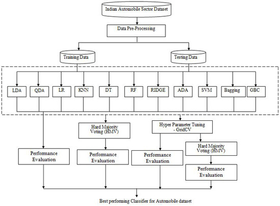
Figure 5.
Schematic diagram showing the experimental design.
The performance and behavior of machine learning algorithms are often significantly impacted by the values of hyperparameters. Thus, the third experiment is carried out to identify optimized hyperparameters for all baseline algorithms using GridSearchCV. This involves finding the best parameter configuration for each model, and subsequently evaluating the performance of the individual baseline models with the test data. Similarly, in the fourth experiment, the combination of baseline models is examined, but this time with the inclusion of optimized hyper parameters for each algorithm. Finally, k-fold CV is used to assess the generalizing ability of the prediction model.
3.3.2. Crosss-Validation (CV)
The primary objective when developing classification or regression models is to ensure their ability to generalize. It is crucial to evaluate the model’s performance using data that was not used for training, as relying solely on the training data may lead to biased results, especially when dealing with limited datasets. Even if a model performs well when trained and tested on a small portion of the data, there is a possibility of achieving even better results when trained on the entire dataset.
To address this issue, a commonly employed technique known as k- fold CV is utilized in classification and regression models (Bergmeir & Benítez, 2012; Odom & Sharda, 1990; Stone, 1974). The validation process is repeated k times, with each iteration using a different fold as the validation set (Figure 6). This approach provides an estimation of the validation error for each iteration, which is then averaged to obtain the final validation error. By repeatedly performing the validation process, k-fold CV offers greater robustness compared to the validation set approach. Therefore, k-fold CV is employed to validate the model’s performance.
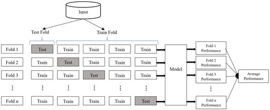
Figure 6.
k-fold Cross-Validation.
3.3.3. Hyperparameter Tuning with GridSearchCV
Objective functions and constraints are crucial components in computing optimization algorithms. Grid search is a fundamental method for hyperparameter optimization (HPO), conducting an exhaustive search on user-specified hyperparameter sets. It is applicable for hyperparameters with a limited search space, and its straightforward nature leads to accurate predictions. Despite suffering from the curse of dimensionality, grid search remains widely used due to its simplicity, ease of parallelization, and flexibility in resource allocation (Bergstra & Bengio, 2012).
Hyperparameter tuning with GridSearchCV optimizes machine learning models by combining the exhaustive search of grid search with Cross-Validation (Figure 7). It identifies optimal hyperparameter values from the given set of user-specified hyperparameter, enhancing model accuracy and generalization.
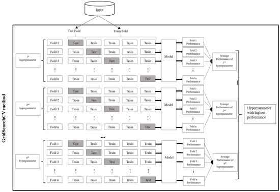
Figure 7.
Hyperparameter tuning using GridSearchCV method.
3.3.4. Model Evaluation Measure
In this study on FDP with matching pair dataset using machine learning models, Accuracy (3) is primarily used as an evaluation measure of the model. Apart from accuracy, most of the common evaluation measures for the classification models, namely Precision (4), Recall/Sensitivity (5), Specificity (6), Type-I error (8), Type-II error (9), F1 score (10), and AUC ROC curve where adopted. For classification problems, most of the performance evaluation measures are calculated using the confusion matrix, but the matrix itself is not the performance measure. Table 3 shows the structure of a confusion matrix.
Table 3.
Confusion Matrix.
Two-class classification problem focusing on FDP has been employed in this work. The two classes are labelled as Distress (Class 0) and Non-Distress (Class 1). When dealing with a two-class problem, the confusion matrix provides four possible combinations of actual and predicted values. True Positive (TP), False Positive (FP), False Negative (FN) and True Negative (TN).
The F1 score, also known as the F score (10), is a commonly used metric to evaluate the performance of binary classification models. Its main purpose is to compare the effectiveness of two learning classifiers. For example, if classifier A has a high recall rate while classifier B has a high precision rate, the F1 scores of both classifiers can be utilized to determine which one produces better outcomes. The F1 score ranges between 0 and 1, where a lower F1 score indicates reduced sensitivity of the model. Conversely, when both precision and recall scores are high, a higher F1 score suggests that the model possesses greater sensitivity.
The AUC refers to the measurement of the ROC curve. The AUC ROC quantifies the effectiveness of a classifier in accurately distinguishing positive classes from negative classes. A higher AUC value indicates that the classifier is more proficient in correctly identifying distressed firms as distressed and healthy firms as healthy.
4. Experimental Result and Analysis
4.1. Performance of Individual Baseline Classifiers
The initial experiment aimed to assess the performance of each individual baseline classifier. All 11 baseline models were trained and evaluated using the same dataset. The performance of the individual baseline classifiers, including accuracy, AUC-ROC, confusion matrix, and error rate, is presented in Table 4. Among the 11 classifiers, GBC (Gradient Boosting) exhibited the highest accuracy of 0.99048. It is important to note that since this study utilized a matching paired samples dataset, if a model achieves higher accuracy, the remaining evaluation metrics tend to yield similarly favourable scores for that model. The AUC-ROC score for the GBC model was 0.9900, and the error rate was 0.010. These results were obtained without hyperparameter tuning.
Table 4.
Results of individual Baseline algorithms.
4.2. Performance of Individual Baseline Classifiers After Hyperparameter Tuning
Parameter tuning is considered one of the most effective approaches to enhance model performance. By fine-tuning the parameters, the prediction accuracy of a model can be significantly improved. The process of manually adjusting parameters can be time-consuming and resource-intensive, making it impractical. To overcome this challenge, the GridSearchCV technique is employed to automate the fine-tuning of hyperparameters.
GridSearchCV is a method that systematically explores a predefined set of parameter combinations to find the optimal values. It searches for the best parameter values based on a specified scoring metric such as accuracy, F1 score (Shilpa & Amulya, 2017). The GridSearchCV technique generates the best combination of parameters that yield the highest accuracy value. These parameters obtained through GridSearchCV are then utilized in the 11 baseline models, which are individually tested after hyperparameter tuning.
Table 5 shows the performance of the individual classifier with the tuned optimal hyperparameters. After tuning, the performance of the LR, KNN, DT, RF, RIDGE, and SVM classifiers algorithms improve in predicting a company’s financial distress situation at 0.94286, 0.96667, 0.96667, 0.98095, 0.91429 and 0.96667 respectively. After hyperparameter tuning also GBC (Gradient Boosting) is showing superior to other baseline classifiers with an accuracy of 0.99048.
Table 5.
Results of individual Baseline algorithms after hyperparameter tuning.
Figure 8 shows the accuracy of the baseline algorithms before and after hyperparameter tuning. The analysis demonstrates that the LR and SVM models exhibited significant improvement in performance following hyperparameter tuning. However, certain models such as LDA, QDA, ADA, Bagging, and GBC attained optimal results with their default parameter settings, indicating no enhancement in predictive accuracy. Notably, the GBC model outperformed all other models, achieving an impressive accuracy of 0.99048.
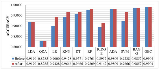
Figure 8.
Accuracy performance comparison between baseline algorithms before and after hyperparameter tuning.
4.3. Performance of HVM Algorithms with the Combination of the Baseline Algorithm Without Hyperparameter Tuning
As mentioned earlier in the experimental process design (see Section 3.3.1), experiments were performed on all 2047 combinatorial models using an HVM without hyperparameter tuning. The results obtained show these six algorithms (Bagging, GBC, RF, LDA, KNN, and ADA (BGRLKA)) played a major role in prediction with lower error rates. Bagging reduces variance by averaging multiple models trained on different subsets of data. Boosting (AdaBoost, GBC) focuses on sequential learning, where errors are reduced in each iteration. LDA capture linear relationships in the data and non-linear patterns is identified with Random Forest with this KNN helps to capture local decision boundaries. Using an ensemble of BGRLKA algorithms allows us to balance variance, bias, and robustness, higher accuracy and lesser error rate. Ensemble BGRLKA algorithms results in a balanced model leading to better generalization and higher predictive performance. Therefore, combination of BGRLKA algorithms was used as fixed algorithm and remaining 5 algorithms (QDA, LR, DT, RIDGE, and SVM) were treated to all possible combinations to have 32 distinct models
Given the combination of 32 models to the HVM, the result obtained is shown in Table 6, depicte that BGRLKA + QDA combination gives the highest accuracy of 0.99048 with error rate, Type-I and Type-II error as 0.01, 0.009, and 0.01 respectively. The second-best accuracy is 0.9857, and the accuracy of the two models is the same, BGRLKA + LR and BGRLKA + QDA + DT. The accuracy (0.9859) and error rate (0.01) of both algorithms are the same, but the values in the confusion matrix are different and are reflected in the precision, recall, specificity, Type I, and Type II values. If the accuracy is tied, the AUCROC score breaks the tied. BGRLKA + LR model and BGRLKA + QDA + DT model have AUCROC scores of 0.9859 and 0.9855, respectively, so the model with the highest AUCROC score is considered the best. Therefore, the BGRLKA + LR is considered the second-best model for this dataset. Figure 9 shows the performance of each model against its accuracy.
Table 6.
Results of HVM with the 32 combinations of the baseline algorithm.
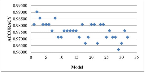
Figure 9.
Results of HVM with the 32 combinations of the baseline algorithm.
4.4. Performance of HVM Algorithms with the Combination of the Baseline Algorithm with Hyperparameter Tuning
The findings indicated that there was no notable enhancement in accuracy when comparing individual baseline classifiers to HVM without tuned hyperparameters. As a result, the hyperparameters of all 11 baseline models were adjusted prior to their combination and utilization in the HVM. The result obtained in (Table 7) shows that BGRLKA + RIDGE + SVM model achieved an accuracy of 0.99524 with 0 for Type-I error and 0.01 for Type-II error. The results show that RIDGE and SVM along with the BGRLKA algorithms play a good role in improving the prediction accuracy. Figure 10 shows the performance of each model after hyperparameter tuning against its accuracy.
Table 7.
Results of HVM with the 32 combinations of the baseline algorithm with tuned hyperparameters.
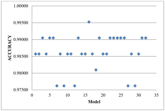
Figure 10.
Results of HVM with the 32 combinations of the baseline algorithm with tuned parameters.
4.5. Performance of HVM Algorithms in k-Fold Cross Validation (k-Fold CV)
To assess the effectiveness of a machine learning model, it is necessary to evaluate its performance using unseen data. The model’s ability to generalize, whether it is under-fitting or over-fitting, can be determined based on its performance on unseen data. The k-fold CV technique is employed to validate the model’s generalizability. We selected k = 5 in CV as a pragmatic balance between bias and variance, particularly suited for datasets of our size and computational resources. With 100 firms and 7 years of data, 5-fold CV ensures that each fold contains a sufficiently representative and diverse sample of companies, allowing robust model evaluation while maintaining computational efficiency during testing across 32 ensemble models.
Regarding the bias-variance trade-off, increasing the number of folds (e.g., k = 10) can reduce the bias of the performance estimate, but at the cost of higher variance and increased computational load, especially when tuning complex ensembles. Conversely, lower k-values (e.g., k = 3) may reduce variance but increase the bias. The choice of k = 5 strikes a balance, minimizing both overfitting risk and computational cost in our high-dimensional setting, without significantly compromising model evaluation accuracy. The purpose of the validation phase in Cross-Validation is to select the best-performing approach and assess the model’s training effectiveness. Table 8 presents the 5-fold CV HVM results for 32 combinations of the baseline algorithm.
Table 8.
Results of 5-fold CV HVM with the 32 combinations of the baseline algorithm.
Figure 11 shows the result of the k-fold CV of the baseline algorithm, BGRLKA and BGRLKA + DT model achieved the best accuracy as 0.97000 with the difference of 0.01095 with our precious baseline algorithm with HVM results. For the model BGRLKA + QDA which got better accuracy of 0.99048 without 5-foldCV, now with 5-fold CV same model got the accuracy of 0.96714 with a difference of 0.02333.
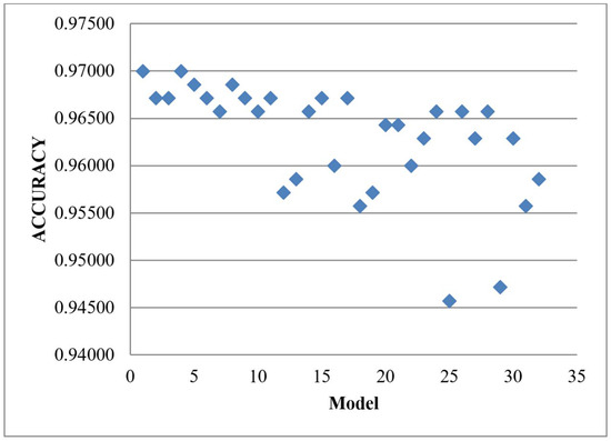
Figure 11.
Results of 5-fold CV HVM with the 32 combinations of the baseline algorithm.
Similarly, Table 9 shows the mean accuracy results of 5-fold CV HVM with the 32 combination of the tuned hyperparameter baseline algorithm. Figure 12 shows BGRLKA + QDA + LR+ DT model achieved the best accuracy as 0.97429 with the acceptable difference of 0.01143 with our precious tuned baseline algorithm with HVM results. For the model BGRLKA + RIDGE + SVM which got better accuracy of 0.99524 after hyperparameter tuning but without 5-fold CV, now with 5-fold CV same model got the accuracy of 0.96000 with the difference of 0.02667. Across 32 model combinations, the average accuracy difference between models evaluated with and without 5-fold cross-validation ranges from 0.00381 to 0.02571 for those without hyperparameter tuning and from 0.00619 to 0.02667 for those with hyperparameter tuning. Similarly, the standard deviation difference ranges from 0.005345 to 0.016660 for models without hyperparameter tuning and from 0.005345 to 0.016288 for models with hyperparameter tuning. These results demonstrate that the algorithm delivers consistent and reliable performance regardless of the specific data used for training and testing. Among the tested combinations, the model comprising BGRLKA + RIDGE + SVM exhibits strong generalization.
Table 9.
Results of 5-fold CV HVM with the 32 combination of the tuned hyperparameter baseline algorithm.
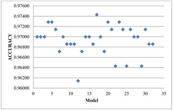
Figure 12.
Results of 5-fold CV HVM with the 32 combination of the tuned hyperparameter baseline algorithm.
In this study we have done the exhaustive search to identify the best model combination that achieves better accuracy with lesser Type-I and Type-II error. Our proposed Firm-Feature-Wise three step imputation process along with HVM of BGRLKA + RIDGE + SVM model combination after tuning, not only achieved a good accuracy of 0.99524 but also achieved lowest error rate (0 for Type-I error and 0.01 for Type-II error). Even for statistical t-test, BGRLKA + Ridge + SVM model had shown significance (p < 0.05) which means that this combination of model still performs better than other models. Additionally, our imputation algorithm addresses a critical preprocessing gap by preserving feature interdependencies during missing data imputation, unlike traditional methods that may distort data distributions (e.g., mean or median imputation, Interpolation, KNN imputation). The findings of this study suggest that the optimal combination of techniques presented can be effectively utilized by financial experts to enhance predictive accuracy, thereby supporting more informed decision-making while minimizing associated risks.
5. Conclusions
The research on FDP has gained significant attention across various disciplines such as accounting, finance, economics, and engineering. This topic has evolved into an independent subject with practical implications for identifying financial risks, preventing financial distress, and avoiding bankruptcy. FDP plays a crucial role in mitigating corporate bankruptcy risks. Previous studies have primarily focused on improving prediction accuracy, with equal emphasis given to reducing Type-I errors to protect stakeholders. While individual classifiers have been extensively researched for FDP, the use of ensemble classifiers in this context is relatively new. Ensemble classifiers overcome the limitations of single classifiers by combining their predictions through specific methods to enhance prediction performance and stability. In this study, an ensemble classifier based on the HVM was employed to achieve high prediction accuracy and minimal Type-I errors. The model was compared with and without hyperparameter tuning, with the results demonstrating that hyperparameter tuning improved accuracy. The best-performing ensemble model not only eliminated Type-I errors but also lowered Type-II error rate which demonstrate high sensitivity and the model’s ability to reliably detect distressed cases. This low-rate highlights that, despite the focus on reducing false positives, the models maintained strong recall and ensured that financially unstable firms were accurately identified. Therefore, the combination of ensemble classifiers using the majority voting mechanism proves to be an effective approach for predicting financial distress in firms. Additionally, the study assessed the model’s generalizability using k-fold CV.
This study focused on the classification of financial distress in Indian automobile manufacturing companies using a paired dataset to identify the most effective model combination. While the findings provide valuable insights, as future work we are extending this study by evaluating model performance on imbalanced datasets and applying it to diverse industries and geographic regions to enhance generalizability. Additionally, incorporating trend analysis to understand the temporal dynamics of financial distress and developing a financial distress forecasting framework will further strengthen the model’s predictive capabilities and real-world applicability.
Author Contributions
Conceptualization, M.M. and N.D.P.S.; methodology, M.M.; software, M.M.; validation, M.M. and N.D.P.S.; formal analysis, M.M. and N.D.P.S.; investigation, M.M. and N.D.P.S.; resources, M.M.; data curation, M.M.; writing—original draft preparation, M.M.; writing—review and editing, M.M. and N.D.P.S.; visualization, M.M.; supervision, N.D.P.S.; project administration, N.D.P.S. All authors have read and agreed to the published version of the manuscript.
Funding
This research received no external funding.
Institutional Review Board Statement
Not applicable.
Informed Consent Statement
Not applicable.
Data Availability Statement
The dataset used in the work is acquired from the corporate database ProwessIQ maintained by the Centre for Monitoring Indian Economy (CMIE). The data is accessed through institutional license under VIT user. The data is used for studying the performance of automobile manufacturing companies in India. Since the data is licensed, access is restricted to authorized users only. CIME ProwessIQ https://prowessiq.cmie.com/.
Acknowledgments
This research is supported by the Department of Science and Technology (DST), India, under the Fund for Improvement of S&T Infrastructure in Universities and Higher Educational Institutions (FIST) Program [Grant No. SR/FST/ET-I/2022/1079], and a matching grant from VIT University. The authors are grateful to DST-FIST and VIT management for their financial support and the resources provided for this work. We thank VIT Business school for providing support to access ProwessIQ database maintained by Centre for Monitoring Indian Economy (CMIE).
Conflicts of Interest
The authors declare no conflicts of interest.
References
- Abellán, J., & Castellano, J. G. (2017). A comparative study on base classifiers in ensemble methods for credit scoring. Expert Systems with Applications, 73, 1–10. [Google Scholar] [CrossRef]
- Ala’raj, M., & Abbod, M. F. (2016). A new hybrid ensemble credit scoring model based on classifiers consensus system approach. Expert Systems with Applications, 64, 36–55. [Google Scholar] [CrossRef]
- Alfaro, E., García, N., Gámez, M., & Elizondo, D. (2008). Bankruptcy forecasting: An empirical comparison of AdaBoost and neural networks. Decision Support Systems, 45(1), 110–122. [Google Scholar] [CrossRef]
- Altman, E. I. (1968). Financial ratios, discriminant analysis and the prediction of corporate bankruptcy. The Journal of Finance, 23(4), 589–609. [Google Scholar] [CrossRef]
- Altman, E. I. (2013). Predicting financial distress of companies: Revisiting the Z-score and ZETA® models. In Handbook of research methods and applications in empirical finance (pp. 428–456). Edward Elgar Publishing. [Google Scholar]
- Altman, E. I., Haldeman, R. G., & Narayanan, P. (1977). ZETATM analysis A new model to identify bankruptcy risk of corporations. Journal of Banking & Finance, 1(1), 29–54. [Google Scholar]
- Altman, E. I., Iwanicz-Drozdowska, M., Laitinen, E. K., & Suvas, A. (2017). Financial distress prediction in an international context: A review and empirical analysis of Altman’s Z-score model. Journal of International Financial Management & Accounting, 28(2), 131–171. [Google Scholar]
- Arlot, S., & Celisse, A. (2010). A survey of cross-validation procedures for model selection. Statistics Surveys, 4, 40–79. [Google Scholar] [CrossRef]
- Assaad, M., Boné, R., & Cardot, H. (2008). A new boosting algorithm for improved time-series forecasting with recurrent neural networks. Information Fusion, 9(1), 41–55. [Google Scholar] [CrossRef]
- Aydin, A. D., & Cavdar, S. C. (2015). Prediction of financial crisis with artificial neural network: An empirical analysis on Turkey. International Journal of Financial Research, 6(4), 36. [Google Scholar] [CrossRef]
- Aziz, A., Emanuel, D. C., & Lawson, G. H. (2013). Bankruptcy prediction—An investigation of cash flow based models [1]. In Studies in cash flow accounting and analysis (RLE accounting) (pp. 293–310). Routledge. [Google Scholar]
- Bansal, M., Goyal, A., & Choudhary, A. (2022). A comparative analysis of K-nearest neighbor, genetic, support vector machine, decision tree, and long short-term memory algorithms in machine learning. Decision Analytics Journal, 3, 100071. [Google Scholar] [CrossRef]
- Barboza, F., Kimura, H., & Altman, E. (2017). Machine learning models and bankruptcy prediction. Expert Systems with Applications, 83, 405–417. [Google Scholar] [CrossRef]
- Beaver, W. H. (1966). Financial ratios as predictors of failure. Journal of Accounting Research, 4, 71–111. [Google Scholar] [CrossRef]
- Bergmeir, C., & Benítez, J. M. (2012). On the use of cross-validation for time series predictor evaluation. Information Sciences, 191, 192–213. [Google Scholar]
- Bergstra, J., Bardenet, R., Bengio, Y., & Kégl, B. (2011). Algorithms for hyper-parameter optimization. Advances in Neural Information Processing Systems, 24., 2546–2554. [Google Scholar]
- Bergstra, J., & Bengio, Y. (2012). Random search for hyper-parameter optimization. The Journal of Machine Learning Research, 13(1), 281–305. [Google Scholar]
- Black, F., & Scholes, M. (1973). The pricing of options and corporate liabilities. Journal of Political Economy, 81(3), 637–654. [Google Scholar] [CrossRef]
- Booth, P. J. (1983). Decomposition measures and the prediction of financial failure. Journal of Business Finance & Accounting, 10(1), 67–82. [Google Scholar]
- Breiman, L. (1996). Bagging predictors. Machine Learning, 24, 123–140. [Google Scholar]
- Breiman, L. (2001). Random forests. Machine Learning, 45, 5–32. [Google Scholar]
- Chen, K. H., & Shimerda, T. A. (1981). An empirical analysis of useful financial ratios. Financial Management, 10, 51–60. [Google Scholar]
- Cortes, C., & Vapnik, V. (1995). Support-vector networks. Machine Learning, 20, 273–297. [Google Scholar] [CrossRef]
- Credit Suisse. (1997). Credit risk: A credit risk management framework. Credit Suisse Financial Products. [Google Scholar]
- Devi, S. S., & Radhika, Y. (2018). A survey on machine learning and statistical techniques in bankruptcy prediction. International Journal of Machine Learning and Computing, 8(2), 133–139. [Google Scholar] [CrossRef]
- Eggensperger, K., Feurer, M., Hutter, F., Bergstra, J., Snoek, J., Hoos, H., & Leyton-Brown, K. (2013, December). Towards an empirical foundation for assessing bayesian optimization of hyperparameters. In NIPS workshop on Bayesian optimization in theory and practice (Vol. 10, pp. 1–5). No. 3. [Google Scholar]
- Faris, H., Abukhurma, R., Almanaseer, W., Saadeh, M., Mora, A. M., Castillo, P. A., & Aljarah, I. (2020). Improving financial bankruptcy prediction in a highly imbalanced class distribution using oversampling and ensemble learning: A case from the Spanish market. Progress in Artificial Intelligence, 9, 31–53. [Google Scholar] [CrossRef]
- Fitzpatrick, P. J. (1932). A comparison of the ratios of successful industrial enterprises with those of failed companies. Certified Public Accountant, 12, 598–605, 656–662, 727–731. [Google Scholar]
- Gilbert, L. R., Menon, K., & Schwartz, K. B. (1990). Predicting bankruptcy for firms in financial distress. Journal of Business Finance & Accounting, 17(1), 161. [Google Scholar]
- Guo, G., Wang, H., Bell, D., Bi, Y., & Greer, K. (2003, November 3–7). KNN model-based approach in classification. On The Move to Meaningful Internet Systems 2003: CoopIS, DOA, and ODBASE: OTM Confederated International Conferences, CoopIS, DOA, and ODBASE 2003, Proceedings (pp. 986–996), Catania, Sicily, Italy. [Google Scholar]
- Han, F., Jiang, J., Ling, Q. H., & Su, B. Y. (2019). A survey on metaheuristic optimization for random single-hidden layer feedforward neural network. Neurocomputing, 335, 261–273. [Google Scholar] [CrossRef]
- Heinze, G., & Schemper, M. (2002). A solution to the problem of separation in logistic regression. Statistics in Medicine, 21(16), 2409–2419. [Google Scholar] [CrossRef]
- Ho, T. K. (1995, August 14–16). Random decision forests. 3rd International Conference on Document Analysis and Recognition (Vol. 1, pp. 278–282). [Google Scholar]
- Hsu, C. W., & Lin, C. J. (2002). A comparison of methods for multiclass support vector machines. IEEE Transactions on Neural Networks, 13(2), 415–425. [Google Scholar]
- Huang, Y. P., & Yen, M. F. (2019). A new perspective of performance comparison among machine learning algorithms for financial distress prediction. Applied Soft Computing, 83, 105663. [Google Scholar] [CrossRef]
- Jabeur, S. B. (2017). Bankruptcy prediction using partial least squares logistic regression. Journal of Retailing and Consumer Services, 36, 197–202. [Google Scholar] [CrossRef]
- Jerrell, M. E. (1988). A random search strategy for function optimization. Applied Mathematics and Computation, 28(3), 223–229. [Google Scholar] [CrossRef]
- Jiang, Y., & Jones, S. (2018). Corporate distress prediction in China: A machine learning approach. Accounting & Finance, 58(4), 1063–1109. [Google Scholar]
- Jones, S., Johnstone, D., & Wilson, R. (2017). Predicting corporate bankruptcy: An evaluation of alternative statistical frameworks. Journal of Business Finance & Accounting, 44(1–2), 3–34. [Google Scholar]
- Kahya, E., & Theodossiou, P. (1999). Predicting corporate financial distress: A time-series CUSUM methodology. Review of Quantitative Finance and Accounting, 13, 323–345. [Google Scholar] [CrossRef]
- Kartini, D., Nugrahadi, D. T., & Farmadi, A. (2021, September 14–15). Hyperparameter tuning using GridsearchCV on the comparison of the activation function of the ELM method to the classification of pneumonia in toddlers. 2021 4th International Conference of Computer and Informatics Engineering (IC2IE) (pp. 390–395), Depok, Indonesia. [Google Scholar]
- Keige, N. P. (1991). Business failure prediction using discriminant analysis [Doctoral dissertation, University of Nairobi]. [Google Scholar]
- Khalid, R., & Javaid, N. (2020). A survey on hyperparameters optimization algorithms of forecasting models in smart grid. Sustainable Cities and Society, 61, 102275. [Google Scholar] [CrossRef]
- Kiragu, I. M. (1991). The prediction of corporate failure using price adjusted accounting data [Doctoral dissertation, University of Nairobi]. [Google Scholar]
- Kisman, Z., & Krisandi, D. (2019). How to predict financial distress in the wholesale sector: Lesson from indonesian stock exchange. Journal of Economics and Business, 2(3), 569–585. [Google Scholar] [CrossRef]
- Kliestik, T., Valaskova, K., Lazaroiu, G., Kovacova, M., & Vrbka, J. (2020). Remaining financially healthy and competitive: The role of financial predictors. Journal of Competitiveness, 12(1), 74–92. [Google Scholar] [CrossRef]
- Kovacova, M., Kliestik, T., Valaskova, K., Durana, P., & Juhaszova, Z. (2019). Systematic review of variables applied in bankruptcy prediction models of Visegrad group countries. Oeconomia Copernicana, 10(4), 743–772. [Google Scholar] [CrossRef]
- Laitinen, E. K., & Laitinen, T. (1998). Cash management behavior and failure prediction. Journal of Business Finance & Accounting, 25(7--8), 893–919. [Google Scholar]
- Lev, B. (1973). Decomposition measures for financial analysis. Financial Management, 2, 56–63. [Google Scholar] [CrossRef]
- Liang, D., Tsai, C. F., Dai, A. J., & Eberle, W. (2018). A novel classifier ensemble approach for financial distress prediction. Knowledge and Information Systems, 54, 437–462. [Google Scholar]
- Liang, D., Tsai, C. F., & Wu, H. T. (2015). The effect of feature selection on financial distress prediction. Knowledge-Based Systems, 73, 289–297. [Google Scholar]
- Malakauskas, A., & Lakštutienė, A. (2021). Financial distress prediction for small and medium enterprises using machine learning techniques. Engineering Economics, 32(1), 4–14. [Google Scholar] [CrossRef]
- Merton, R. C. (1971). Theory of rational option pricing. Bell Journal of Economics and Management Science, 4, 141–183. [Google Scholar]
- Morris, R. (2018). Early warning indicators of corporate failure: A critical review of previous research and further empirical evidence. Routledge. [Google Scholar]
- Mselmi, N., Lahiani, A., & Hamza, T. (2017). Financial distress prediction: The case of French small and medium-sized firms. International Review of Financial Analysis, 50, 67–80. [Google Scholar] [CrossRef]
- Nazareth, N., & Reddy, Y. V. R. (2023). Financial applications of machine learning: A literature review. Expert Systems with Applications, 219, 119640. [Google Scholar]
- Odom, M. D., & Sharda, R. (1990, June 17–21). A neural network model for bankruptcy prediction. 1990 IJCNN International Joint Conference on Neural Networks (pp. 163–168), San Diego, CA, USA. [Google Scholar]
- Ohlson, J. A. (1980). Financial ratios and the probabilistic prediction of bankruptcy. Journal of Accounting Research, 18, 109–131. [Google Scholar] [CrossRef]
- Pedregosa, F., Varoquaux, G., Gramfort, A., Michel, V., Thirion, B., Grisel, O., Blondel, M., Prettenhofer, P., Weiss, R., Dubourg, V., & Vanderplas, J. (2011). Scikit-learn: Machine learning in Python. The Journal of Machine Learning Research, 12, 2825–2830. [Google Scholar]
- Pranowo, K., Achsani, N. A., Manurung, A. H., & Nuryartono, N. (2010). The dynamics of corporate financial distress in emerging market economy: Empirical evidence from the Indonesian Stock Exchange 2004–2008. European Journal of Social Sciences, 16(1), 138–149. [Google Scholar]
- Qu, Y., Quan, P., Lei, M., & Shi, Y. (2019). Review of bankruptcy prediction using machine learning and deep learning techniques. Procedia Computer Science, 162, 895–899. [Google Scholar]
- Rao, C. R. (1948). Tests of significance in multivariate analysis. Biometrika, 35(1/2), 58–79. [Google Scholar]
- Salcedo-Sanz, S., Rojo-Álvarez, J. L., Martínez-Ramón, M., & Camps-Valls, G. (2014). Support vector machines in engineering: An overview. Wiley Interdisciplinary Reviews: Data Mining and Knowledge Discovery, 4(3), 234–267. [Google Scholar]
- Scott, J. (1981). The probability of bankruptcy: A comparison of empirical predictions and theoretical models. Journal of Banking & Finance, 5(3), 317–344. [Google Scholar]
- Shilpa, N. C., & Amulya, M. (2017). Corporate financial distress: Analysis of Indian automobile industry. SDMIMD Journal of Management, 8, 85–93. [Google Scholar]
- Shumway, T. (2001). Forecasting bankruptcy more accurately: A simple hazard model. The Journal of Business, 74(1), 101–124. [Google Scholar]
- Stone, M. (1974). Cross-validatory choice and assessment of statistical predictions. Journal of the Royal Statistical Society: Series B (Methodological), 36(2), 111–133. [Google Scholar]
- Sun, J., Fujita, H., Zheng, Y., & Ai, W. (2021). Multi-class financial distress prediction based on support vector machines integrated with the decomposition and fusion methods. Information Sciences, 559, 153–170. [Google Scholar]
- Svetnik, V., Liaw, A., Tong, C., Culberson, J. C., Sheridan, R. P., & Feuston, B. P. (2003). Random forest: A classification and regression tool for compound classification and QSAR modeling. Journal of Chemical Information and Computer Sciences, 43(6), 1947–1958. [Google Scholar]
- Tam, K. Y., & Kiang, M. Y. (1992). Managerial applications of neural networks: The case of bank failure predictions. Management Science, 38(7), 926–947. [Google Scholar]
- Thadewald, T., & Büning, H. (2007). Jarque–Bera test and its competitors for testing normality—A power comparison. Journal of Applied Statistics, 34(1), 87–105. [Google Scholar]
- Theil, H. (1969). On the use of information theory concepts in the analysis of financial statements. Management Science, 15(9), 459–480. [Google Scholar] [CrossRef]
- Tsai, C. F. (2014). Combining cluster analysis with classifier ensembles to predict financial distress. Information Fusion, 16, 46–58. [Google Scholar] [CrossRef]
- Tsai, C. F., Sue, K. L., Hu, Y. H., & Chiu, A. (2021). Combining feature selection, instance selection, and ensemble classification techniques for improved financial distress prediction. Journal of Business Research, 130, 200–209. [Google Scholar] [CrossRef]
- Valaskova, K., Kliestik, T., Svabova, L., & Adamko, P. (2018). Financial risk measurement and prediction modelling for sustainable development of business entities using regression analysis. Sustainability, 10(7), 2144. [Google Scholar] [CrossRef]
- Wilson, T. C. (1998). Portfolio credit risk. Economic Policy Review, 4(3), 71–82. [Google Scholar] [CrossRef]
- Wu, Y., Ke, Y., Chen, Z., Liang, S., Zhao, H., & Hong, H. (2020). Application of alternating decision tree with AdaBoost and bagging ensembles for landslide susceptibility mapping. Catena, 187, 104396. [Google Scholar] [CrossRef]
- Xu, W., Xiao, Z., Dang, X., Yang, D., & Yang, X. (2014). Financial ratio selection for business failure prediction using soft set theory. Knowledge-Based Systems, 63, 59–67. [Google Scholar] [CrossRef]
- Yim, J., & Mitchell, H. (2005). Comparison of country risk models: Hybrid neural networks, logit models, discriminant analysis and cluster techniques. Expert Systems with Applications, 28(1), 137–148. [Google Scholar] [CrossRef]
- Zhu, J., Zou, H., Rosset, S., & Hastie, T. (2009). Multi-class adaboost. Statistics and Its Interface, 2(3), 349–360. [Google Scholar]
- Zizi, Y., Oudgou, M., & El Moudden, A. (2020). Determinants and predictors of smes’ financial failure: A logistic regression approach. Risks, 8(4), 107. [Google Scholar] [CrossRef]
- Zmijewski, M. E. (1984). Methodological issues related to the estimation of financial distress prediction models. Journal of Accounting Research, 22, 59–82. [Google Scholar]


Disclaimer/Publisher’s Note: The statements, opinions and data contained in all publications are solely those of the individual author(s) and contributor(s) and not of MDPI and/or the editor(s). MDPI and/or the editor(s) disclaim responsibility for any injury to people or property resulting from any ideas, methods, instructions or products referred to in the content. |
© 2025 by the authors. Licensee MDPI, Basel, Switzerland. This article is an open access article distributed under the terms and conditions of the Creative Commons Attribution (CC BY) license (https://creativecommons.org/licenses/by/4.0/).