Article

Construction of an Optimal Portfolio of Gold, Bonds, Stocks and Bitcoin: An Indonesian Case Study

1
School of Business, IPB University, Bogor 16128, Indonesia
2
Department of Economics, IPB University, Bogor 16680, Indonesia
3
International Business School, IPMI Institute, Jakarta 12750, Indonesia
*
Author to whom correspondence should be addressed.
J. Risk Financial Manag. 2025, 18(12), 668; https://doi.org/10.3390/jrfm18120668
Submission received: 9 October 2025 / Revised: 17 November 2025 / Accepted: 18 November 2025 / Published: 25 November 2025
(This article belongs to the Section Economics and Finance)

Abstract

This study explores how surprise shocks in Indonesia’s macroeconomic environment—specifically interest rates, inflation, and exchange rates—affect the returns and volatility of key financial assets, including gold, Bitcoin (BTC), stocks (JKSE), and government bonds. Utilizing the EGARCH(1,1) model, this research demonstrates that gold exhibits enduring resilience as a safe-haven during periods of rising inflation and interest rate fluctuations. In contrast, Bitcoin is marked by pronounced speculative dynamics, showing persistent, asymmetric, and extreme volatility, yet delivering attractive gains when market conditions are strong. The findings indicate that stocks and bonds are particularly susceptible to changes in macroeconomic variables, thereby illustrating the vulnerabilities typical of emerging markets. Through portfolio optimization employing the Mean-Variance approach, gold dominates the optimal asset allocation, while Bitcoin provides notable diversification benefits. The results of backtesting using the Kupiec and Basel Traffic Light procedures confirm that GARCH-family risk estimations are robust and meet international regulatory standards. Furthermore, analysis of the Sharpe ratio and cumulative returns reveals that Mean-Variance portfolios consistently outperform equally weighted alternatives by delivering higher risk-adjusted returns and lower overall volatility. By integrating advanced econometric methods with real-world macroeconomic shocks in an Indonesian context, this research offers practical insights for both investors and policymakers addressing asset allocation under uncertainty, while laying the groundwork for future work involving broader asset universes and sophisticated modeling techniques.

1. Introduction

The interplay between macroeconomic fundamentals and financial market dynamics in emerging economies has long been a subject of scholarly interest, particularly given the heightened sensitivity of such markets to systematic risk factors, including both global and domestic geopolitical developments (Aftab et al., 2019). Indonesia, as the largest economy in Southeast Asia, presents a unique demographic profile characterized by a substantial demographic dividend. This phenomenon has led to a marked increase in the number of young investors, who typically exhibit higher risk tolerance (Nurbarani & Soepriyanto, 2022). As a result, Indonesia has emerged as the third-largest country globally in terms of bitcoin investment, as reported by the Global Crypto Adoption Index (2024). The rapid growth in the number of crypto investors—from 1.547 million in 2020 to 11.4 million in 2021, with projections reaching 28.65 million by the end of 2025—reflects the increasing appeal of bitcoin as a digital gold among aggressive young investors. Bitcoin (BTC) is widely perceived as resilient during episodes of market turmoil and global uncertainty (Köse et al., 2024; Selmi et al., 2018), with its returns largely unaffected by government or central bank policy interventions (Paule-Vianez et al., 2020).
Despite this trend, persistent geopolitical instability has prompted Indonesian investors to maintain allocations in government bonds as a stabilizing component within their portfolios. Data from the Indonesia Central Securities Depository (KSEI) indicate a significant increase in retail SBN investors, rising from 71,000 in 2018 to over 600,000 in 2024, predominantly among the middle-aged cohort (31–40 years old). Government bonds are favored due to their perceived lower risk and provision of stable returns, although they remain sensitive to macroeconomic fluctuations (Arshanapalli et al., 2006). During periods of equity market downturns, investors tend to engage in a flight to safety, reallocating capital into bonds and thereby driving up their prices (Adrian et al., 2015).
The volatility of the Indonesian stock market, as measured by the Jakarta Stock Exchange Composite Index (JKSE), is also noteworthy. By the end of 2024, KSEI reported that domestic and foreign investors held nearly equal shares of the market, at 56.96% and 43.04%, respectively—a balance that has remained relatively stable over the previous year. Exchange rate movements exert a significant influence on the capital market due to the strong presence of foreign investors. Capital outflows tend to occur when the rupiah depreciates and inflation deviates from target expectations (Maghrebi et al., 2006), resulting in downward pressure on stock returns and prompting investors to seek alternative assets that are more resilient to shocks.
Gold remains a preferred choice for the majority of Indonesian investors. Episodes of panic buying frequently occur due to optimism regarding gold’s role as a safe haven against monetary policy changes and US dollar volatility (Capie et al., 2005), preserving purchasing power during periods of uncertainty while offering long-term benefits and high liquidity (Terraza et al., 2024). The empirical dynamics of investor behavior and the investment ecosystem in Indonesia thus present a compelling area for further research, with the potential to serve as a benchmark for other countries experiencing a demographic dividend and similar investor behavior.
This study aims to assess the sensitivity of stocks, gold, bitcoin, and 10-year Indonesian government bonds to Bank Indonesia’s policy rate (SBI), the rupiah exchange rate, and inflation as exogenous factors. The Arbitrage Pricing Theory (APT) framework is employed, as it posits that asset prices are influenced by systematic risks that cannot be diversified and unsystematic risks that can be eliminated within a well-diversified portfolio (Roll & Ross, 1995). Returns are estimated based on their sensitivity to non-diversifiable systematic risk, while risk measurement is conducted to capture market volatility dynamics driven by inflation (Arshad et al., 2023; Chen et al., 2023), exchange rates (Capie et al., 2005; Chinzara, 2011; Maghrebi et al., 2006), and interest rates (Chen et al., 2023; Chinzara, 2011).
Previous studies have established the framework for asset valuation using multi-factor models. Chinzara (2011) investigated the impact of changes in inflation, money supply, exchange rates, oil prices, Treasury Bill interest rates, and gold prices on stock market returns in South Africa. By comparing AR-GARCH, EGARCH, and TARCH methods, it was concluded that inflation is a key driver of stock market volatility. Similar findings are presented by Chen et al. (2023), who examined stock and bond markets across G7 countries. Their results show that inflation shocks affect stock market volatility for 6 to 8 periods after the event, and bond prices tend to decline following inflation surprises, reflecting expectations of higher interest rates. Meanwhile, Maghrebi et al. (2006) explored the relationship between exchange rate fluctuations and stock market volatility in Pacific Basin countries, including Indonesia, using MGARCH. Their findings indicate that stock market volatility increases more strongly during currency depreciation than appreciation. Mužić and Gržeta (2022) analyzed the impact of inflation shocks on the volatility of BTC and traditional assets such as stocks, gold, and bonds from 2015 to 2021 using GARCH models. Their research shows that stock and bod markets are more sensitive to shocks compared to gold, which exhibits more stability. Moreover, BTC is not completely insulated from macroeconomic conditions, contrary to many earlier claims. The latest study by Zhu et al. (2025) investigates the volatility and risk in gold, bitcoin, crude oil, and equities in emerging markets by combining EGARCH, AR, Extreme Value Theory (EVT), rolling window estimation, and skewed heavy-tail distributions. The conclusions highlight that VaR models based on EGARCH better capture extreme risk across asset classes, recommending these approaches for adaptive and robust risk estimates in diversified portfolios, a strategy not previously adopted.
This research extends Zhu et al. (2025) by constructing the optimal portfolio comprising stocks, bitcoin, gold, and additionally incorporating government bonds as a low-risk asset. The optimal portfolio of these four assets is developed using the Differential Evolution algorithm. This approach generates a set of candidate portfolios termed the population. Each candidate represents the mean-variance framework, where portfolios are evaluated by their maximum expected return and minimum risk—defining the optimal portfolio. Each candidate is iteratively modified using combinations of difference vectors from other candidates through mutation and recombination processes, and this cycle continues until convergence is achieved. The resilience of the best-formed portfolio is evaluated via backtesting with the Value at Risk (VaR) methodology—a widely adopted measure in finance to assess model performance against realized losses (Cont, 2001; Nieppola, 2009). The Kupiec Test at a 95% confidence level is utilized to determine whether the model has under- or over-estimated risk.
While numerous studies have examined asset return connectivity and risk using GARCH models, yet no research has integrated asset valuation within an Arbitrage Pricing Theory (APT) framework combined with Exponential GARCH (EGARCH) modeling to construct an optimal portfolio. Capie et al. (2005) assessed the ability of gold returns to withstand exchange rate fluctuations from 1971 to 2004 using EGARCH, finding that gold returns are not significantly affected by conditional volatility arising from extreme exchange rate shocks. Using similar methods, Baur and McDermott (2010), Beckmann et al. (2015), and Terraza et al. (2024) examined conditional volatility in gold and bitcoin returns, concluding that these assets function as hedges or safe havens against fluctuations in stock prices, bonds, and broader macroeconomic conditions. The novelty of this study lies in extending asset pricing research by integrating the APT and EGARCH(1,1)-X frameworks to address the limitations of conventional GARCH models. The EGARCH(1,1)-X approach effectively captures both volatility clustering and asymmetry, while internalizing exogenous factors into risk shocks, enabling earlier detection of risk shocks in assets and providing valuable insights for investors and portfolio managers.
The novelty of the current research lies in combining conventional and digital asset classes within an optimal portfolio framework. Specifically, incorporating bitcoin —often regarded as a speculative asset with price highly dependent on market demand and supply—into a portfolio remains uncommon in Indonesia. Corbet et al. (2020) and Mužić and Gržeta (2022) note bitcoin’s speculative nature and its sensitivity to inflation shocks and macroeconomic announcements in the U.S. Bitcoin tends to be avoided by conservative and risk-averse investors, yet increasingly favored by moderate and aggressive investors within Indonesia. This study develops an optimal portfolio suitable especially for conservative to moderately risk-tolerant Indonesian investors. The portfolio aims to serve as a strategic alternative amidst Indonesia’s fluctuating geopolitical landscape.
The findings indicate that gold exhibits moderate volatility and resilience to interest rate and inflation shocks, while government bonds are highly sensitive to changes in all exogenous factors. Both instruments display persistent effects of past volatility, characterizing them as long-term assets that support previous research (Adrian et al., 2015; Arshanapalli et al., 2006; Mužić & Gržeta, 2022). BTC returns are influenced by changes in interest rates, inflation, and exchange rates, demonstrating that BTC is not resilient to macroeconomic changes. GARCH testing reveals non-stationary and asymmetric volatility, reinforcing previous findings that BTC is a speculative-rational asset.
Based on the asset valuation conducted, an optimal portfolio was constructed using the Mean-Var method, comprising gold (79.4%), BTC (14.1%), stocks (5.4%), and bonds (1.1%). The ability to determine asset composition is a crucial skill for investors facing aggressive and unpredictable economic uncertainty. Theoretically, this research contributes to the development of asset pricing methodologies by advancing the APT-EGARCH(1,1)-X framework and integrating econometric and machine learning methods to construct optimal portfolios. The application of these methods yields portfolios with more stable and robust performance. From a financial perspective, the study assists investors in determining optimal asset weights that deliver equivalent returns at lower risk levels. For policymakers, the findings offer valuable insights for designing effective monetary policies to strengthen investor confidence in domestic financial assets.
This paper is structured as follows: Section 2 presents the literature review underpinning the academic foundation of the study. Section 3 describes the data and methodology employed. Section 4 discusses the empirical findings derived from the conducted tests. Section 5 outlines the conclusions and practical implications, while Section 6 highlights potential directions for future research.

2. Literature Review

Markowitz (1952) introduced the concept of portfolio construction through asset diversification, emphasizing the importance of the correlation and covariance among assets in determining the overall risk and return of a portfolio. Portfolios that achieve the highest expected return for a given level of risk, or the lowest risk for a given level of return, are said to lie on the efficient frontier. Each point on this frontier represents an efficient portfolio, and among these, the optimal portfolio is selected based on the investor’s risk-return preferences. In practice, asset covariances are not static; they tend to shift in response to financial crises or macroeconomic shocks, rendering asset returns conditional and risk non-constant over time (Campbell et al., 1997).
Asset pricing fundamentally comprises two components: return and risk. The sensitivity of returns to changes in non-diversifiable systematic risk is the central focus of Arbitrage Pricing Theory (APT). The heightened uncertainty associated with geopolitical events has led to deviations from the traditional APT framework, which assumes homoskedasticity in the error term. Consequently, recent studies have increasingly employed the Generalized Autoregressive Conditional Heteroskedasticity (GARCH) model to assess asset prices and forecast volatility under dynamic conditions characterized by time-varying heteroskedasticity in residuals. GARCH models capture asset return volatility as volatility clustering, estimated through dynamic volatility based on past information—referred to as conditional volatility—and its persistence.
Cont (2001) demonstrated that asset returns are not normally distributed and tend to exhibit fat tails during periods of market turbulence. Volatility clustering is also observed, wherein shocks have heterogeneous effects across asset returns. Negative shocks, in particular, often induce greater impacts, a phenomenon known as volatility asymmetry (Arshanapalli et al., 2006). GARCH-based regression models have proven more accurate in capturing the actual movements of asset returns and financial market volatility (Chinzara, 2011; Corbet et al., 2020; Mužić & Gržeta, 2022). Chinzara (2011) investigated the effects of inflation, exchange rates, and bond yields on the South African stock market during crises, comparing GARCH, EGARCH, and TGARCH models. The study found that stock market volatility increases during negative shocks, with short-term interest rate and exchange rate volatility serving as the primary drivers when assessed using GARCH. Similarly, Arshanapalli et al. (2006) explored the risk dynamics of stock and bond markets in response to major macroeconomic announcements, revealing that bond markets exhibit persistent, time-varying volatility and covariance, while equities demonstrate greater resilience but also display asymmetry, with markets responding more strongly to negative news than to positive news.
Chen et al. (2023) provided evidence that rising US inflation and increases in the Federal Reserve’s policy rate lead to negative returns in the stock markets of G7 countries, except Japan. Volatility was assessed using the GARCH model, and return sensitivities were evaluated through impulse response functions. Köse et al. (2024) applied the GARCH model to analyze BTC price volatility in the context of Economic Policy Uncertainty (EPU), finding that EPU significantly affects BTC volatility and, consequently, its long-term returns. Several prior studies, as seen in Table 1, have employed similar methodologies to investigate return volatility and asymmetry during crises across various asset classes.

3. Data and Methodology

The time frame used in this study is from January 2014 to December 2023. Data processing was conducted using the R software environment. Following (Arshad et al., 2023), Chinzara (2011) and Terraza et al. (2024), this research is using monthly closing prices of assets obtained from the following sources:
  • Equity data (JKSE), gold denominated in Indonesian Rupiah (IDR), and Indonesian 10-year government bonds, retrieved from http://www.investing.com (accessed on 17 April 2023).
  • Bitcoin (BTC) data, converted into IDR, obtained from https://www.coindesk.com/price/BTC/ (accessed on 17 April 2023).
  • Inflation data (Inf), collected from https://www.bps.go.id (accessed on 17 April 2023).
  • Exchange rate (Exc) and Bank Indonesia interest rate (SBI) data, downloaded from the official Bank Indonesia website https://www.bi.go.id (accessed on 17 April 2023).
The actual asset return R i t represents the gain received by an investor from holding a particular asset at time t. Following Capie et al. (2005), R i t is measured using the logarithmic return to achieve variance stabilization, remove trends, and ensure the stationarity of the variable. The formula applied is: R i t = l n P t / P t 1 , where P t denotes the current price and P t 1 represents the previous price.
The risk-free rate is derived from the Bank Indonesia (BI) Rate by converting the annual value into a monthly equivalent (twelve months) and dividing it by 100 to transform it from a percentage into a decimal form. The formula is expressed below, where r f , t represents the monthly risk-free rate at time t, and BI   Rate t denotes the annual BI Rate (expressed as a percentage) at time t. The value of r f , t is subsequently employed to calculate the excess return by subtracting it from the asset return.
r f , t = BI   Rate t 12 × 100
The measurement of inflation (Inf), exchange rate (Exc), and the Bank Indonesia interest rate (SBI) is conducted by calculating the difference between their actual values and the forecasted values obtained using the simple exponential smoothing (SES) method. The purpose of this approach is to determine the surprise factor of systematic risk. SES predicts future values based on repeated patterns from the past, while irregular components of the data are smoothed out through weighted averages of historical observations. An advantage of this method is that it is particularly suited for data without strong trends or seasonality, while assigning progressively smaller weights to long-term observations. This makes the model more responsive to uncertainty stemming from systematic risk. The formula applied is as follows:
S t + 1 = α X t + 1 α S t
where S t + 1 denotes the forecast for the upcoming period, S t represents the forecast for the current period derived from the previous observation, and X t is the actual value at time t.
The Arbitrage Pricing Theory (APT) describes a linear relationship between an asset’s actual return, its expected return, and the asset’s sensitivity to the respective loading factors. The fundamental assumption underpinning this model is that the error term remains constant over time, thereby ensuring linearity. However, empirical evidence indicates the presence of volatility clustering and fluctuating variances induced by shocks, which violates this assumption.
To address this limitation, the present study employs the APT–EGARCH(1,1)-X model, which integrates the conditional mean equation—including macroeconomic factors—with the conditional variance equation, thereby accommodating volatility clustering. Explicitly, the excess return model incorporating the risk-free rate is represented in the following equations:
Mean Equation:
r i t r f , t = μ + ϕ r i t 1 r f , t 1 + β 1   FSBI t + β 2   Fexc t + β 3   Finf t + ϵ t
Variance Equation in GARCH(1,1):
σ t 2 = ω + α ϵ t 1 2 + β σ t 1 2
Variance Equation in EGARCH(1,1):
ln σ t 2 = ω +   α ϵ t 1 σ t 1 2 π +   β ln σ t 1 2 +   γ   ϵ t 1 σ t 1
where r i t r f , t is the excess return of asset in time t and μ is the constanta of model. Meanwhile ϕ is coefficient of AR(1) for excess return, FSBI t is shock of SBI, Fexc t is Exc’s shock and Finf t is shock of Inf. β 1 , β 2 , β 3 are sensitivity of macro economic factors ( F t ). ϵ t is error, where ϵ t = σ t z t dan z t D 0 , 1 and σ t 2 is conditional varians.
The past volatility represented by the GARCH term ( β ), past shocks captured by the ARCH term ( α ), and the leverage effect ( γ ), which reflects how positive and negative shocks affect volatility differently. The notation “1,1” indicates that the model uses one lag of both the shock and the volatility itself in its calculations, enabling it to capture the dynamic asymmetric behavior of volatility over time.
Regarding the choice of error distribution, certain assets are modeled using the standardized Student’s t distribution to accommodate the fat-tail characteristics of returns, whereas others are modeled with a normal distribution depending on the distributional properties of each return series.
The surprise factor is incorporated into the mean equation as an exogenous variable to examine its impact on the asset’s average return. The return is modeled using the EGARCH(1,1) or GARCH(1,1), where r t = μ + ϕ r t 1 + β X t + ε t and ε t = σ t z t , then X t only influences the conditional mean through this factor. Meanwhile, the variance equation is computed without any macroeconomic exogenous factors. This approach is adopted to ensure that volatility estimation and asymmetric shocks are strictly derived from past return dynamics and the volatility process itself.
The GARCH(1,1)-X model is estimated using the Maximum Likelihood Estimation (MLE) method, implemented through the rugarch tools package in R. The log-likelihood function to be maximized is expressed as:
L θ = t = 1 T l o g f ϵ t | F t 1 ; θ
where f is dencity probability function of error distribution and F t 1 is information set in time t − 1 then θ is parameter of vector including parameter of mean equation and variance equation.
For assets exhibiting fat-tail characteristics, the standardized Student’s t distribution is employed, whereas returns that follow a normal distribution are modeled using the Gaussian distribution. In constructing the optimal portfolio from the four assets examined in this study, two portfolio construction approaches are implemented:
  • Exercise Portfolio: The portfolio weights are determined by the expected returns ( E R i ) and beta factors of each asset f 1,2 , k , which are derived from the mean and variance equations in the EGARCH(1,1) model. A set of assumptions has been established, first criteria is the sum of all asset weights equals 1, formulated by i = 1 n w i = 1 , where w i is the weight of asset. Three separate equations are constructed based on the macroeconomic beta factors of each asset. These equations are formulated under the second criterion that each asset exhibits no sensitivity to systematic risk factors, formulated by i = 1 n w i b i = 0 . The weights of each asset relevant to these three equations are then computed using the Gauss-Jordan elimination algorithm. A portfolio exercise is deemed valid if the expected return exceeds the threshold of one, formulated by ( E R p > 1 ) .
  • Optimal Mean–VaR Portfolio: This approach optimizes asset weights to minimize the Value-at-Risk (VaR) for a given target return level. Here, VaR α w denotes the portfolio’s Value-at-Risk at the confidence level α . The Mean–VaR portfolio is optimized using the Differential Evolution algorithm, which has proven highly effective in addressing non-convex optimization problems such as VaR minimization.
The prevailing uncertainty necessitates the development of a portfolio model that Is both robust and resilient. Following Cont (2001) and Nieppola (2009) on the consistency of return and risk evaluation models, backtesting is required to validate performance. The objective of backtesting is to compare conditional volatility forecasts with the actual realized losses, thereby preventing both underestimation and overestimation that could be detrimental to investors.
The time-varying estimation of Value-at-Risk (VaR) incorporates conditional heteroskedasticity as captured by the EGARCH-X model. The conditional VaR at time t for a given confidence level α, is calculated as:
VaR α t = μ ^ t + σ ^ t q α D
where μ ^ t represents the estimated conditional mean derived from the mean equation and σ ^ t denotes the estimated conditional volatility obtained from the variance equation. q α D is the quantile of the standardized residual distribution D; the D refers to either the standard normal distribution or the standardized Student’s t distribution, depending on the characteristics of the asset.
This approach enables VaR to dynamically adjust to changing market conditions, capturing both time-varying risk exposures and the effects of volatility clustering. To rigorously evaluate the statistical adequacy of the estimated VaR, two complementary backtesting methodologies are employed. Together, these methodologies provide strong evidence regarding the effectiveness of the EGARCH(1,1)-X model in capturing the time-varying risk characteristics of the assets under investigation. The two methodologies are as follows:
  • The Kupiec test, also known as the Proportion of Failures (POF) test, evaluates whether the observed exception rate is statistically consistent with the expected confidence level α . The test is formulated as a likelihood ratio test:
    L R P O F = 2 l n α x 1 α T x x T x 1 x T T x χ 2
    where x represents the number of observed VaR exceptions and T denotes the total number of observations in the testing period then x T is the empirical exception rate. Under the null hypothesis that the true probability of exceptions equals α , the test statistic L R P O F follows a chi-squared distribution with one degree of freedom. The null hypothesis is rejected at the significance level γ (commonly 5%) if L R P O F > χ 1 , 1 γ 2 , indicating that the VaR model is misspecified. The confidence level used in this study is 95%, based on the Kupiec Test, where the number of exceedances must be less than or equal to 0.05. If the p-value exceeds 0.05, the null hypothesis H0 is accepted, indicating that the VaR model is valid; conversely, if the p-value is less than or equal to 0.05, the alternative hypothesis H1 is accepted, implying that the VaR model fails to demonstrate portfolio robustness against systematic factor fluctuations.
  • The Basel Committee’s Traffic Light approach categorizes the adequacy of VaR models into three zones, based on the relationship between the observed and expected number of exceptions:
    • Green Zone: The model is considered acceptable. For a 95% VaR, this corresponds to an observed exception rate not exceeding 1.2 times the expected level.
    • Yellow Zone: The model is deemed questionable and subject to supervisory scrutiny. For a 95% VaR, this corresponds to an observed exception rate between 1.2 and 1.6 times the expected level.
    • Red Zone: The model is rejected as inadequate. For a 95% VaR, this corresponds to an observed exception rate exceeding 1.6 times the expected level.

4. Empirical Result and Discussion

Descriptive Analysis of Data

Throughout the study period, the closing prices of the Jakarta Stock Exchange Composite Index (JKSE) exhibited a positive cumulative trend (Figure 1). In the long run, the JKSE remains an attractive investment destination, offering compelling return potential. However, its performance is characterized by heightened volatility during periods of market turbulence, such as the COVID-19 outbreak in 2020, which exemplifies the typical behavior of emerging market equities (Chen et al., 2023). In contrast, gold demonstrated a more stable positive trajectory, with cumulative growth of 7.6%. Baur and Lucey (2010) concluded that gold is an asset with negligible correlation to other asset classes, exhibits resilience to exchange rate fluctuations (Capie et al., 2005), and possesses high liquidity as well as inflation-hedging properties (Arshad et al., 2023). Bitcoin (BTC) recorded exponential log price growth from 15 to 21, with a significant surge during the 2017 cryptocurrency boom, followed by a sharp decline in 2018, marking the end of bitcoin’s initial bull phase.
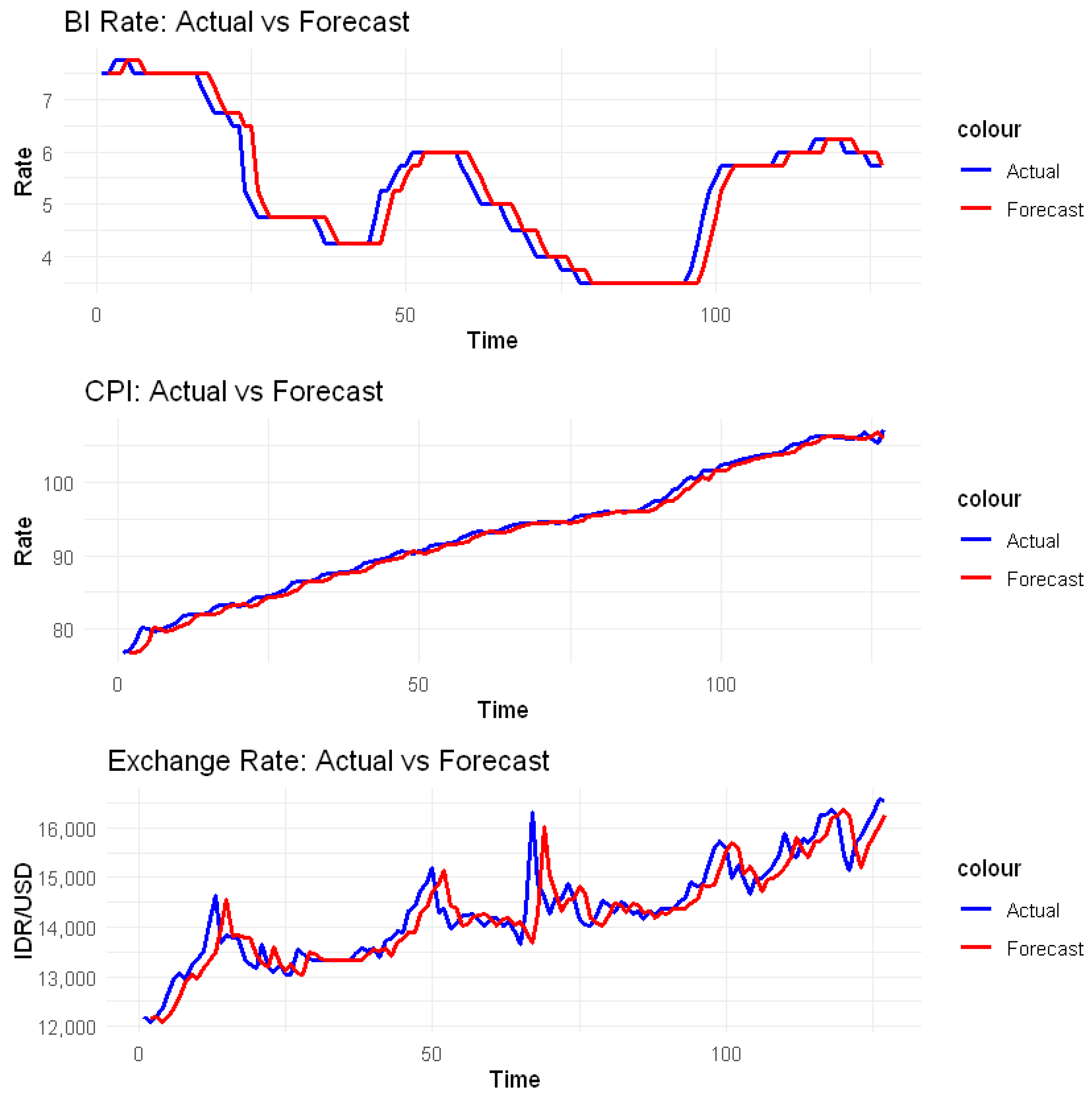
Following Diyah Miasary (2023), the prediction of macroeconomic variables (expected value) is obtained using the simple exponential smoothing (SES) method, the results of which are shown in Figure 2. The red plot in Figure 2 represents the expected value obtained by SES, while the blue plot illustrates the actual value. SES was chosen for prediction because the research data lacked trends and seasonality. Additionally, SES can eliminate noise and adapt to dynamic data changes like financial data. The study by Heo and Kim (2025) utilized SES to improve predictions of financial risk tolerance based on financial market indicators. Smoothing with SES is performed prior to the ARIMA method due to its simplicity, computational speed, and its effectiveness in capturing short-term fluctuations while assigning exponentially decreasing weights to past observations.
Forecast pattern is closed to the actual pattern, demonstrates the accuration and suitability of the SES method for the time series data. The difference between forecast and actual value is calculated as the surprise factor (F). This component is subsequently utilized as an input for sensitivity analysis and impact assessment within the empirical asset return models.
After all variables were computed, a descriptive analysis was conducted to illustrate the patterns and trends in the data (Table 2). All assets exhibited positive R i except for R i B O N D , which recorded a slight negative value of −0.0004. The decline in bond prices is typically offset by higher returns, particularly for short-term bonds (Arshanapalli et al., 2006; Chen et al., 2023). The highest average actual return was observed for R i B T C = 0.0415, followed by R i G O L D = 0.0091 and JKSE at 0.0019. The heightened escalation of global geopolitical risk throughout the study period led investors to favor BTC and gold, both of which experienced sustained price increases, especially during episodes of market turmoil such as the COVID-19 pandemic and extreme macroeconomic shifts (Baur & Lucey, 2010; Paule-Vianez et al., 2020).
Despite their popularity, BTC and gold display markedly different risk profiles. BTC is characterized as a high-risk asset, as evidenced by its large standard deviation (0.2108), while gold is the least risky asset (0.0384) in the sample. JKSE ranks as the second riskiest asset, with a wide range between its minimum (−0.11834) and maximum values (0.0902). The Jarque-Bera statistic for JKSE is notably high, with kurtosis > 3 and skew = 1.0751, indicating a non-normal, leptokurtic distribution with fat tails. Asset evaluation using the EGARCH model and the Student-t distribution is thus particularly appropriate for equities. Both BTC and gold exhibit similar skewness and kurtosis values, with kurtosis close to 3, suggesting near-symmetric distributions. However, their large Jarque-Bera statistics indicate non-normality, making them suitable for GARCH-based modeling. This observation aligns with Baur and McDermott (2010) and Kaczmarek et al. (2022), who assessed gold using GARCH models with a normal distribution.
The use of this model aligns with Ampountolas (2024), who stated that the standard GARCH model provides the best statistical performance when investigating gold volatility during periods of war and financial crises. He tested several models from the GARCH family, including SGARCH, EGARCH, GJR-GARCH, and FI-GARCH, with results showing that the GARCH model was statistically the best, as indicated by the lowest Akaike Information Criterion (AIC) value. This signifies significant volatility clustering and a slightly positive skewness in the return distribution.
In contrast, BTC’s asset evaluation cannot rely on the same approach as gold due to its extremely high Jarque-Bera value and the wide range between its minimum and maximum values, reflecting the presence of extreme data points (Cont, 2001). These characteristics are consistent with the use of the EGARCH model with a Student-t distribution, which provides a more realistic and valid assessment of BTC’s return volatility and risk.
The average inflation surprise was 0.0051, while the exchange rate surprise was 0.0047. These positive values indicate that actual inflation and rupiah depreciation exceeded market expectations. In such an environment, the market anticipates that the central bank will raise interest rates; however, this action would likely reduce the cash flows of firms reliant on debt financing. Over the long term, this would erode corporate earnings and firm value, ultimately leading to a decline in stock prices (Maghrebi et al., 2006).
Throughout the study period, the central bank frequently lowered interest rates to support the domestic investment ecosystem and maintain stock market stability. This is reflected in the negative value of the interest rate surprise, where the predicted value exceeded the actual outcome. This accommodative monetary policy environment provided a buffer for the equity market, mitigating the adverse effects of inflation and currency depreciation on stock performance.
Asset valuation in this study employs the APT-EGARCH model with an order of (1,1). Following Cont (2001), who demonstrated the absence of linear autocorrelation in financial asset returns, the (1,1) specification is adopted for its parsimony and continued relevance for both daily and monthly data frequencies (Nelson, 1991). This order is also consistent in capturing volatility asymmetry and helps to avoid model overfitting (Aftab et al., 2019). The mean equation is estimated using the ARFIMA(1,0,0) approach to detect short-term autoregressive effects and the influence of exogenous variables on actual asset returns. An AR(1) component is included to reduce white noise, thereby ensuring that the error term is stationary and random (Chinzara, 2011). This modeling strategy is supported by empirical literature, which finds that the EGARCH(1,1) model is particularly effective in capturing the leverage effect and volatility clustering in financial time series, while ARFIMA provides flexibility in modeling both short- and long-memory dynamics.
As evident in Table 3, the three surprise factors significantly affect R i J K S E and R i B O N D . The exchange rate shows a negative correlation with both, while the SBI and inflation have a positive effect on stocks but a negative effect on bonds. BOND responds more rapidly to interest rate and inflation news than stocks. In emerging markets, when rising inflation is driven by supply-side increases, central banks tend to hold or even lower interest rates (Maghrebi et al., 2006). Under moderate inflation conditions, such actions increase nominal corporate earnings faster than the rise in the discount rate (Chinzara, 2011). Investors interpret as a positive sentiment that generates buying signals in the capital market.
Empirically, the Indonesian central bank’s policy of maintaining the benchmark interest rate at 4.5% during the spread of COVID-19 until the end of 2020 was effective in restoring the stock market, which had experienced a deep negative contraction. The return of investor confidence was accompanied by various economic stimuli aimed at boosting liquidity and reducing corporate capital costs. This evidence reinforces the view that stock market volatility depends on fundamentals, market structure, and local government policies (Zhu et al., 2025).
Conversely, under high inflation, negative sentiment arises due to economic uncertainty, weakening market prices. The vulnerability of the JKSE to shocks in the exchange rate, SBI, and inflation demonstrates the asymmetric nature of stock markets in developing countries. These findings are consistent with those of Chen et al. (2023), Chinzara (2011), and Maghrebi et al. (2006), but inconsistent with Köse et al. (2024), who concluded that these variables have no significant impact on stock returns.
When the rupiah depreciates, government bonds can serve as a hedge asset within an investor’s portfolio. This result aligns with Arshanapalli et al. (2006) and Mužić and Gržeta (2022), who found that when central banks raise interest rates, bond prices tend to fall—especially for long-term bonds. Newly issued bonds become more attractive due to higher yields. The inverse correlation between equities and bonds with respect to interest rates and inflation highlights the return trade-off between risky and lower-risk assets.
Return and price volatility of an asset will influence the return volatility and prices of other assets (Köse et al., 2024). When bond returns decline due to rising inflation and depreciation of the exchange rate, investors tend to engage in flight-to-safety by moving to the stock market, which offers positive returns (Adrian et al., 2015). Throughout the study period, such conditions occurred several times, including during July–August 2022. Bonds are highly sensitive to macroeconomic news, such as Consumer Price Index (CPI) and Producer Price Index (PPI), which have strong effects in increasing bond market volatility, especially for long-term bonds. Moreover, shocks from interest rate announcements (such as those by the Federal Reserve) show differential responses in short-term and long-term bonds, reflecting differences in time horizons and market risk perceptions.
Additionally, rupiah depreciation prompts investors to seek rupiah-denominated bonds, driving up bond prices in the market. According to bond pricing theory, rising bond prices are accompanied by declining yields. These results are in line with Adrian et al. (2015), Arshanapalli et al. (2006), and Chen et al. (2023), who concluded that bond yields and returns are highly sensitive to macroeconomic changes due to inflation and interest rate expectations.
The AR(1) coefficient is not significant in the equity and bond models, indicating that JKSE and BOND returns are not influenced by their own past values. This finding is consistent with the Random Walk theory, particularly in weak-form efficient markets, where past returns do not predict current returns in the presence of macroeconomic shocks.
The absence of a significant relationship between gold returns and the surprise components of SBI and INF demonstrate strong resilience to both factors. This finding is reinforcing its role as a safe-haven asset, consistent with Arshad et al. (2023), Baur and Lucey (2010) and Terraza et al. (2024). They identify gold as a portfolio hedge during periods of inflation and global interest rate uncertainty. Empirical evidence during the study period, gold repeatedly reached all-time highs, reflecting investors’ flight-to-safety behavior in response to heightened risk in other asset classes. The sensitivity of GOLD returns to exchange rate movements reinforces gold’s role in preserving portfolio value and maintaining investors’ purchasing power, which is eroded by the depreciation of the rupiah (Aftab et al., 2019). The autoregressive component for gold returns is 0.194009 and statistically significant, indicating a momentum effect: when previous returns increase, current returns also tend to rise. This result aligns with Baur and McDermott (2010), who found that gold can exhibit recurring price dynamics during episodes of global uncertainty. The significant autoregressive term also suggests the presence of volatility persistence in gold returns, consistent with Chinzara (2011).
Interestingly, the results show that BTC returns are significantly influenced by all three shock variables as well as by their own lagged values. This finding contradicts Arshad et al. (2023), who argued that BTC is resistant to inflation, government monetary policy (Paule-Vianez et al., 2020), and exchange rate fluctuations (Köse et al., 2024). In this study, inflation exerts a strong and significant negative effect ( β F I N F = 2.642116), indicating that BTC prices are highly responsive to inflation shocks. Empirical evidence from the study period shows a sharp escalation in BTC returns during the global disinflation following the COVID-19 pandemic in 2020. Both interest rates and exchange rates have significant positive effects, supporting Corbet et al. (2020), who found that digital asset returns such as bitcoin can be influenced by interest rate announcements and central bank quantitative easing. The result of C is 0.063667 and significant, indicating that BTC returns are shaped by investor expectations, further supporting the view of bitcoin as a speculative asset. When BTC prices are trending bullish and the rupiah appreciates, aggressive investors tend to increase their BTC holdings. Positive shocks have a greater impact due to heightened investor expectations (Mužić & Gržeta, 2022). These findings reinforce the conclusions of Corbet et al. (2020) and Mužić and Gržeta (2022), who argue that BTC is neither resistant nor resilient to macroeconomic shocks.
Table 4 presents the estimated variance equations for all asset classes. The standard GARCH model applied to gold and the EGARCH(1,1)-X model used for other assets effectively capture volatility clustering, as evidenced by the non-significant ARCH-LM statistics. Under normal conditions, the JKSE exhibits long-term volatility, as indicated by the ω parameter, and persistent volatility, with the β 1 < 0.05. The a 1 + β 1 = 0.684407 suggests that volatility clustering in JKSE dissipates more rapidly compared to BTC. Emerging market stock markets tend to exhibit moderate volatility under normal conditions (Zhu et al., 2025), but volatility becomes extreme during crises such as pandemics, global wars, or domestic geopolitical turmoil (Ampountolas, 2024). Moreover, JKSE is more responsive to negative news than to positive news, as shown by the significant of γ 1 . When the rupiah depreciates, volatility spikes due to market perceptions of economic weakness and foreign capital outflows, whereas rupiah appreciation is not always interpreted as a positive signal (Maghrebi et al., 2006). These findings are consistent with previous studies (Chinzara, 2011; Aftab et al., 2019; Mužić & Gržeta, 2022) that have employed GARCH and EGARCH methodologies.
In contrast, the ω and a 1 for gold and bonds are not significant, indicating that returns on these assets are not sensitive to current or lagged shocks. This study’s findings align with Ampountolas (2024), who confirmed the stability of gold’s volatility clustering using a similar methodology. Gold returns reduce potential losses during shocks (Zhu et al., 2025), but under normal conditions, return growth tends to be slow, especially over the long term (Baur & Lucey, 2010). Both assets display volatility clustering and long-memory dynamics, with persistence values close to 1 and probability values below 0.05, suggesting that long-term memory strongly influences their price movements. The long-term stability of gold further underscores its safe-haven properties during periods of economic uncertainty. This result reinforces earlier research identifying gold as a hedge against exchange rate shocks (Aftab et al., 2019; Bulut & Rizvanoghlu, 2020; Capie et al., 2005), inflation (Arshad et al., 2023), and interest rate volatility. The persistence of bond volatility highlights the bond market’s acute sensitivity to macroeconomic shocks, particularly inflation expectations and monetary policy direction (Arshanapalli et al., 2006). Bond volatility asymmetry, similar to that of JKSE, indicates that negative news induces greater turbulence than positive news.
All parameters of BTC are significant, indicating that BTC volatility surges in response to shocks from previous periods. Additionally, BTC exhibits persistent volatility clustering, with a 1 + β 1 > 1, reflecting non-stationary volatility. The negative asymmetry indicates that positive shocks have a greater impact than negative ones. Positive shocks have a long-lasting, even permanent effect on the volatility of Bitcoin, due to increased return expectations (Mužić & Gržeta, 2022). This response is characteristic of speculative assets, where price movements are dominated by future profit expectations, capital reallocation from other assets, and speculative investor behavior (Corbet et al., 2020; Terraza et al., 2024). Conversely, negative news has a smaller impact, as risk-averse investors tend to hold BTC long-term to avoid short-term losses. This behavior reflects rational investor tendencies, classifying BTC as a speculative-rational asset (Mužić & Gržeta, 2022). These findings are consistent with Köse et al. (2024), who noted that BTC volatility is driven by economic news in the long run and by shocks in the short run.
Goodness-of-fit of model is assessed using AIC, log-likelihood, and the F-LM test for residual heteroskedasticity. Low AIC values across all models indicate strong historical volatility capture, while high log-likelihood values demonstrate good model fit to actual data and the effectiveness of EGARCH in capturing return distribution characteristics. All models passed the ARCH-LM test for heteroskedasticity (Prob.F > 0.05), confirming the absence of residual heteroskedasticity.
Based on the asset evaluation, two portfolios were constructed. The first portfolio is the exercise portfolio, where the weights are assigned based on the expected returns ( E R i ) and the factor loadings of each asset as shown in Table 3. The assumption of portfolio has made by three criteria. First, total assets weight in portfolio equal to 1, formulated by i = 1 n w i = 1 , where w i is the weight of asset. Second, no sensitivity of asset to systematic risk factors, formulated by i = 1 n w i b i = 0 where β ˉ is the weighted average sensitivity of the assets in the portfolio. Last, the expected return of the exercise portfolio ( E R p ) is positive and is mathematically validated as follows. From the asset evaluation results, the following equation is constructed:
0.001972 ω J K S E 0.015253 ω B O N D + 0.010589 ω B T C = 0
0.589940 ω J K S E + 0.322278 ω G O L D 0.408052 ω B O N D + 0.709942 ω B T C = 0
0.806364 ω J K S E 0.706907 ω B O N D 2.642116 ω B T C = 0
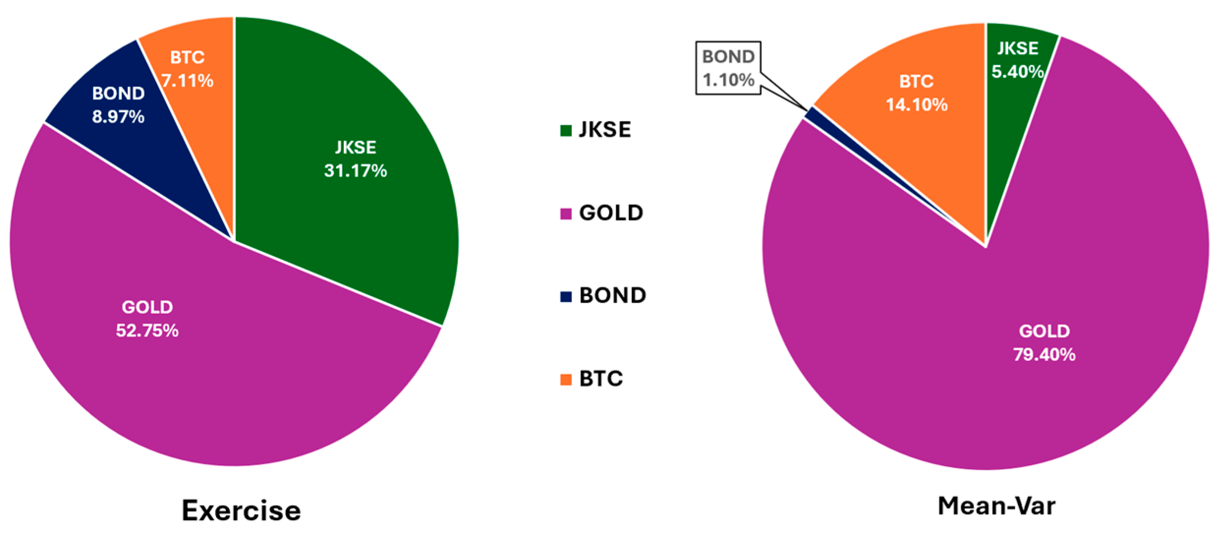
Employing Gauss–Jordan elimination within R Studio (version 4.3.2), the optimal asset allocations were determined to be 52.75% for GOLD, 31.17% for JKSE, 8.97% for BOND, and 7.11% for BTC. To fulfill the third criterion, specifically that the weighted sum of asset returns exceeds unity ( > 1 ), each asset’s proportion was multiplied by its expected return, culminating in a portfolio return of 0.008063 as presented in Table 5. The positivity of this value confirms that the optimization model satisfies the prescribed condition.
The second is a Mean-Var portfolio, in which asset weights are determined using the DE algorithm implemented in R. Allocations optimized the expected portfolio return and minimized risk as measured by VaR at the 95% confidence level. The optimization is performed numerically and stochastically by generating a large number of candidate portfolios (n = 500), subject to the constraint that expected returns must lie above the efficient frontier and risk tolerance is set at the 95% confidence level for all generated portfolios. The selection process is conducted after mutation and recombination steps to identify the optimal candidate. The resulting Mean-Var portfolio consists of 79.4% GOLD, 14.1% BTC, 5.4% JKSE, and 1.1% BOND. The composition of both portfolios is presented in the bar chart in Figure 3 below.
It is unsurprising that gold dominates the portfolio composition. As demonstrated in the single-asset analysis, gold’s persistent resilience to exogenous shocks underscores its role as a safe-haven asset. Positive news asymmetry moderately increases its volatility (Aftab et al., 2019), while negative news often prompts investors to hold gold in anticipation of future price appreciation (Terraza et al., 2024). Gold serves as a wealth-preserving asset, particularly during periods of elevated macroeconomic volatility (Arshad et al., 2023; Capie et al., 2005), deep equity market corrections (Baur & Lucey, 2010), or declines in BTC and bond returns (Arshad et al., 2023; Terraza et al., 2024). The dynamic correlation between gold and bonds further positions gold as a diversification asset for bond portfolios (Paule-Vianez et al., 2020). However, its safe-haven properties may diminish if volatility reaches extreme levels (Baur & McDermott, 2010).
The negative correlation between BOND and the three macroeconomic factors indicates an inverse relationship with increasing shocks (Table 3). While BOND serves as a store of investor wealth, an excessive allocation to BOND in an optimized portfolio—particularly under the constraint of zero sensitivity to systematic risk—may adversely affect portfolio returns. The significant inverse correlation between JKSE and BOND further leads to an overly defensive (over-hedged) portfolio; hence, the optimization method limits the weight of BOND within the portfolio.
The performance of the two optimized portfolios will be compared based on expected returns and portfolio risk. The expected portfolio return is calculated as the weighted sum of each asset’s expected return according to the formula E R p =   i = 1 n w i R i , while the risk is assessed as the weighted sum of asset weights multiplied by their standard deviation ( σ p = i = 1 n w i σ i ). The portfolio exhibiting the highest return with the lowest risk is considered superior in performance. The comparative results are presented in Table 5 below.
Table 5. Comparison of Mean Return and Portfolio Risk.
AssetERStd DevExerciseMean Var
WeightERpStd DevWeightERpStd Dev
JKSE0.0028690.0563000.3117100.0008940.0175490.0540000.0001550.003040
Gold0.0048960.0458400.5275000.0025830.0241810.7940000.0038870.036397
Bond0.0006710.0375600.0897000.0000600.0033690.0110000.0000070.000413
BTC0.0636670.2702100.0711000.0045270.0192120.1410000.0089770.038100
Total 10.0080630.07031010.0130260.077949
Table 5 presents the mean returns of the two portfolios, indicating that the Mean-Variance portfolio exhibits higher expected returns compared to the Exercise portfolio, while their risks are approximately comparable, with Exercise and Mean-Variance risks of 0.070310 and 0.077949, respectively. This outcome suggests superior performance of the Mean-Variance portfolio. Among all individual assets, gold offers the second lowest risk and the second highest mean return. Including gold in the portfolio reduces overall risk and enhances returns during macroeconomic shocks. Aftab et al. (2019) note that flight to quality from risky assets such as equities and Bitcoin to gold reflects its role as a diversifier in emerging markets like Indonesia (Baur & McDermott, 2010).
Bitcoin occupies the second largest allocation due to its highest mean return, which presents an intriguing prospect. Research by Terraza et al. (2024) indicates that Bitcoin’s financialization post-COVID-19 increased its correlation with equities, serving as a short-term diversifier (Paule-Vianez et al., 2020). Bitcoin’s movements show weak and unstable correlation with gold (Mužić & Gržeta, 2022), although under high uncertainty, Bitcoin often moves in tandem with gold (Köse et al., 2024; Paule-Vianez et al., 2020).
Subsequently, portfolio performance was evaluated using a GARCH model incorporating exogenous factors such as inflation shocks, SBI rate, and exchange rate fluctuations, as illustrated in Table 6. The Exercise portfolio exhibits a small but significant negative response to exchange rate shocks and a significant positive correlation with AR(1). Conversely, the Mean-Variance portfolio’s returns are unaffected by macroeconomic shocks, with a non-significant AR(1) term suggesting independence from prior period returns. If exogenous variables remain constant, investors can expect a higher return from the Mean-Variance portfolio (μ = 0.0208511) compared to the Exercise portfolio (m = 0.007848). The variance equation shows persistent leverage effects in the Exercise portfolio with probability of γ 1 is greater than 0.05, necessitating continual asset composition evaluation to safeguard investor wealth from negative shocks. The Mean-Variance portfolio lacks volatility clustering and leverage effects, indicating resilience against extreme negative shocks, making it suitable for conservative to moderate investors.
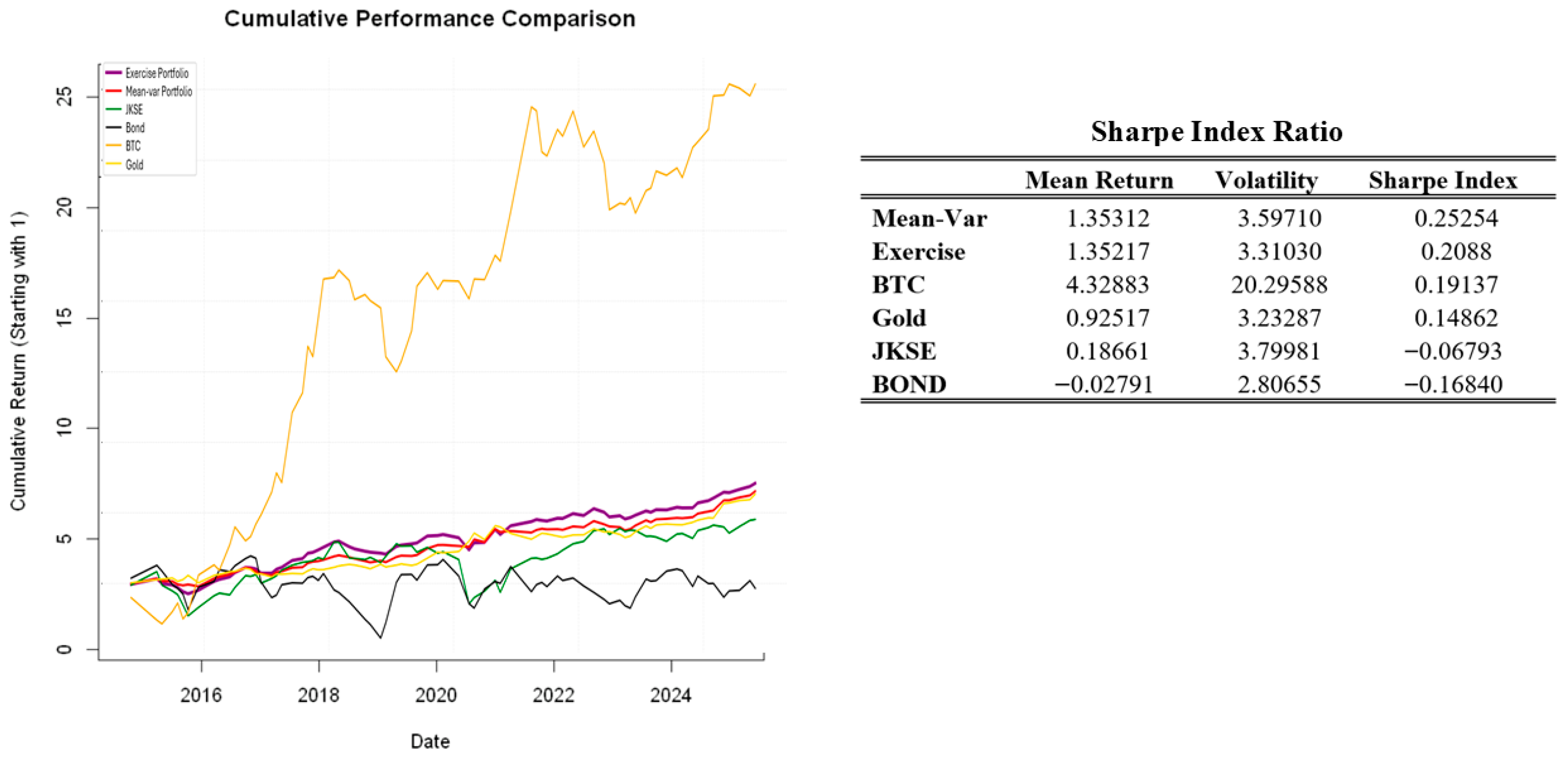
All individual assets and portfolios were evaluated using Cumulative Performance Comparison to assess growth consistency and identify periods of heightened long-term volatility. Portfolio and individual asset performances were further quantified by the Sharpe Ratio Index, measuring the additional return generated per unit of risk, also known as risk-adjusted return. Figure 4 illustrates that the Mean-Variance portfolio achieves stable and consistent growth, whereas the Exercise portfolio, despite showing growth, exhibits more fluctuations.
The Sharpe Ratio for the Mean-Variance portfolio is the highest at 0.25254, outperforming the Exercise portfolio and all individual assets. Furthermore, it delivers higher returns than the Exercise portfolio while exhibiting lower volatility at 3.59710. This confirms that the Mean-Variance portfolio effectively reduces risk without sacrificing returns, aligning with the optimization objective. The diversification achieved mitigates the impact of extreme negative returns on asset volatility and exogenous factor shocks.
Notably, the Sharpe Ratios for JKSE and BOND are unexpectedly negative at −0.06793 and −0.16840, respectively, implying that these assets’ returns do not adequately compensate for their risks. However, BOND exhibits the lowest volatility among all assets and portfolios, underscoring its role as a hedging instrument.
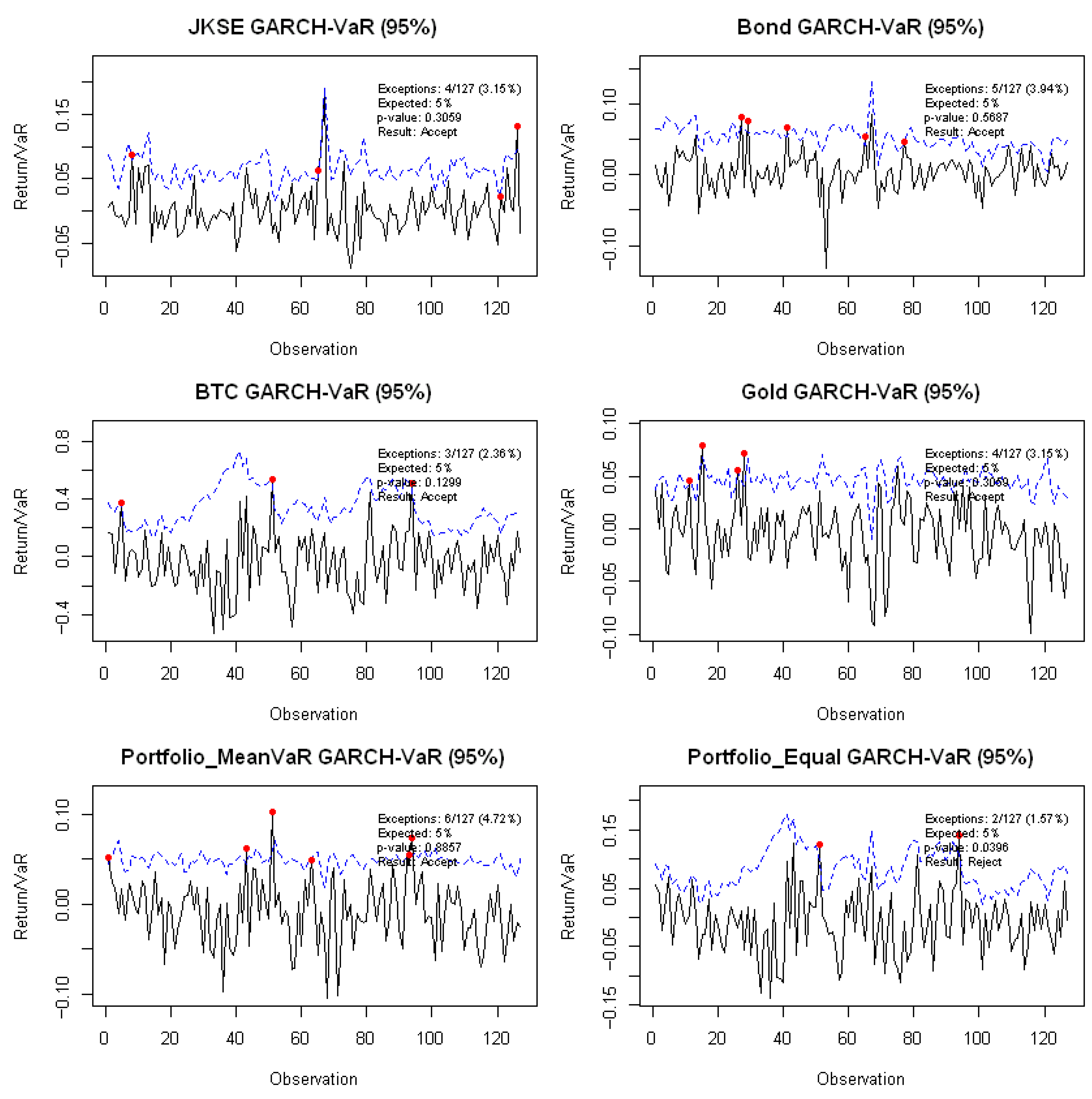
High volatility values observed in the Sharpe Index indicate extreme values driven by exogenous shock factors. Therefore, testing the performance and stability of the developed GARCH model through backtesting is essential (Cont, 2001). This study employs the Kupiec Test to compare actual profit and loss against model predictions (Nieppola, 2009). Violation counts (exceedances) are assessed using the Basel Traffic Light Test, where violations within the Green Zone—ranging from 2 to 6 exceedances out of 127 observations at a 95% confidence level—indicate stable and accurate model performance (Table 7). Exceedances outside this range suggest the model breaches maximum loss thresholds and is vulnerable to shocks.
All individual assets and the Mean-Variance portfolio exhibit exceedances between 3 and 6, placing them within the Green Zone. Both EGARCH and GARCH models effectively capture returns and risks, demonstrating resilience against shocks from SBI rates, exchange rates, and inflation, consistent with historical data. The Kupiec Test results (Figure 5) show a p-value < 0.05, leading to model rejection; however, the Mean-Variance portfolio’s exceedance rate of 4.72% with a p-value of 0.8857 indicates strong empirical and regulatory validity, as this is well above the significance threshold.
In contrast, the Exercise portfolio falls into the Yellow Zone, with more than 6 exceedances, suggesting potential underestimation of tail risk by the EGARCH model due to insufficient capture of the γ parameter. Kupiec’s test for this portfolio yields a violation rate of 5.51%, resulting in model rejection. This supports prior conclusions that the Exercise model is overly optimistic and underestimates extreme risks (tail risk), posing a false sense of security to investors who may incur larger losses during crises.

5. Conclusions and Implications

This study has two primary objectives: first, to assess the return and risk of stocks, gold, BTC, and bonds in response to shocks from changes in inflation, interest rates, and exchange rates; and second, to construct an optimal portfolio comprising these four assets. The sensitivity of asset returns and volatility to shocks in SBI, inflation, and exchange rates varies across asset classes. The findings indicate that gold returns are uncorrelated with inflation and interest rate shocks, but exhibit a positive correlation with exchange rate movements. In Indonesia, gold is highly favored as a safe and highly liquid investment. When the rupiah appreciates, conservative investors in particular tend to hold gold as an alternative investment. Gold’s volatility is moderate, and its cumulative performance demonstrates stable medium- and long-term return growth. The persistence of volatility clustering in gold reflects long-term memory in its price dynamics, affirming Terraza et al. (2024), who found that gold can deliver long-term gains.
Long-term government bond returns display significant negative correlations with all three exogenous variables, consistent with the presence of volatility asymmetry in the variance equation. Negative shocks tend to depress bond prices, especially for long-term bonds. However, shocks such as rising inflation and falling interest rates elicit different responses in short- and long-term bonds, reflecting differences in investment horizon and market risk perception (Arshanapalli et al., 2006; Chinzara, 2011; Mužić & Gržeta, 2022). High volatility persistence indicates long-term effects, but bond returns are not reactive to shocks, highlighting the stability of the bond market, where volatility is trend-driven. When SBI rises, the government typically increases bond coupon rates as an incentive for investors.
The results also show that the Indonesian stock market is highly sensitive to macroeconomic shocks. Consistent with Maghrebi et al. (2006), rupiah depreciation has a more volatile impact than appreciation, indicating volatility asymmetry. Persistent volatility clustering suggests that stock market shocks endure and influence future return volatility. As an emerging market, the JKSE’s volatility asymmetry confirms the significant leverage effect common in such economies, with negative shocks having a greater impact. Throughout the study, the JKSE performed poorly as measured by a negative Sharpe Index. Stock market vulnerability is exacerbated by low domestic investor literacy; when the US dollar and Fed rates rise, foreign investors tend to sell for profit, and domestic investors often follow suit without regard to fundamentals. Impulsive trading decisions can trigger collective panic and increase market risk volatility. Investors are thus advised not to rely solely on equities; when the stock market is under stress, BTC becomes the preferred asset for moderate/aggressive investors.
BTC is highly sensitive to inflation changes but less so to SBI. The EGARCH model captures extreme, persistent volatility clustering and asymmetry, consistent with Cont (2001) on the use of nonlinear volatility models for more realistic asset risk measurement. Positive shocks to BTC have a greater effect due to investor speculation on rising returns, while negative shocks are less likely to prompt selling, as investors hope for long-term gains without fundamental support. This reflects BTC’s speculative-rational nature.
This study has addressed the first objective by confirming that the Jakarta Stock Exchange Composite Index (JKSE), gold (GOLD), government bonds (BOND), and Bitcoin (BTC) respond to shocks in Bank Indonesia’s policy rate (SBI), inflation (INF), and exchange rates with varying sensitivities. Gold exhibits stable volatility and its returns are only sensitive to exchange rate shocks, making it an appropriate portfolio choice during currency depreciation. Conversely, BTC demonstrates extreme volatility in response to all three shock factors, along with persistent volatility asymmetry, reinforcing its nature as a rational speculative asset. Meanwhile, the Indonesian stock and government bond markets show sensitivity to the three macroeconomic factors but in opposite directions. This condition underlines the typical characteristics of emerging market investment environments, which are vulnerable to shocks. When stock market returns decline, investors tend to shift their allocation toward bonds to preserve portfolio value.
Based on the above asset assessment, a Mean-Var portfolio was constructed, consisting of GOLD (79.4%), BTC (14.1%), JKSE (5.4%), and BOND (1.1%). Compared to the Exercise weighted portfolio, the Mean-Var portfolio demonstrates superior performance in terms of Cumulative Performance, with the highest Sharpe Ratio among all assets and the Exercise portfolio, indicating greater efficiency in balancing risk and return. The Mean-Variance portfolio seeks to balance return and risk within its asset composition, aligning with the risk-return tradeoff theory which posits that higher returns serve as compensation for greater risk, particularly in the short term (Köse et al., 2024). In response to exchange rate shocks, domestic investors may increase their gold allocation up to 79.4% of their portfolio to preserve wealth value. Beyond commodity market purchases, the strong tradition in many Asian countries of physically hoarding gold also supports this increased allocation. Conversely, foreign investors tend to refrain from such behavior during similar shocks, instead capitalizing on exchange rate fluctuations for potential gains (Zhu et al., 2025).
Although the average returns of the Mean-Var and Exercise portfolios are almost similar, the Mean-Var portfolio’s returns are not significantly correlated with the three exogenous factors, and macroeconomic shocks do not affect its returns. In the long run, this portfolio is expected to deliver stable and consistent returns, primarily due to the high allocation to gold, which provides better protection. The larger BTC allocation compared to stocks and bonds contributes to higher portfolio returns, but also exposes investors to greater extreme risk, placing the Mean-Var portfolio on the borderline according to the Kupiec Test.
Investors should consider re-evaluating the Mean-Var portfolio during crises, particularly those involving BTC. Reducing BTC exposure during periods of crypto market turbulence is a prudent strategy for preserving asset value. BOND and GOLD are well-suited for conservative investors with medium- to long-term investment horizons, but should be combined with higher-return assets. Purchasing bonds at a discount presents an optimal opportunity for portfolio rebalancing. Additionally, investors may reduce gold allocations in favor of equities during bullish markets, and increasing blue-chip stock holdings can enhance medium-term returns without significantly increasing risk, thereby avoiding opportunity costs.
Domestic investment is likely to increase when economic conditions are stable, as indicated by declining interest rates, exchange rates, and inflation (Amtiran et al., 2017). The exchange rate serves as a channel for economic information that shapes investor risk perceptions (Maghrebi et al., 2006). The managed floating exchange rate system adopted by the government provides the central bank with flexibility to set adaptive interest rates and control inflation. Policymakers should implement an inflation-targeting framework as a shock absorber for abnormal stock market volatility.
Monetary policy decisions by the Indonesian government influence market volatility. During the study period, the central bank adjusted interest rates several times to maintain economic stability, such as in October 2023, when heightened global geopolitical risk and US monetary tightening prompted an unexpected rate hike, strengthening the exchange rate and preventing imported inflation. Currently, accommodative monetary and expansionary fiscal policies have helped maintain Indonesia’s economic fundamentals during economic shocks.
The main contribution of this study is the construction of an optimal portfolio from four distinct asset classes utilizing the Differential Evolution optimization algorithm accompanied by the Mean-Variance approach. Gold dominates asset allocation as a wealth preservation instrument during crises, while Bitcoin exhibits persistent positive asymmetry and significantly diversifies portfolio returns. Backtesting procedures employing the Kupiec test and Basel Traffic Light method validate that risk estimation via GARCH models meets international regulatory standards, enabling portfolios with superior risk-adjusted performance compared to equal-weight alternatives. This study offers an empirical contribution of considerable relevance to investment management and monetary policy formulation in emerging markets.
Additionally, it affirms the efficacy of applying the EGARCH(1,1) model to capture volatility dynamics in both individual assets and portfolios, notably volatility clustering and asymmetry, as described by Cont (2001). Overall, the model effectively visualizes asset characteristics based on realized return and risk. Model evaluation using the Sharpe Ratio and Cumulative Performance confirms that the Mean-Var portfolio is optimal for investors and investment managers in Indonesia. However, the gold-dominated Mean-Var composition may be less attractive to aggressive investors seeking higher returns. Investors with higher risk tolerance may consider greater BTC exposure, using VaR-based risk mitigation, while retaining GOLD and BOND as stabilizers against BTC’s extreme volatility.

6. Future Research

This study is limited to evaluating four asset classes in response to shocks from three exogenous factors in Indonesia, with the results used to construct an optimal portfolio applicable to Indonesian investors. There remains considerable scope for future research, such as incorporating additional macroeconomic shocks or including alternative asset classes like CPO, ESG-based instruments, or digital assets beyond Bitcoin to test the robustness of broader portfolio diversification.
Further exploration of the hedging and safe-haven functions of these four instruments during crisis conditions also presents a promising avenue for future work. Expanding comparative studies between emerging and developed markets in Asia would provide valuable perspectives for both investors and regulators. Given the global environment’s heightened vulnerability to various issues, the likelihood of extreme crises is increasing. Advanced econometric approaches, such as stochastic volatility models or copula-GARCH, could be employed to capture nonlinear dependencies and tail risk. Finally, integrating behavioral finance perspectives that account for investor heterogeneity and asset selection in portfolio construction would be highly relevant, offering practical portfolio recommendations for both individual investors and risk managers.

Author Contributions

Conceptualization, V.M.N.; Methodology, V.M.N.; Software, V.M.N.; Validation, V.M.N., H.S., R.S. and N.Z.; Formal analysis, V.M.N.; Investigation, V.M.N.; Resources, V.M.N.; Data curation, V.M.N.; Writing—original draft, V.M.N.; Writing—review & editing, V.M.N., H.S., R.S. and N.Z.; Visualization, V.M.N.; Supervision, H.S., R.S. and N.Z. All authors have read and agreed to the published version of the manuscript.

Funding

This research was funded by the Indonesian Endowment Fund for Education (LPDP). The authors appreciate their full commitment and generous funding, which was instrumental in the completion of my doctoral education. The sustained support from LPDP directly facilitates my professional goal of enhancing academic proficiency to improve the quality of instruction for my students.

Institutional Review Board Statement

Not applicable.

Informed Consent Statement

Not applicable.

Data Availability Statement

The data were derived from the following resources available in the public domain: http://www.investing.com (accessed on 17 April 2023), https://www.coindesk.com/price/BTC/ (accessed on 17 April 2023), https://www.bps.go.id (accessed on 17 April 2023), https://www.bi.go.id (accessed on 17 April 2023).

Conflicts of Interest

The authors declare no conflict of interest.

References

  1. Adrian, T., Crump, R. K., & Vogt, E. (2015). Nonlinearity and flight to safety in the risk-return trade-off for stocks and bonds. The Journal of The American Finance Association, 74(4), 2019. [Google Scholar]
  2. Aftab, M., Shah, S. Z. A., & Ismail, I. (2019). Does gold act as a hedge or a safe haven against equity and currency in Asia? Global Business Review, 20(1), 105–118. [Google Scholar] [CrossRef]
  3. Ampountolas, A. (2024). Enhancing forecasting accuracy in commodity and financial markets: Insights from GARCH and SVR models. International Journal of Financial Studies, 12(3), 59. [Google Scholar] [CrossRef]
  4. Amtiran, P. Y., Indiastuti, R., Nidar, S. R., & Masyita, D. (2017). Macroeconomic factors and stock returns in APT framework. International Journal of Economics and Management, 11(S1), 197–206. [Google Scholar]
  5. Arshad, S., Vu, T. H. N., Warn, T. S., & Ying, L. M. (2023). The hedging ability of gold, silver and bitcoin against inflation in asean countries. Asian Academy of Management Journal of Accounting and Finance, 19(1), 121–153. [Google Scholar] [CrossRef]
  6. Arshanapalli, B., d’Ouville, E., Fabozzi, F., & Switzer, L. (2006). Macroeconomic news effects on conditional volatilities in the bond and stock markets. Applied Financial Economics, 16(5), 377–384. [Google Scholar] [CrossRef]
  7. Baur, D. G., & Lucey, B. M. (2010). Is gold a hedge or a safe haven? An analysis of stocks, bonds and gold. Financial Review, 45(2), 217–229. [Google Scholar] [CrossRef]
  8. Baur, D. G., & McDermott, T. K. (2010). Is gold a safe haven? International evidence. Journal of Banking and Finance, 34(8), 1886–1898. [Google Scholar] [CrossRef]
  9. Beckmann, J., Berger, T., & Czudaj, R. (2015). Does gold act as a hedge or a safe haven for stocks? Rurh economic paper No. 502. Available online: https://papers.ssrn.com/sol3/papers.cfm?abstract_id=2561224 (accessed on 2 February 2024).
  10. Bulut, L., & Rizvanoghlu, I. (2020). Is gold a safe haven? The international evidence revisited. Acta Oeconomica, 70(4), 531–549. [Google Scholar] [CrossRef]
  11. Campbell, J. Y., Lo, A. W., & MacKinlay, A. C. (1997). The econometrics of financial markets. Macroeconomic Dynamics, 2(4), 559–562. [Google Scholar] [CrossRef]
  12. Capie, F., Mills, T. C., & Wood, G. (2005). Gold as a hedge against the dollar. Journal of International Financial Markets, Institutions and Money, 15(4), 343–352. [Google Scholar] [CrossRef]
  13. Chen, Y. F., Chiang, T. C., & Lin, F. L. (2023). Inflation, equity market volatility, and bond prices: Evidence from G7 countries. Risks, 11(11), 191. [Google Scholar] [CrossRef]
  14. Chinzara, Z. (2011). Macroeconomic uncertainty and conditional stock market volatility in South Africa. South African Journal of Economics, 79(1), 27–49. [Google Scholar] [CrossRef]
  15. Cont, R. (2001). Empirical properties of asset returns: Stylized facts and statistical issues. Quantitative Finance, 1(2), 223–236. [Google Scholar] [CrossRef]
  16. Corbet, S., Larkin, C., Lucey, B. M., Meegan, A., & Yarovaya, L. (2020). The impact of macroeconomic news on Bitcoin returns. European Journal of Finance, 26(14), 1396–1416. [Google Scholar] [CrossRef]
  17. Diyah Miasary, S. (2023). Penentuan Return Saham Syariah dengan Arbitrage Pricing Theory (APT) melalui Pendekatan Vector Autoregressive (VAR). Jurnal Axioma: Jurnal Matematika dan Pembelajaran, 8(2), 124–134. [Google Scholar] [CrossRef]
  18. Global Crypto Adoption Index. (2024). The 2024 global adoption index: Central & Southern Asia and Oceania (CSAO) region leads the world in terms of global cryptocurrency adoption. Available online: https://www.chainalysis.com/blog/2024-global-crypto-adoption-index/ (accessed on 2 February 2024).
  19. Heo, W., & Kim, E. (2025). Smoothing the subjective financial risk tolerance: Volatility and market implications. Mathematics, 13(4), 680. [Google Scholar] [CrossRef]
  20. Kaczmarek, T., Będowska-Sójka, B., Grobelny, P., & Perez, K. (2022). False safe haven assets: Evidence from the target volatility strategy based on recurrent neural network. Research in International Business and Finance, 60(c), 101610. [Google Scholar] [CrossRef]
  21. Köse, N., Yildirim, H., Ünal, E., & Lin, B. (2024). The Bitcoin price and Bitcoin price uncertainty: Evidence of Bitcoin price volatility. Journal of Futures Markets, 44(4), 673–695. [Google Scholar] [CrossRef]
  22. Maghrebi, N., Holmes, M. J., & Pentecost, E. J. (2006). Are there asymmetries in the relationship between exchange rate fluctuations and stock market volatility in pacific basin countries? Review of Pacific Basin Financial Markets and Policies, 9(2), 229–256. [Google Scholar] [CrossRef]
  23. Markowitz, H. (1952). Portofolio selection. The Journal of Finance, 7(1), 77–91. [Google Scholar]
  24. Mužić, I., & Gržeta, I. (2022). Expectations of macroeconomic news announcements: Bitcoin vs. traditional assets. Risks, 10(6), 123. [Google Scholar] [CrossRef]
  25. Nelson, D. B. (1991). Conditional heteroskedasticity in asset returns: A new approach. Econometrica, 59(2), 347–370. [Google Scholar] [CrossRef]
  26. Nieppola, O. (2009). Backtesting value-at-risk models. Journal of Financial Econometrics, 9(2), 314–343. [Google Scholar]
  27. Nurbarani, B. S., & Soepriyanto, G. (2022). Determinants of investment decision in cryptocurrency: Evidence from Indonesian investors. Universal Journal of Accounting and Finance, 10(1), 254–266. [Google Scholar] [CrossRef]
  28. Paule-Vianez, J., Prado-Román, C., & Gómez-Martínez, R. (2020). Economic policy uncertainty and Bitcoin. Is Bitcoin a safe-haven asset? European Journal of Management and Business Economics, 29(3), 347–363. [Google Scholar] [CrossRef]
  29. Roll, R., & Ross, S. A. (1995). The arbitrage pricing theory approach to strategic portfolio planning. Financial Analysts Journal, 51(1), 122–131. [Google Scholar] [CrossRef]
  30. Selmi, R., Mensi, W., Hammoudeh, S., & Bouoiyour, J. (2018). Is Bitcoin a hedge, a safe haven or a diversifier for oil price movements? A comparison with gold. Energy Economics, 74, 787–801. [Google Scholar] [CrossRef]
  31. Terraza, V., Boru İpek, A., & Rounaghi, M. M. (2024). The nexus between the volatility of bitcoin, gold, and american stock markets during the COVID-19 pandemic: Evidence from VAR-DCC-EGARCH and ANN models. Financial Innovation, 10(1), 22. [Google Scholar] [CrossRef]
  32. Zhu, Y., Taasim, S. I., & Daud, A. (2025). Volatility modeling and tail risk estimation of financial assets: Evidence from gold, oil, bitcoin, and stocks for selected markets. Risks, 13(7), 138. [Google Scholar] [CrossRef]
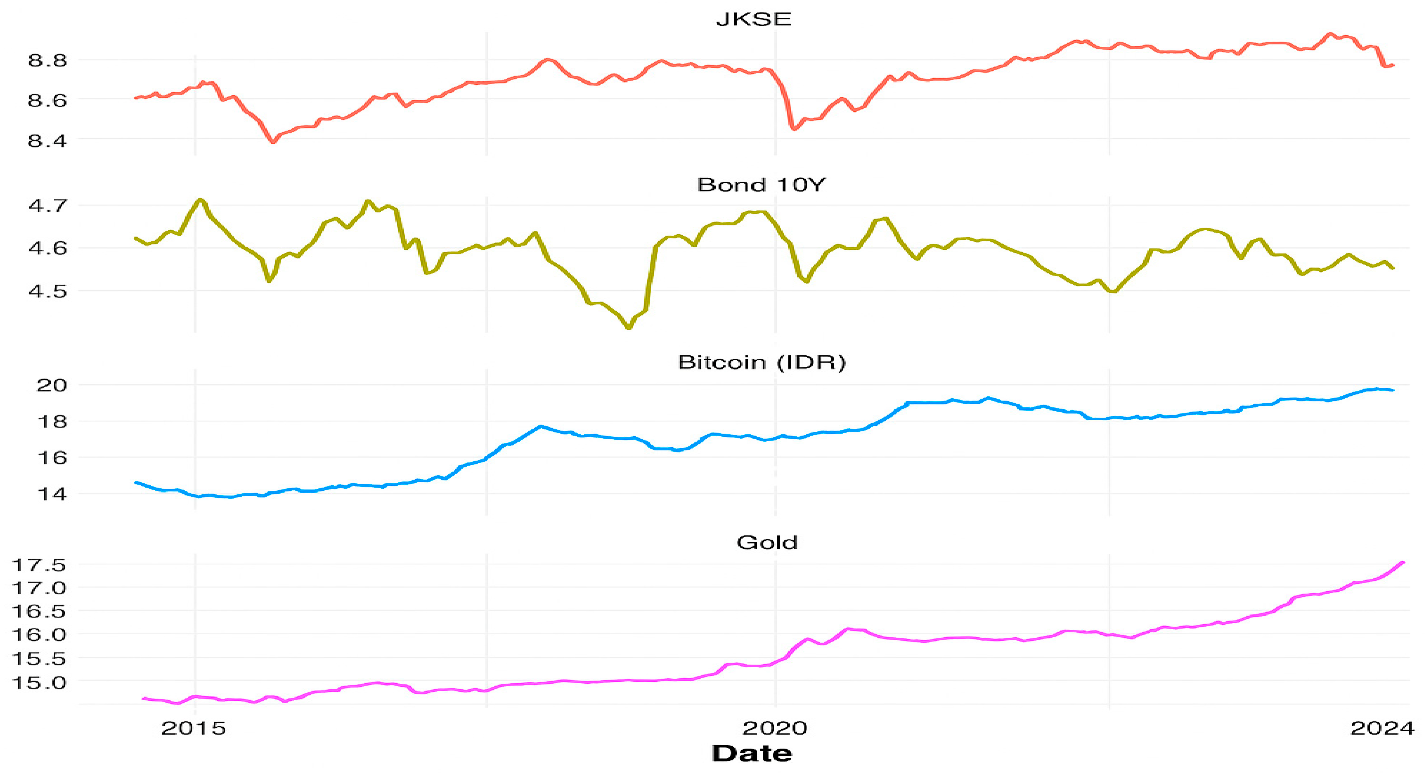
Figure 1. Monthly Log Closing Price of Assets.
Jrfm 18 00668 g001
Figure 2. Forecast of Exc, Inf and SBI.
Jrfm 18 00668 g002
Figure 3. Composition of Assets in Portfolio. Source: Processed by Author.
Jrfm 18 00668 g003
Figure 4. Cumulative Perfomance Comparison and Sharpe Index Ratio.
Jrfm 18 00668 g004
Figure 5. Kupiec Test of Assets and Portfolios.
Jrfm 18 00668 g005
Table 1. Literature Review.
AuthorAssetEconomic MacroMethodResult
Arshanapalli et al. (2006) and Chen et al. (2023)Bond and stockInterest rate, inflation, PPIGARCHThe GARCH model is capable of capturing asymmetric effects in stock and bond markets, which are characterized by heteroskedasticity and volatility clustering.
Mužić and Gržeta (2022)Gold, bond and BTCInflation, NFP, Initial Jobless Claims, Retail Sales and IPIGARCH and EGARCHBonds are highly sensitive to shocks, in contrast to Bitcoin (BTC), which exhibits more varied responses to market disturbances. Gold, on the other hand, demonstrates greater stability and consistently displays the attributes of a safe-haven asset.
Köse et al. (2024)BTCEPU, goldprice and exchange rateGARCHBTC responds to shocks with heterogeneous reactions, reflected in its pronounced volatility.
Terraza et al. (2024)BTC, gold and stockCorona Virus spreadVAR-DCC-EGARCHBTC exhibits significant volatility persistence compared to equities, whereas gold maintains relative stability with more moderate and consistent levels of volatility.
Arshad et al. (2023)Gold, silver, BTCCPIStudent-t EGARCH(1,1) and Quantile RegressionAll three assets function as hedges and safe-haven assets, with their roles contingent upon prevailing return levels and inflation conditions.
Chinzara (2011)StocksIPI, CPI, money supply, exchange rate, oil price, T-Bills and gold priceAR-GARCH, EGARCH, TARCH and VARTreasury Bill and exchange rate volatility are identified as the most significant drivers of stock market volatility.
Chen et al. (2023)Stocks and BondsCPIVAR, FAVAR and GARCHInflation shocks substantially increase equity volatility, while bond prices tend to decline in response to similar events, reflecting rising yield expectations.
Aftab et al. (2019)Stocks and goldExchange rateDCC-MGARCHAsian equities exhibit moderate volatility, yet their respective stock markets are characterized by high overall volatility.
Ampountolas (2024)Gold, stocks, commoditiesFinancial marketevent studiesSGARCH, EGARCH, GJR-GARCH, and FI-GARCHGold displays persistent and long-term volatility clustering, as indicated by SGARCH modeling.
Zhu et al. (2025)Stocks, BTC, oil and gold priceVolatility of assetsEGARCH, AR, Extreme Value Theory (EVT), rolling window estimation, and distribusi skewed heavy-tail.Among the assets analyzed, gold consistently demonstrates the lowest volatility, in stark contrast to bitcoin, which is significantly more volatile. Equities in emerging markets have medium volatility levels, but these can escalate sharply in the wake of macroeconomic shocks.
Table 2. Descriptive Analysis.
R i F
JKSEGOLDBONDBTCSBIEXCINF
Mean0.00190.0091−0.00040.0415−0.02780.00470.0051
Median0.00590.006−0.00210.05040.00000.00540.0043
Max0.09020.10410.13720.53161.00000.16060.0385
Min−0.1834−0.0728−0.0829−0.5328−1.5000−0.0967−0.0125
Std.Dev0.03930.03840.04250.21080.02900.00270.0005
Skew−1.07510.34150.39030.3541−0.26860.44071.4608
Kurtosis6.76812.4184.12592.74925.36594.95826.7882
JB392.23167.75391.04117.591226.26960.714767.96
Source: Processed by Author. Note: R i denotes the actual return of stock at time t; R i g refers to the return of gold; R i b represents the return of the bonds; R i b t c is the actual return of bitcoin at time t. FSBI is the loading factor of interest rate of Indonesia central banks; FEXC refers to the loading factor of exchange rate and FINF denotes the inflation’s loading factor.
Table 3. Mean Equation.
R i CAR(1) β F S B I β F E X C β F I N F
J K S E 0.002869 *−0.1253160.001972 *−0.589940 *0.806364 *
G O L D 0.0048960.194009 *−0.006310.322278 *−0.36786
B O N D 0.000671−0.054078−0.015253 *−0.408052 *−0.706907 *
B T C 0.063667 *0.034123 *0.010589 *0.709942 *−2.642116 *
Source: Processed by Author. Note: In the mean regression analysis, variable C represents the instrument expected return while AR(1) is included to reduce white noise, thereby ensuring that the error term is stationary and random. The β F S B I , β F E X C and β F I N F represent the coefficien of surprise factors of exchange rate, inflation, and interest rate on the instrument, respectively. * denotes significance at 5%, respectively.
Table 4. Variance Equation.
AssetVariance EquationAICLLF-LM
ω a 1 β 1 a 1 + β 1 γ 1
J K S E −2.078196 *−0.0139220.698329 *0.6844070.391663 *−3.9713261.17690.8791
G O L D 0.0000000.0000000.999000 *0.999000-−4.0201265.27420.2750
B O N D 0.000388−0.0146240.994674 *0.9891610.107711 *−4.5090295.32170.4409
B T C −0.101840 *0.227942 *0.968559 **1.104781−0.293953 *−0.4800739.484550.8961
Source: Processed by Author. Note: ω represents the intercept of the variance equation and corresponds to a free shock component, while a 1 denotes the sensitivity to past shocks. The coefficient β 1 reflects the persistence of volatility clustering, and the sum of a 1 + β 1 illustrates the overall dynamics of volatility within the specified model. The parameter γ 1 captures the asymmetric volatility effect measured in the EGARCH model. F-LM refers to the ARCH test for heteroscedasticity; LL indicates the log-likelihood ratio; and AIC denotes the Akaike Information Criterion. * and ** represent statistical significance at the 5% and 10% levels, respectively.
Table 6. Mean And Variance Equation of Portfolio.
Equation Exercise PortfolioMean-Var Portfolio
MeanC0.007848 *0.010851
AR(1)0.192558 **0.081365
β F S B I 0.0019820.081365
β F E x c −0.000070 *0.156908
β F I n f −0.004875−0.566213
Variance ω −0.3258470.000001
a 1 −0.1569420.000000
β 1 0.566165 *0.999000 *
a 1 + β 1 0.4092230.999000
γ 1 0.914650 *-
Source: Processed by Author. Note: * denotes significance at 5% and ** is significance at 10%, respectively.
Table 7. Basel Traffic Test.
Portfolio/AssetConfidence LevelNumber of
Observation
Number of ExceptionsTest Outcome
JKSE95%1274Green Zone
Bond95%1275Green Zone
BTC95%1273Green Zone
Gold95%1274Green Zone
Mean-VaR Portfolio95%1276Green Zone
Exercise Portfolio95%1277Yellow Zone
Source: Processed by Author.
Disclaimer/Publisher’s Note: The statements, opinions and data contained in all publications are solely those of the individual author(s) and contributor(s) and not of MDPI and/or the editor(s). MDPI and/or the editor(s) disclaim responsibility for any injury to people or property resulting from any ideas, methods, instructions or products referred to in the content.