Split-Screen Approach to Financial Modeling in Sustainable Fleet Management

Abstract

Large-scale transitions to eco-friendly vehicle fleets present complex capital budgeting challenges, requiring the integration of extensive operational data with financial modeling while balancing economic profitability and environmental sustainability. Traditional approaches often struggle to manage this complexity and quantify the inherent trade-offs. This study develops and applies an innovative integrated accounting-and-finance framework to evaluate the economic and environmental implications of green fleet transition projects, explicitly quantifying the trade-off between profitability and sustainability. Focusing on waste vehicle replacement of Iren Spa, a leading European multi-utility company, we employ the recently developed Split-Screen Approach, a unified accounting-and-finance framework grounded in the laws of motion and conservation. It automatically reconciles pro forma financial statements and generates internally consistent valuation metrics, eliminating the manual adjustments and inconsistencies of traditional models. Its built-in diagnostic checks and scalability for highly complex datasets overcome the manual adjustments and inconsistencies inherent in traditional financial models. We process 2303 inputs across multiple “green” scenarios. This methodology integrates an Engineering Model, describing fleet evolution, operating costs, and CO₂ reduction, with a HookUp Model, which serves to transform scenarios into well-defined projects. The latter model is then integrated with a Financial Model that generates pro forma financial statements, incorporates financing and payout policies, and assesses economic profitability through Net Present Value (NPV) and consistent accounting rates of return. Together, these elements form a robust framework for managing complex data integration and analysis. Our research reveals a fundamental trade-off: enhanced environmental sustainability (measured by Net Green Value, NGV), which quantifies CO₂ reduction, is achieved at the expense of economic profitability, measured by NPV. This financial sacrifice is captured by the Net Value Curve, a Pareto frontier, while the NPV-to-NGV ratio provides “shadow prices” for CO₂ reduction, revealing the financial cost per unit of sustainability gained. Based on 21 project scenarios and additional sensitivity analyses on financial inputs and energy prices, the results confirm a decreasing relationship between NGV and NPV. This study makes three main contributions: (1) it demonstrates the practical application of the Split- Screen Approach for capital budgeting under complexity, (2) it introduces the Net Value Curve framework as a useful tool for visualizing and quantifying the trade-off between profitability and sustainability, (3) it provides managers and policymakers actionable insights, supporting more informed decisions in green fleet transition planning where economic and environmental objectives may conflict. The findings provide managers and policymakers with a rigorous and transparent accounting-and-finance framework that enhances the reliability of capital budgeting decisions compared with traditional financial modeling, while offering a Paretian frontier for evaluating environmental trade-offs.

1. Introduction

Vehicle replacement policies play a central role in the waste management industry due to their direct impact on operational efficiency, environmental sustainability, and financial performance. Fleet vehicles are essential for waste collection, transportation, and disposal, and their aging or inefficiency can lead to increased maintenance costs, higher emissions, and reduced service reliability. Transitioning to eco-friendly fleets, such as electric or hybrid vehicles, is increasingly prioritized to meet stringent environmental regulations and corporate sustainability goals. However, balancing the economic viability of such transitions with environmental benefits remains a significant challenge. This study investigates the intersection of sustainability and profitability within vehicle replacement decisions. We introduce a new integrated accounting-and-finance system designed to assist business decision-makers concerned with both shareholder value creation and environmental sustainability. Specifically, our focus centers on the challenge faced by an Italian company, Iren Ambiente, a subsidiary of Iren Spa, a leading Italian multi-utility company, to explore this trade-off in a real-world context and define a strategic plan in alignment with IREN Group’s Action plan for “green” mobility. Italy’s waste management sector, with its unique regulatory and infrastructural constraints, provides an ideal setting to examine the complexities of sustainable fleet transitions. Our analysis studies the bi-objective problem (sustainability vs. profitability) of vehicle replacement policies within the waste management industry, exploring various plans for Iren Ambiente’s fleet of 1435 vehicles under different fuel selection policies. This paper aims to quantify in a rigorous way the economic value associated with a given replacement policy and, in addition, to measure the CO₂ emission reduction associated with each green scenario. This study offers actionable insights for similar organizations addressing the objective of analyzing economic profitability and take into account the degree of sustainability for each scenario considered.

While replacement projects fall within the realm of capital budgeting projects, which is a primary focus in corporate finance, they are often approached differently in the engineering literature (further discussed in the following section). Engineering emphasizes a project’s operational facets: it explores the technical intricacies, optimization processes, and the selection of suitable tools to maximize (or minimize) some objective function within a set of constraints. In contrast, finance centers on assessing the economic value generated by the project: pro forma financial statements are constructed to estimate book values of assets, revenues, costs, earnings, and cash flows associated with the project. These calculations aid in determining the project’s economic profitability, typically using some financial metric such as the Net Present Value or some rate of return. This assessment assists companies in making economically sound evaluations of projects. A financial analyst often overlooks operational subtleties and opts for a narrower set of parameters to streamline the financial model. Conversely, engineers may tend to simplify or disregard accounting elements and eliminate financial complexities in an effort to streamline the operational model. Both perspectives emphasize one aspect while overlooking the essential connection between engineering and finance. Recognizing the potential for mutual benefit, this paper highlights that both fields can complement each other and aims to merge the two perspectives using a new integrated accounting-and-finance model, developed in Magni (2020, 2023). This framework refines traditional financial modeling by systematically integrating engineering and accounting dimensions, incorporating the firm’s payout and retention policy, and applying diagnostic tools that validate the financial model, thus helping to avoid common errors found in conventional modeling (see Baschieri & Magni, 2023; Magni, 2025).

A core contribution of this study is the application of the Split-Screen Approach (SSA), a novel accounting-and-finance system that introduces unprecedented rigor in modeling capital budgeting projects (see Magni, 2020, 2023; Baschieri & Magni, 2023; Magni, 2025).

Existing literature relies heavily on optimization techniques using simplified financial models and proxies (see section on literature review below), which fail to capture the intricate interdependencies between operational drivers, accounting constructs, and financial valuation. This gap is especially critical for complex projects, where thousands of inputs dynamically interact (e.g., asset lifespans, tax policies, debt schedules) across a multi-year horizon. How can a capital budgeting framework integrate a vast set of operational and financial inputs into a dynamically consistent model that preserves accounting-valuation coherence, explicitly incorporates payout and financing policies, and automatically reconciles pro forma financial statements with project valuation metrics, thereby overcoming the limitations of traditional modeling techniques? The SSA addresses this by establishing dynamic linkages within financial statements and between financial statements and value creation, using the Split-Screen Matrix (SSM) framework and built-in diagnostic tools (see Magni, 2020, 2023, 2025). Unlike previous contributions, this paper

• integrates engineering outputs with pro forma financial statements (balance sheets, income statements, cash flow statements);
• measures financial efficiency across operating, non-operating, debt, and equity areas using consistent metrics such as NPV, residual income, average accounting rates of return;
• processes 2303 inputs dynamically—including vehicle-specific costs, tax effects, working-capital policy, and debt schedules—into 105 interdependent financial statements through automated accounting linkages, offering a level of granularity unattainable with existing capital budgeting tools.

This automation ensures dynamic accounting consistency over time, eliminating the manual reconciliations typical of standard models. To our knowledge, no prior study has offered a financial valuation of comparable analytical complexity for a capital budgeting project of this scale.

This work represents the first implementation of the SSA for a capital budgeting project of this scale and complexity (2303 inputs, 1435 vehicles, 50 vehicle types, 17-year horizon). By applying it to Iren Ambiente’s fleet, a context with high vehicle heterogeneity and strict operational constraints, we demonstrate how the SSA enables scalable, robust financial modeling for any large-scale capital budgeting project, regardless of complexity or volume.

We start from what we call the “Engineering model”, incorporating a very large number of operational inputs, which feed into a robust accounting-and-financial model, capable of assessing the economic profitability across multiple scenarios. More specifically, we manage a total of 2303 inputs across five “green scenarios”, enabling simultaneous analysis and comparison, matching economic profitability with environmental sustainability. The primary output is represented by the “Net Value” curve, which illustrates the combination of Net Present Value (NPV) for the value creation and the Net Green Value (NGV) for CO₂ emission reduction. As the NGV increases, both project NPV and equity NPV decrease, testifying of a decreasing relation between economic value and environmental value. In other words, we find a trade-off between “being greener” and “being richer”. The Net Value curve is then a Pareto frontier quantifying how much value the company must give up to increase the degree of its environmental sustainability. The ratio of the NPV to the NGV supplies the “shadow” prices of a one-ton CO₂ reduction, providing precise quantification of IREN’s sacrificed value for every ton of CO₂ reduction in each green scenario. The shadow prices are increasing with respect to the degree of sustainability of a replacement policy: the more environmentally friendly the replacement policy adopted, the greater the financial sacrifice. To further investigate the functional relation between the NGV and the NPV, we expand the analysis to additional 16 green scenarios, up to a total of 21 scenarios. This extended scope offers a comprehensive view of the NPV sacrifice concerning CO₂ total reduction ranging from 0 to 140,000 tons. The outcome reveals a strictly decreasing, concave function of NGV, with an increasing marginal rate of substitution, as verified by a degree-2 polynomial regression with a remarkably high coefficient of determination (R² = 0.9935).

The architecture of our accounting-and-finance system is developed within a spreadsheet software, which is publicly available at https://doi.org/10.5281/zenodo.17381603. It includes a first section that collects the inputs, classified into five classes:

(i)

operating inputs (influencing the value of operating assets and liabilities),

(ii)

non-operating inputs (impacting the balance of liquid assets),

(iii)

debt inputs (affecting the company’s outstanding debt),

(iv)

equity inputs (influencing the equity capital),

(v)

market data (affecting the required rates of return).

The technical inputs are processed within the Engineering model with the purpose of calculating the total CO₂ reduction associated with each scenario (NGV) and of feeding the HookUp model, which is designed to bridge the engineering and financial perspectives. This model also processes debt data and other operational inputs, converting the five scenarios into five distinct projects. The outputs of the HookUp model, along with the remaining inputs, are then fed into the Financial model, which finalizes the financial planning and performs the financial valuation and efficiency analysis. For the construction of pro forma financial statements, we adopt the SSA and manage intrinsic operational risk using the well-known Capital Asset Pricing Model (CAPM). The market value of operating assets is assessed using the Adjusted Present Value (APV) method (Myers, 1974), enabling the computation of NPVs. Rates of return and financial efficiencies for each project are also calculated. Ultimately, the NPV and the NGV together form the Net Value curve. The remainder of the paper is structured as follows. Section 2 offers the background framework encompassing vehicle replacement problems, financial planning, and project appraisal methods. Section 3 provides insights into green mobility within IREN’s Action Plan. Section 4 introduces the problem, outlines its architecture, and details the spreadsheet composition used for the development of the engineering-and-finance system. Section 5 illustrates the inputs. Section 6 describes the Engineering model. Section 7 explains the HookUp model. Section 8 presents the Financial model. Section 9 shows and discusses the outputs. Section 10 contains concluding remarks.1

2. Literature Review

In capital budgeting analysis, replacement projects are one of three types: expansion projects, abandonment projects, and replacement projects. Modeling the latter is more difficult because they exhibit characteristics of both expansion projects and abandonment projects: on one hand, they resemble expansion projects, because capital expenditures arise due to purchases of new plant assets; on the other hand, they are similar to abandonment projects, because the disinvestments of fixed assets cause a reduction in the capital invested by the firm. In corporate finance, capital budgeting projects undergo detailed scrutiny, focusing on two aspects: financial planning and financial valuation. Financial planning consists of creating detailed pro forma financial statements throughout the project’s lifespan (e.g., Benninga, 2014; Benninga & Mofkadi, 2018); financial valuation consists of the determination of some key metrics that capture the project’s economic created value and financial efficiency (Berk & DeMarzo, 2014; Brealey et al., 2019; Ross et al., 2019). For a replacement project, handling simultaneous investments and disinvestments poses challenging problems. This includes concerns about the invested capital, commercial debt (accounts payable), financing mix to cover the cash deficits, tax effects, relation between costs and outflows, valuation methodologies, and estimates of the required rates of return as benchmark cutoffs for financial evaluation. The extant literature offers two main approaches: corporate finance emphasizes accounting and financial aspects, while engineering focuses on optimization. Finance models seek to extract economic value from projects (Damodaran, 2006; Brealey et al., 2019), while engineering typically focuses on optimizing a given objective by manipulating specific variables (Khasnabis et al., 2003; Keles & Hartman, 2004). However, as Riechi et al. (2017) suggest, a more nuanced approach is essential to address the multifaceted nature of managerial decisions, integrating accounting and financial factors with engineering considerations. The replacement problem, proposed since 1940s (Bain, 1939; Preinreich, 1940; Terborgh, 1949) has evolved considerably in the 1950s and 1960s in the fields of economics, industrial engineering, operations research, and management science (e.g., Bellman, 1955; Eilon et al., 1966; Meyer, 1971). The fleet replacement problem, a particular case of the broader replacement problem, applies to diverse contexts and is examined from multiple angles, covering various fleet types such as commercial electric trucks, personal vehicles, buses, and other categories (Feldman & Valdez-Flores, 2010; Feng & Figliozzi, 2013; Pedraza-Martinez & Van Wassenhove, 2013; Ahani et al., 2016; Kontou et al., 2017; Emiliano et al., 2020; Abouee-Mehrizi et al., 2021; Shi et al., 2022). A literature review on equipment replacement analysis can be found in Hartman and Tan (2014) (See also Keles & Hartman, 2004). The extensive body of research in management science has led the development of vehicle replacement models, optimizing decisions related to vehicle procurement, usage, maintenance, and disposal (Figliozzi et al., 2013). Following the origins of formal optimization models for machine replacement in the 1950s (Bellman, 1955), research has expanded to encompass diverse fleet types, including transit and police fleets (Rees et al., 1982; Khasnabis et al., 2003). Studies have incorporated elements like purchase economies, budget constraints, and fleet size fluctuations (Karabakal et al., 1994; Stasko & Gao, 2012). Also, there have been complex analyses involving the integration of vehicle manufacturing waste into automotive life-cycle assessments (Kim et al., 2003). In the IREN case, there are no fleet size fluctuations (the number of vehicles will be kept constant), the maximum age limit of each vehicle is set by the technical department, and any budget constraint is overcome by resorting to external debt.

The use of accounting and finance principles for engineering projects were recognized long since and have grown dramatically in recent decades. In recent years, there has been a growing adoption of diverse accounting and financial metrics measuring value creation and economic efficiency in industrial applications; among others, the most widely used measures of worth are Net Present Value (NPV), Return On Investment (ROI), Internal Rate of Return (IRR). To name just a few recent contributions, Mørch et al. (2017) employed Magni’s (2010) AIRR approach for shipping renewal projects; Menezes et al. (2015) used ROI to network design; Dhavale and Sarkis (2018) applied the IRR to sustainable asset investments generating carbon credits; Leyman and Vanhoucke (2017) addressed project scheduling with NPV optimization; Magni et al. (2022) analyzed the impact of a company’s payout policy on NPV in a solar photovoltaic project. Recently, an integrated approach to financial modeling has been introduced in Magni (2020, 2023) that transcends traditional modeling approaches. By enforcing a law of motion and a law of conservation across all pro forma statements, the SSA guarantees exact reconciliation between accounting records and valuation metrics, a level of internal consistency and diagnostic power that conventional capital budgeting models cannot achieve. Specifically, this framework is characterized by

• Frugality: the approach relies on just two core principles, the law of motion and the law of conservation, streamlining the toolkit without sacrificing rigor,
• Dual-purpose design: the same two principles govern both financial planning (ensuring accounting consistency) and financial valuation (grounded in corporate finance principles),
• Simplicity: these principles are expressed as basic algebraic relationships, capable of fully encapsulating the connections between accounting and financial variables,
• Transparency: the model utilizes explicit data from the pro forma financial statements, directly reflect key business assumptions,
• Analytical power: the approach employs a logical system that systematically “engineers” project accounting and finance,
• Internal consistency: automatic diagnostic checks verify the model’s robustness
• Integrated dynamic visualization: a Split-Screen Matrix visually maps accounting and financial interconnections, blending intuitive understanding with analytical precision,
• Accessibility: the system is ready-to-use, easily implementable in standard spreadsheet by non-experts and requires no traditional financial formulas.

This approach is particularly effective for large-scale projects with extensive input data, making it the ideal methodology for our study. Additionally, the SSA facilitates the reconciliation of accounting and financial economic profitability metrics and decision criteria, such as NPV, residual income, and accounting rates of return; this distinguishes it from traditional financial modeling methods.

Table 1. Comparison of the Split-Screen Approach (SSA) and traditional financial modeling.

Feature	Split-Screen Approach (SSA)	Traditional Financial Modeling
Foundational principles	Built on the laws of motion and conservation, ensuring rigorous accounting–valuation coherence	Relies on ad hoc formulas and spreadsheet conventions, often lacking explicit theoretical grounding
Financial planning and valuation	One unified framework serves both pro-forma planning and project valuation	Typically separates planning (financial statements) and valuation (discounted cash flow)
Linkages across statements	Dynamic, automated linkages make inter-statement flows and cross-period relationships transparent	Connections among balance sheet, income, and cash flow statements are hidden or manually updated as plugs
Consistency of metrics	Generates NPV, residual income, and accounting rates of return from the same internally consistent dataset	Metrics are computed from separate worksheets or simplified cash-flow proxies, generating inconsistencies
Need for manual reconciliations (“plugs”)	No plugs: built-in accounting identities ensure automatic balance across statements and periods	Require cash or debt “plugs” and other manual adjustments to force statements to reconcile
Diagnostic tools	Built-in checks identify accounting or valuation imbalances in real time	No inherent diagnostics; errors are concealed by “plugs” and are revealed only through manual review
Integration of policies	Explicitly incorporates payout (distribution) and financing policies into the valuation engine	Financing and payout assumptions are simplified (e.g., constant leverage) or handled outside the model
Transparency and accessibility	Uses basic spreadsheet functions with clear cell logic; users can trace every number	Relies on complex formulas or financial formulas that obscure assumptions and increase error risk
Scalability and complexity handling	Processes thousands of operational and financial inputs (e.g., 2303 inputs → 105 statements) while maintaining internal balance	Becomes unstable or error-prone as input size and interdependencies grow
Accounting and finance reconciliation	1. Embeds accounting identities and valuation logic in one framework, ensuring NPV and related metrics align with book values and income measures. 2. Ensures a unified, internally consistent basis for both planning and valuation	1. Keeps accounting statements and valuation metrics largely separate, so cash-flow indicators (e.g., IRR) can diverge from reported earnings and invested capital. 2. Requires judgment calls and manual bridges to explain differences, increasing complexity and risk of misinterpretation

contrasts the key features of the SSM method with conventional capital budgeting models, highlighting the distinct advantages that these traditional methods lack.

In recent years, environmental considerations have ushered in a new dimension to fleet replacement models, where greenhouse gas (GHG) emissions are treated as a cost element. Notable studies, such as those by Feng and Figliozzi (2013) and Feldman and Valdez-Flores (2010) address this aspect. Ahani et al. (2016) and Emiliano et al. (2020) introduce Mixed-Integer Programming and portfolio theory, respectively, to minimize Life Cycle Costs and GHG emissions. Perboli and Rosano (2019) combine traditional and green logistics from both business and operational viewpoints, highlighting the operational and economic impacts of adopting green vehicles. These models are instrumental in assessing the competitiveness of alternative vehicle options and aligning fleet replacement strategies with sustainability goals (Xiao et al., 2023). Large vehicle fleets are indispensable for many organizations, including both private corporations and government agencies, to achieve their objectives. The management of such extensive fleets necessitates substantial capital investments and ongoing operational expenses. There is an increasing emphasis on strategies to minimize costs associated with vehicle replacement, with a growing focus on reducing emissions as a primary consideration (Stasko & Gao, 2012). In general, the literature on the relationship between environmental sustainability and the economic evaluation of investment projects has grown significantly, and it is now common for environmental objectives to be paired with economic ones (e.g., Ries et al., 2006; Silva et al., 2019). Considering the above framework, it is essential for companies to plan medium- to long-term investments that aim to reduce the environmental impact of their activities.

Several environmental indicators are available. For example, the Ellen MacArthur Foundation’s circular economy principles promote sustainability by reducing waste, extending product life, and enhancing resource efficiency. Similarly, ISO standards offer frameworks for improving environmental performance through resource use, waste reduction, and emissions control. However, this study focuses on CO₂ reduction, in line with the explicit request by IREN Group, as it provides a direct and measurable outcome.

3. Problem Description

IREN Group, operating across Emilia Romagna, Liguria, and Piemonte with over 10,000 employees, plans €10.5 billion in investments through 2031, with a strong focus on sustainable mobility. The “IrenGO” program aims to convert 67% of the corporate fleet to low-emission vehicles, including electric cars, vans, waste collection vehicles, and heavy vehicles, supported by an extensive charging infrastructure. As of 2022, IREN had 6300 vehicles, of which 1250 use alternative fuels, including 950 electric vehicles supported by nearly 1000 charging points. Progress toward electrification has been influenced by recent acquisitions, with fleet policies gradually extended to new subsidiaries.

This study focuses on Iren Ambiente, the waste management subsidiary, which operates a fleet of 3800 vehicles. Fleet renewal follows both economic and operational guidelines, classifying investments as inertial (replacements) or developmental (expansion). Replacement decisions consider age, usage, fuel consumption, and performance. Fuel selection is dictated by three procurement strategies:

• a conservative approach, favoring traditional fuels;
• a balanced approach, involving a mix of traditional fuel and alternative fuels (replacing some vehicles with identical types and fuel while introducing electric vehicles for others);
• an innovative approach, promoting acquisition of low-emission fuels.

Building on this context, the problem addressed in this study is the evaluation of Iren Ambiente’s vehicle policies for the period 2023–2040, with the objective of maximizing the economic value created while minimizing the emission of CO₂. We evaluate five vehicle replacement policies with increasing level of environmental sustainability (from 1 to 5) and match them against the current replacement policy (status quo), whereby every vehicle is replaced by an equivalent one. This boils down to appraising five different (mutually exclusive) courses of action. In finance terms, this means that we cope with five different vehicle replacement projects, each one associated with a green scenario. We assess the environmental and economic impacts of these replacement projects and rank them accordingly.

A given scenario (and, therefore, a given project) is determined by the choice of fuel type when replacing vehicles, distinguished by the following criteria: (a) selection and allocation policy (expressed in percentages that define the fuel-type choices for new vehicles), (b) starting year of the green policy, that is, the first year when the policy is adopted: before this year, vehicles are replaced with a new vehicle of the same type and fuel (status quo). The model starts with a set of 2303 inputs and produces two outputs: the economic value created by a given green policy (NPV) and the amount of reduction of CO₂-equivalent (NGV) associated with that policy. We investigate how the change in NGV caused by a change in the replacement policy adopted reflects in a change in the NPV. For this type of analysis, having the goal of studying the economic and environmental impact of green policies on vehicle replacement, and upon suggestion of Iren Ambiente’s executives, we have made the following assumptions, with the aim of simplifying the problem (which is very complex in its entirety) and neutralizing the influence of other factors:

(i)

the total fleet consistency remains constant over time (i.e., the analysis is on the inertial investments, not on the development investments);

(ii)

the composition of the fleet in terms of vehicle type remains constant (i.e., a vehicle of a given type is always replaced with a vehicle of the same type, with or without changing fuel according to the green scenario selected);

(iii)

the types of vehicles and fuels available are those known today, with no future assumptions about new vehicles that might be produced in the future. Given the first two assumptions, Iren Ambiente’s revenues will not change under changes in the green policy, as they are independent of the fuel of the vehicles (this implies that the incremental revenues of each scenario as opposed to the status quo will be zero).2

We have implemented this theoretical framework in a spreadsheet software to allow easy compilation of inputs, transparent display of intermediate calculations, immediate consultation of outputs, and easy comparison of the five scenarios. In addition, this choice enables Iren Ambiente (which collaborated in the study by providing its data and know-how) to have an open, customizable, and useful tool for future analysis and processing. The model is flexible enough to enable Iren Ambiente’s management team to use this tool for making future decisions on vehicle replacement.

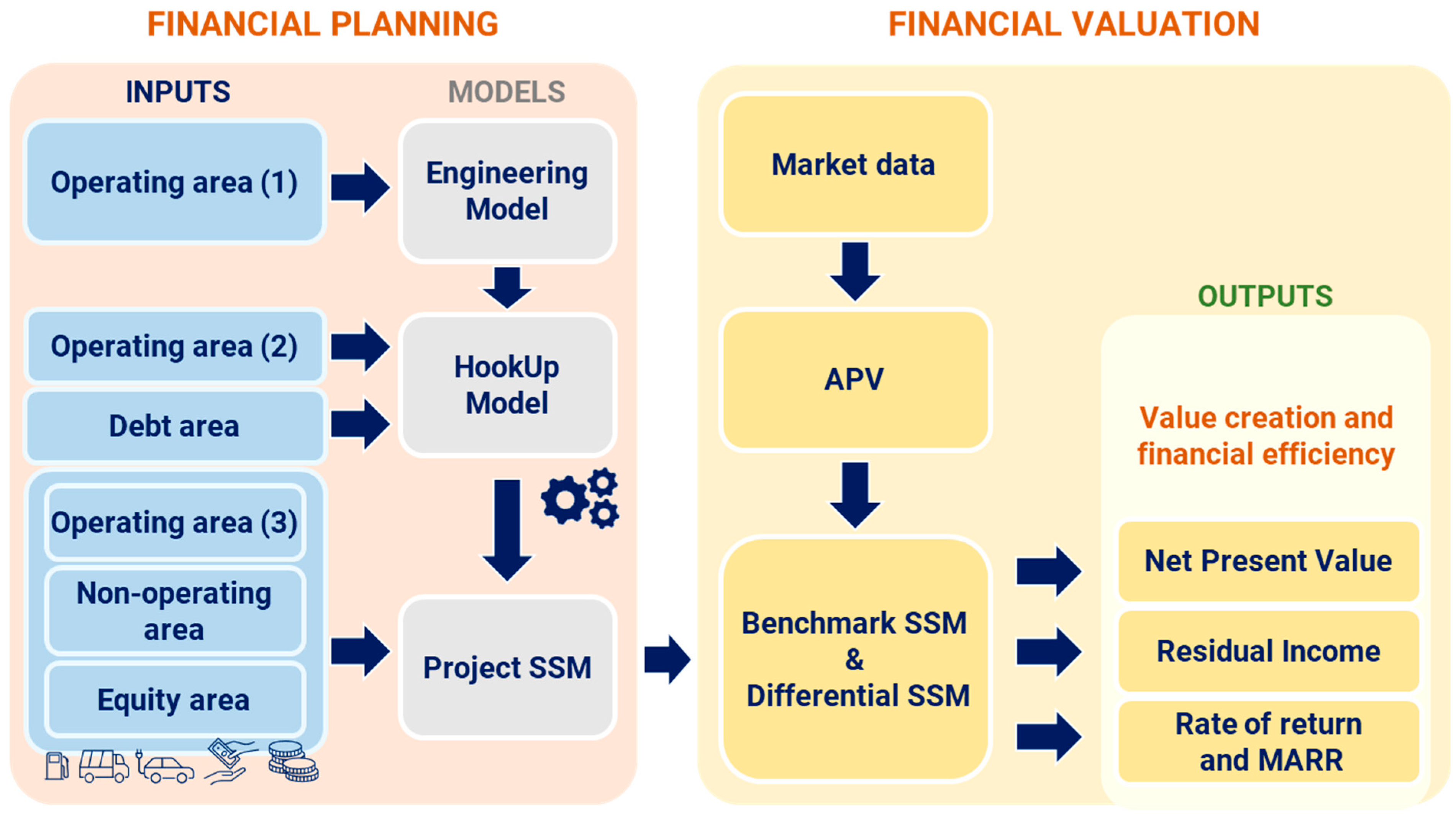
Figure 1 outlines the architecture of the system. We can easily identify the three main blocks:

(1)

“Inputs”: containing all the problem input data,

(2)

“Models”: processing data from both engineering and financial perspectives,

(3)

“Outputs”: presenting the final summarized values, crucial for evaluating projects and aiding decision-making.

In the first block, the inputs belong to five classes, based on the financial magnitude they affect:

(i)

the class of operating inputs, broken down to three classes, according to the model that processes them (Engineering model, HookUp model, Financial model),

(ii)

the class of debt inputs, consisting of data relating to borrowing to cover the capital expenditures (CapEx),

(iii)

the class of non-operating inputs, related to the reinvestment of cash flows generated by the project and not distributed to Iren Ambiente’s shareholders,

(iv)

the class of equity inputs, consisting of one input, the payout ratio, calculated on the project’s net incomes of the previous year,

(v)

the class of market data, used for estimating the costs of capital (i.e., the minimum attractive rates for each one of the above-mentioned area).

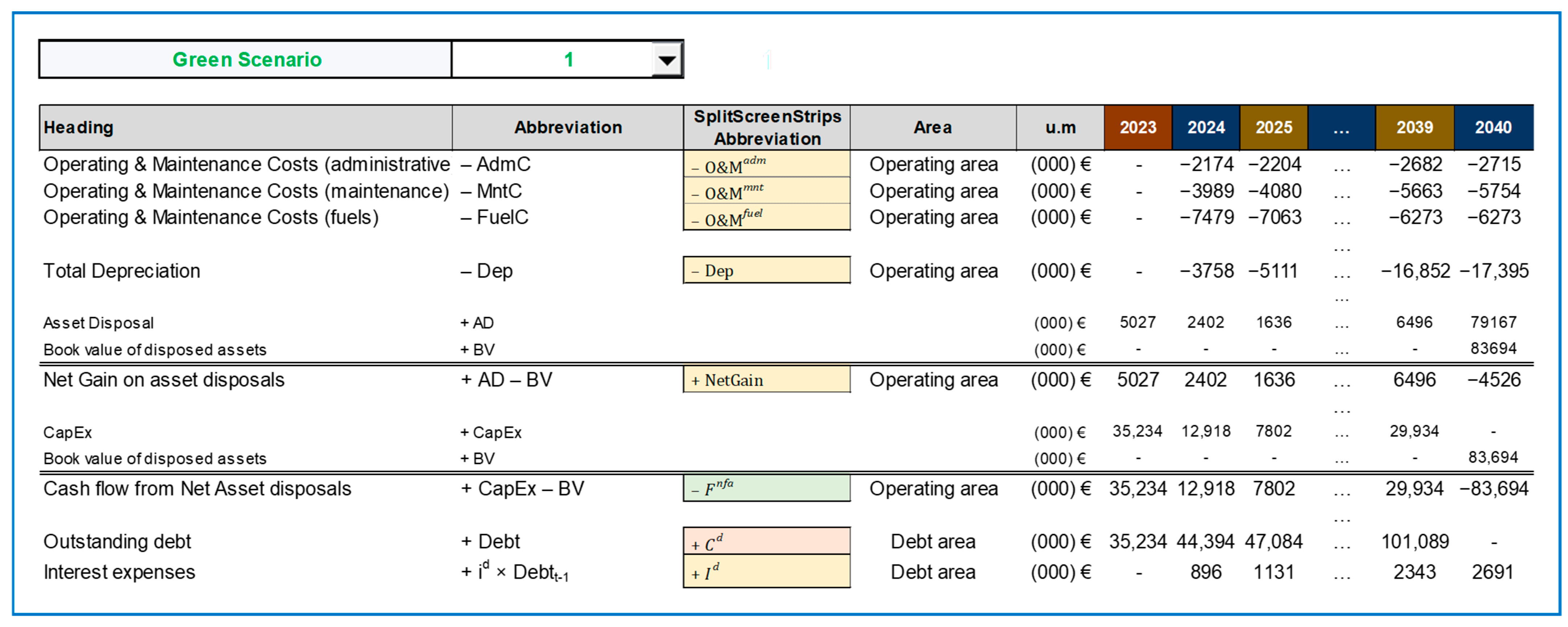
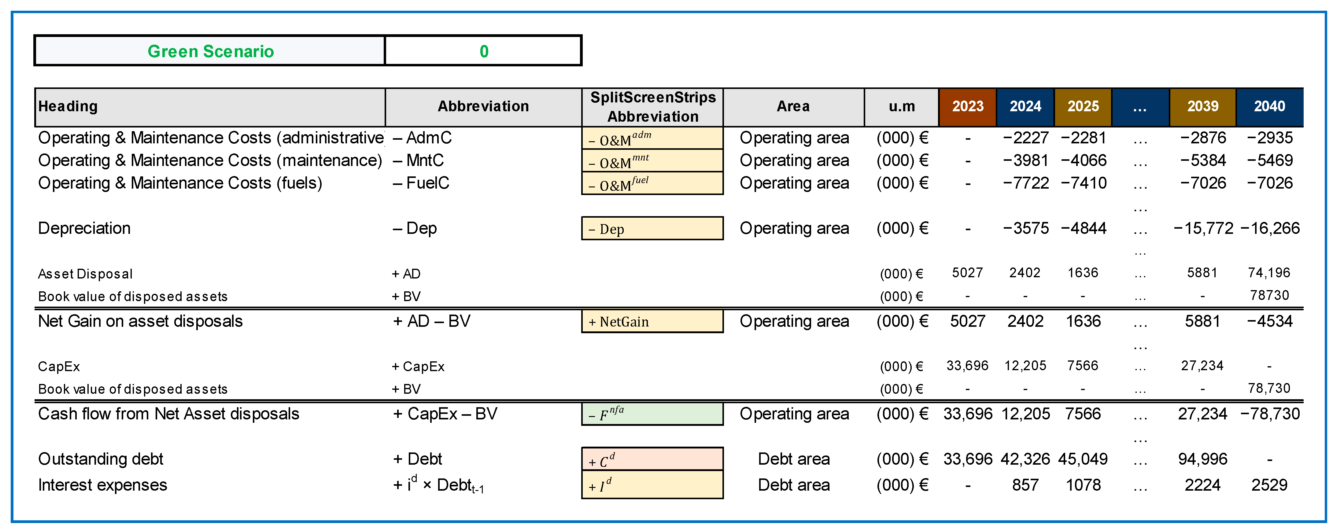
The first set of inputs undergo processing within the Engineering model. Subsequently, the Engineering model outputs, together with additional operating inputs and the inputs related to the debt area, proceed to the HookUp model. This model transforms the five scenarios into five projects and produces a range of accounting outputs for the five projects, encompassing operating and maintenance costs, depreciation, gains and losses on asset disposals, CapEx, cash flow from net asset disposals, outstanding debt, and interest expenses.

The Financial model employs the outputs generated by the HookUp model along with the remaining inputs. It processes these combined data and organizes them into pro forma financial statements (presented as a strip of Split-Screen Matrices), whence the financial evaluation is obtained, with NPVs, rates of return, and financial efficiencies. Then, we concentrate on the NPV and the NGV, directly derived from the Engineering model. Plotting the five NPV-NGV pairs on an xy-plane, we obtain the main output of the whole system: the Net Value curve. This curve represents a Pareto frontier, balancing the trade-off between the NPV and the NGV.

4. Problem Inputs

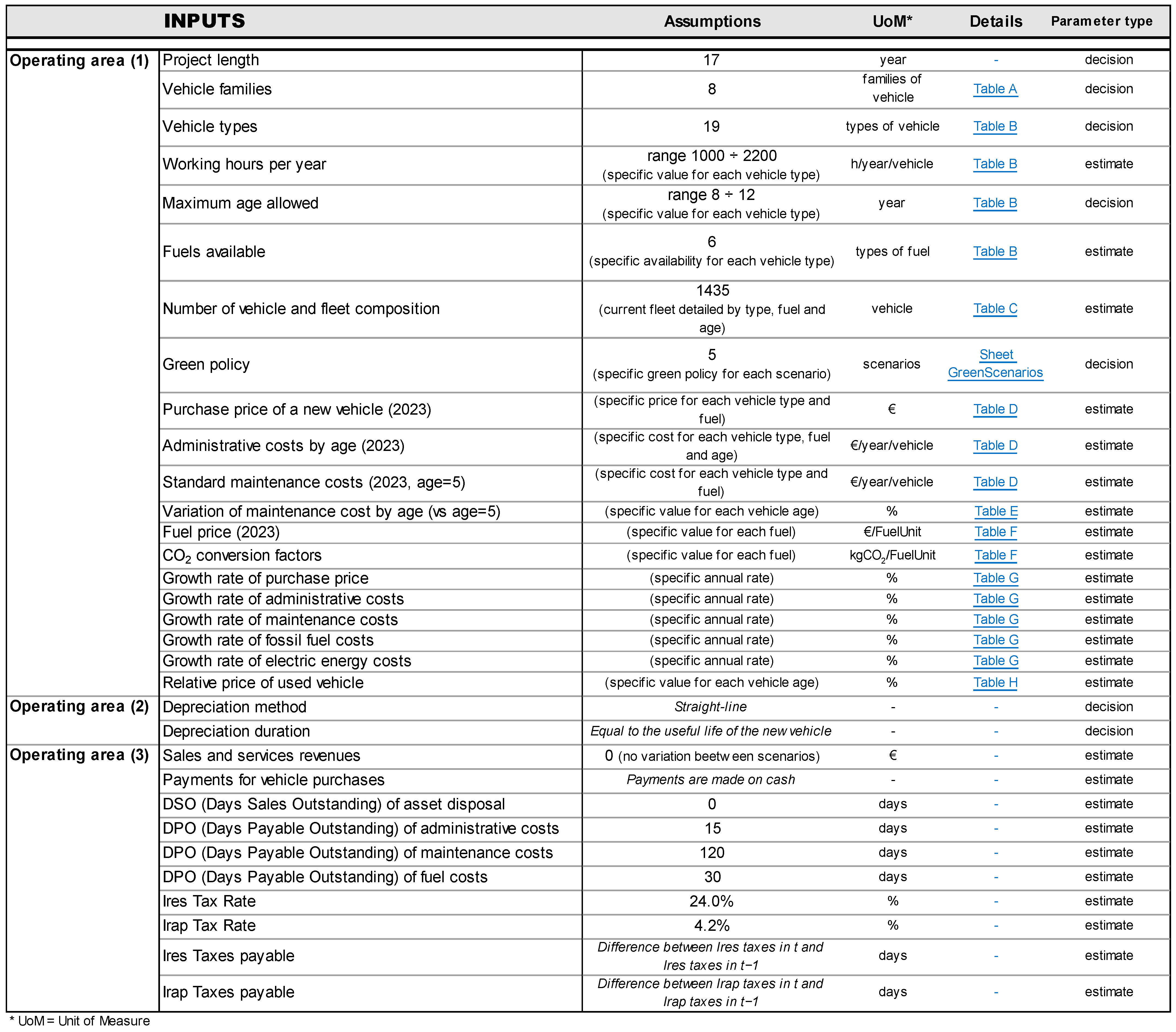
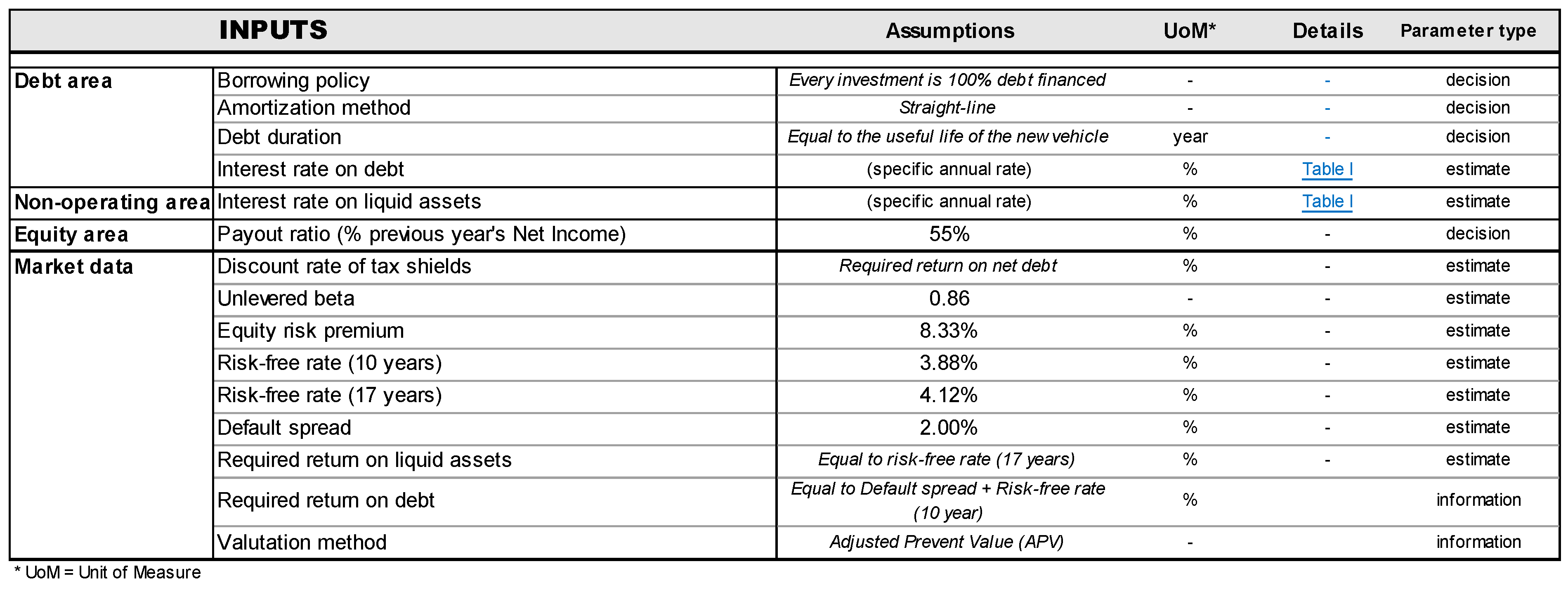
In total, we have managed 2303 inputs (see Figure 2 and Figure 3): most of them are quantitative inputs with a few qualitative inputs (e.g., vehicle families or types, depreciation method, debt amortization method). This means that the size of the problem is substantial, posing significant computational complexity in logical and computational terms. Inputs are categorized as either “estimate” or “decision” variables and are segmented into five areas: operating, debt, non-operating, equity, and market data.3 The operating inputs are broken down into three classes, according to the model that processes them: some feed into the Engineering model, some into the HookUp model, and others into the Financial model (see Figure 1 and Figure A1 in the Appendix A).4 The inputs within the operating area undergo a nontrivial processing, determining the policy of vehicle replacement and the annual composition of the fleet, and, hence, impacting on Iren Ambiente’s operating assets, operating income, and operating cash flow. The inputs in the debt area pertain to Iren Ambiente’s borrowing policy to finance the acquisition of new vehicles. The inputs of the equity and non-operating areas relate to Iren Ambiente’s payout policy affecting the amount of cash flow distributed to equityholders and, consequently, the amount of cash flow retained in the firm. The market data inputs provide estimates for the costs of capital, specifically the required return on operating assets (unlevered cost of assets), the required return on non-operating (liquid) assets, and the required return on debt. All assumptions have been made with the assistance of Iren Ambiente’s engineers and executives or inferred from IREN’s internal documents (e.g., the payout ratio).

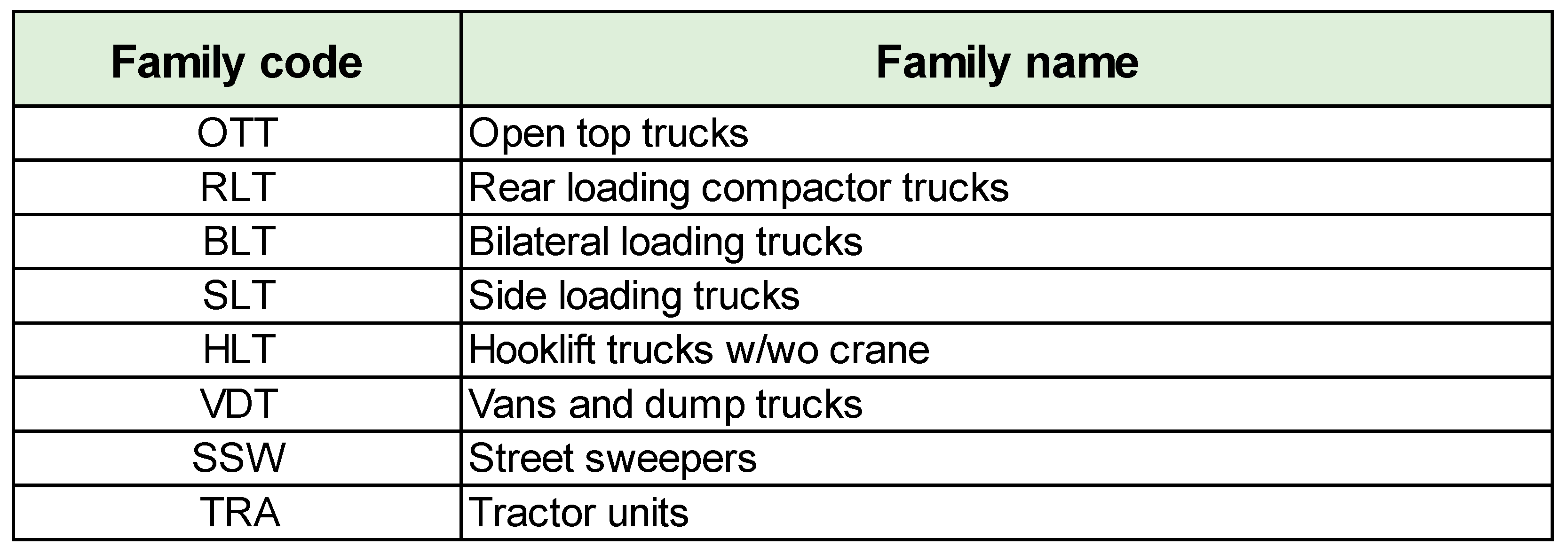
Operating inputs. The 2244 inputs of the operating area are used for the determining the accounting and financial magnitudes of the five project’s operating assets, corresponding to the five green scenarios. They include the project length, equal to 17 years (year 2023 to year 2040). The choice is motivated by IREN’s explicit request of representing a medium- to long-term outlook, sufficient to observe more than one vehicle renewal cycle. In particular, in accordance with IREN’s planning practices, we use the end of the decade as the time horizon (i.e., 2040). The problem focuses on the analysis of the 8 main vehicle families in use in the waste collection sector: open top trucks, rear loading compactor trucks, bilateral loading trucks, slide loading trucks, hooklift trucks with or without crane, vans and dump trucks, street sweepers, and tractor units (Figure A2) (see Note 4). Each family is associated with a family code. Each family is broken down into several vehicle types, which differ in equipment type and/or size (gross vehicle weight, GVW, for collection or transport vehicles, and volume for sweepers). In our problem, there are 19 vehicle types, identified by progressive IDs; for each vehicle type, we define the working hours per year, the maximum age allowed by IREN’s operating practices, and the types of fuel available when purchasing new vehicles (Figure A3). These data were provided by Iren Ambiente’s Fleets and Equipment sector. The starting fleet of our problem has 1435 vehicles. They are part of the fleet of the Environment Business Unit of the IREN Group as of 31 December 2022. Following the principles used by IREN and described in Section 3, the problem involves the evaluation and comparison of multiple scenarios, defined by increasing degree of environmental sustainability. Scenario 0 (status quo) corresponds to the no-green policy: each vehicle is replaced with a new one of the same type and same fuel (this is the current replacement policy by Iren Ambiente). With the assistance of IREN’s technical departments, we have defined five alternative green scenarios, from a very cautious one to a very challenging one, whereby each vehicle is replaced with a new one of the same type but equal or different fuel, depending on the scenario (Figure 4).

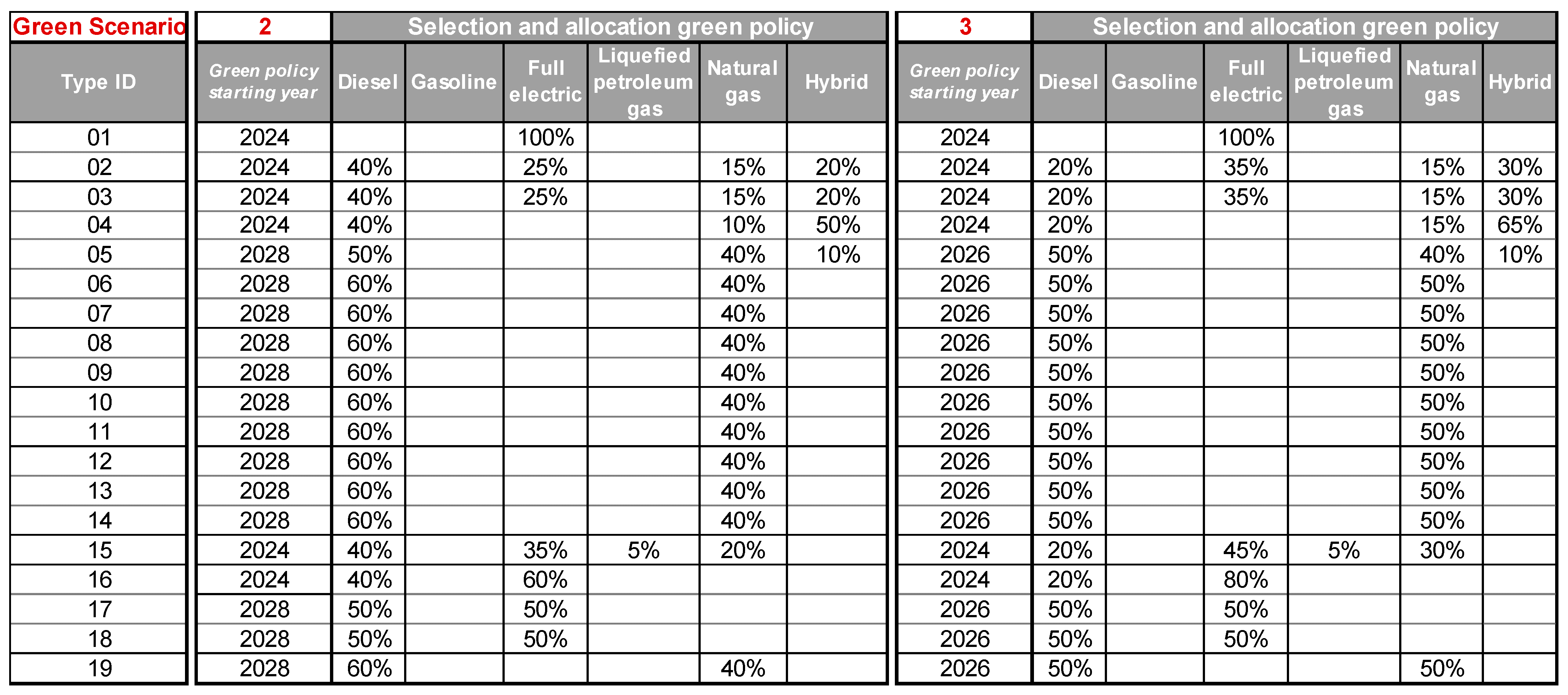
For each scenario and for each vehicle type, a starting year is defined: before this year, vehicles are replaced with a new vehicle of the same type and fuel; from the starting year onward, purchases of new vehicles follow the selected vehicle replacement policy (Figure A4 and Figure A5 and Figure 5 below). For example, consider Scenario 4 in Figure 5. If we consider the medium-rear-loading compactor trucks (Type ID = 05), the 2024 and 2025 purchases for this type of vehicle will have the same fuel as the disposed vehicles; from 2026 onward, the allocation of purchases will follow the (time-invariant) percentages 50% diesel, 40% natural gas, and 10% hybrid.

In collaboration with IREN’s technical departments, we have estimated (i) the purchase price of a new vehicle, (ii) the administrative costs (by age of vehicle), (iii) the standard maintenance costs, (iv) the hourly fuel consumption, from which the annual fuel cost/emissions will be derived as a product of hourly fuel consumption, working hours per year, and unit fuel price/CO₂ conversion factor (Figure A6).5

Figure A7 shows the annual growth rates of purchase prices of vehicles, the administrative costs, the maintenance costs, the fossil fuel costs (diesel, gasoline, liquefied petroleum gas, natural gas) and electricity costs. To make such forecasts, we have relied on estimates made by IREN’s experienced executives, who have a robust knowledge of both the waste collection sector and the energy market. In particular, Iren Energia Spa, a subsidiary of IREN Group, has an area dedicated to short-, medium- and long-term forecasts of market prices.

Some operating inputs feed the HookUp model. They include the depreciation method (Iren Ambiente’s vehicles are depreciated with the straight-line depreciation method) and the depreciation duration (the years of depreciation of a vehicle coincide with the useful life of the new vehicle).

Other operating inputs feed the Financial model:

(i)

Payments for vehicle purchase (made on a cash basis, so accounts payable for vehicle supplies are zero in each year); the payments are covered by loans, granted by the parent company (Iren Spa),

(ii)

Days Sales Outstanding of asset disposals (estimated to be zero, since, in the sale of used vehicles, payments are nearly immediate),

(iii)

Days Payable Outstanding of administrative costs, maintenance costs, and fuels costs (calculated according to average values estimated by IREN’s Management Control System),

(iv)

Taxes (Ires tax and Irap tax).

Debt inputs. The inputs of the debt area serve the scope of determining the debt, the interest rate on debt, and the cash flow to debt. They concern the borrowing policy for purchases of new vehicles and can be divided into (i) borrowing policy: every new investment in vehicles is 100% debt financed (funds are borrowed from the parent company, Iren Spa), (ii) amortization method: it matches the depreciation method for vehicles (i.e., straight-line amortization), (iii) debt duration: debt is equal to the maximum age allowed for the new vehicle, (iv) the interest rate on debt (the annual rate is defined for each year of the plan). The estimates for the years 2023 to 2030 have been provided by the IREN Group finance area (Figure A8, upper block). For the remaining years, the interest rates are estimated to be equal to the average interest rate on debt recorded in the 2023–2030 timeframe (Figure A8, lower block).

Non-operating inputs. The only input of the non-operating area is the interest rate on liquid assets. This is the rate of return of the amount of operating cash flow generated by the project that is retained by the firm, that is, not distributed to the equityholders (Figure A8). Investments in liquid assets are managed by the parent company, Iren Spa. The values from 2023 to 2030 have been provided by the IREN Group finance area, while for the later years they are assumed to be equal to the average interest rate on liquid assets in the span 2023–2030. These values are necessary to calculate the balance of liquid assets in the pro forma financial statements.

Equity inputs. The only input of the equity area is the payout ratio. It expresses the dividend policy, defined as the percentage of previous year’s net income allocated to equityholders. The payout ratio is estimated to be 55%, midpoint of the 50–60% range, which is the forthcoming payout ratio in the next years, as publicly communicated by IREN.

Market data. The market data refer to the costs of capital (required returns). They are necessary to calculate the NPV of each project and the NPV of each project’s area (operating, non-operating, equity, and debt). Specifically, the unlevered cost of assets (k^u) is necessary to determine the operating value (and NPV) of the projects. It represents the minimum attractive rate of return (MARR) that justifies the project undertaking. Using the Capital Asset Pricing Model (Sharpe, 1964; Mossin, 1966), its calculation depends on the unlevered beta, the equity risk premium, and the risk-free rate: we use the estimates reported on the widely respected website of Prof. Aswath Damodaran (https://pages.stern.nyu.edu/~adamodar/New_Home_Page/home.htm, accessed on 20 November 2023), for the unlevered beta and the equity risk premium for the Environmental & Waste Services industry, and use the Italian 17-year government bond as a proxy for the risk-free rate. Since reinvestment in liquid assets will be essentially riskless, we use this rate as a proxy for the required return on liquid assets as well. For calculating the required return on debt, we sum the 10-year return on government bonds and the default spread for IREN, based on the BBB rating recently made by Standard & Poor’s.

5. Engineering Model

The Engineering model comprises 15 worksheets in the Excel file and serves the purpose of processing the operating inputs, generating a series of intermediate outputs. These outputs will undergo further processing in the HookUp model before being transmitted to the Financial model. The Engineering Model specifically calculates the annual evolution of the fleet based on the chosen green scenario and the operating inputs. 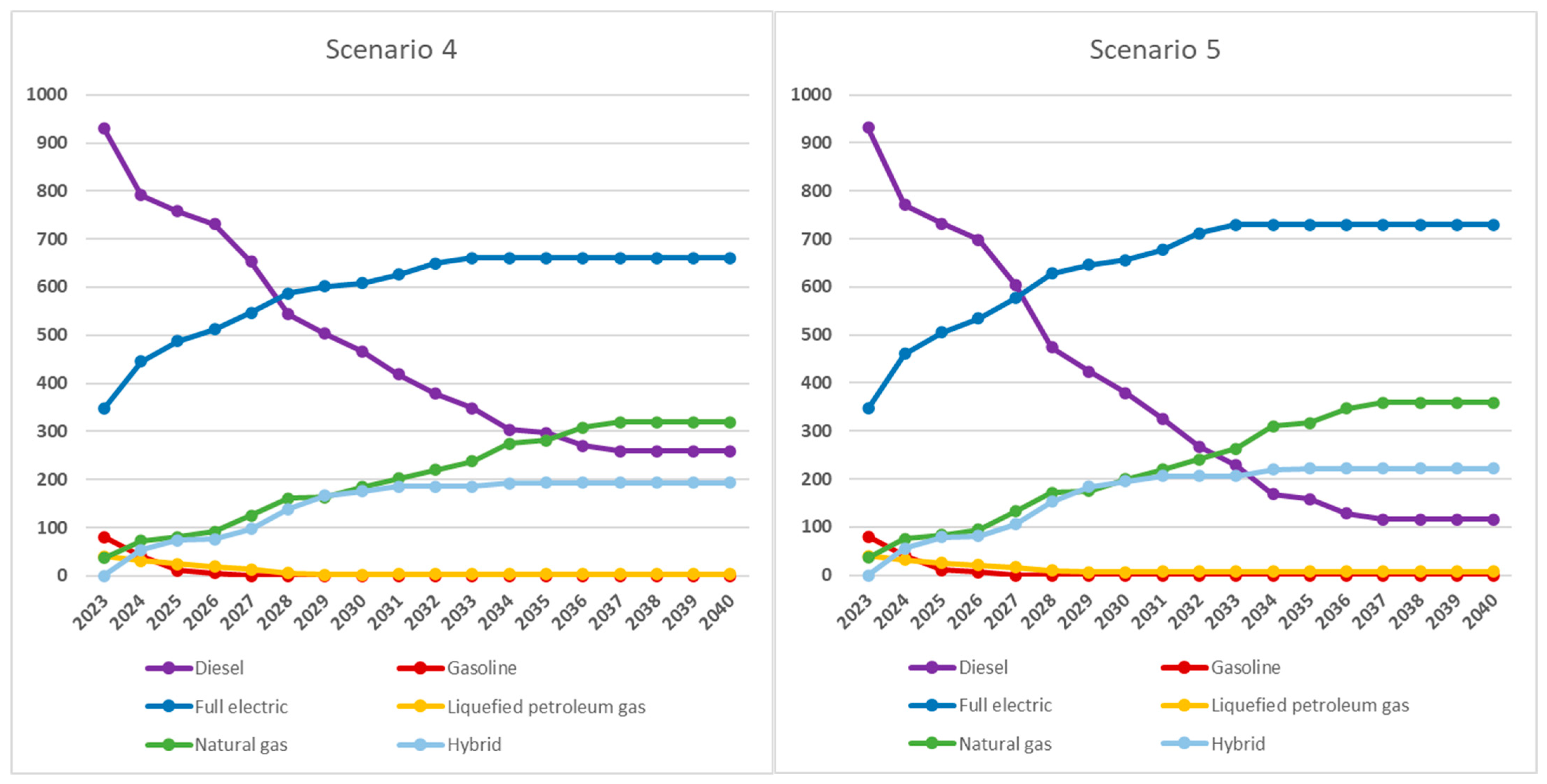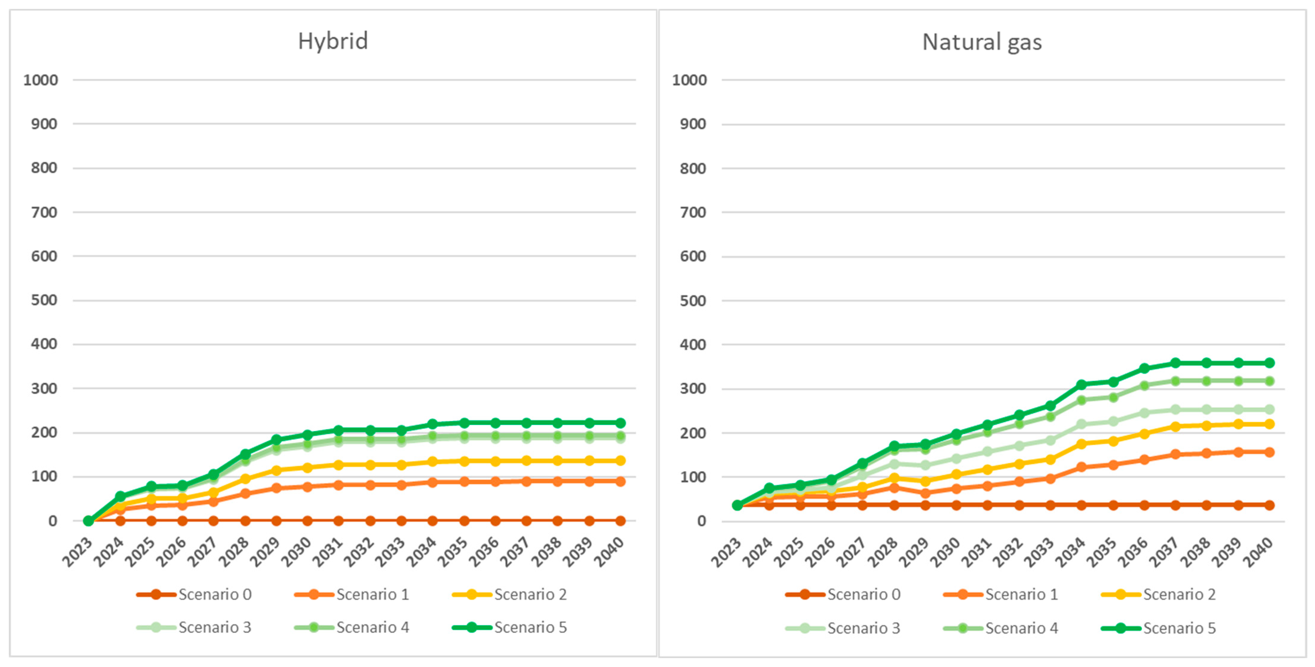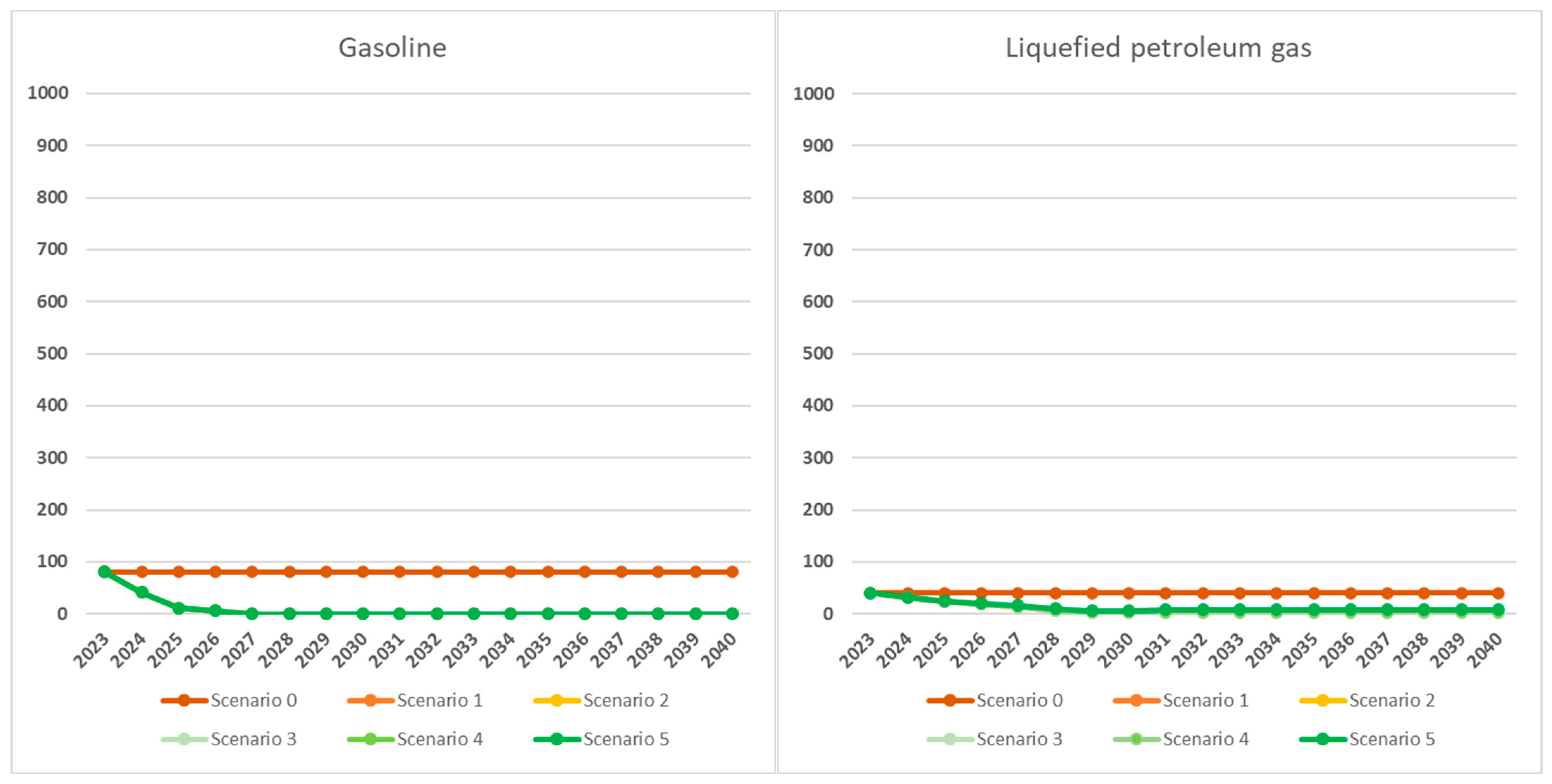Figure A9, Figure A10 and Figure A11 show the resulting fleet composition for each year across the five green scenarios analyzed. It is evident that the fleet undergoes a progressive shift towards greater environmental friendliness, with a decreasing incidence of diesel and gasoline vehicles in favor of electric, hybrid, and natural gas vehicles. 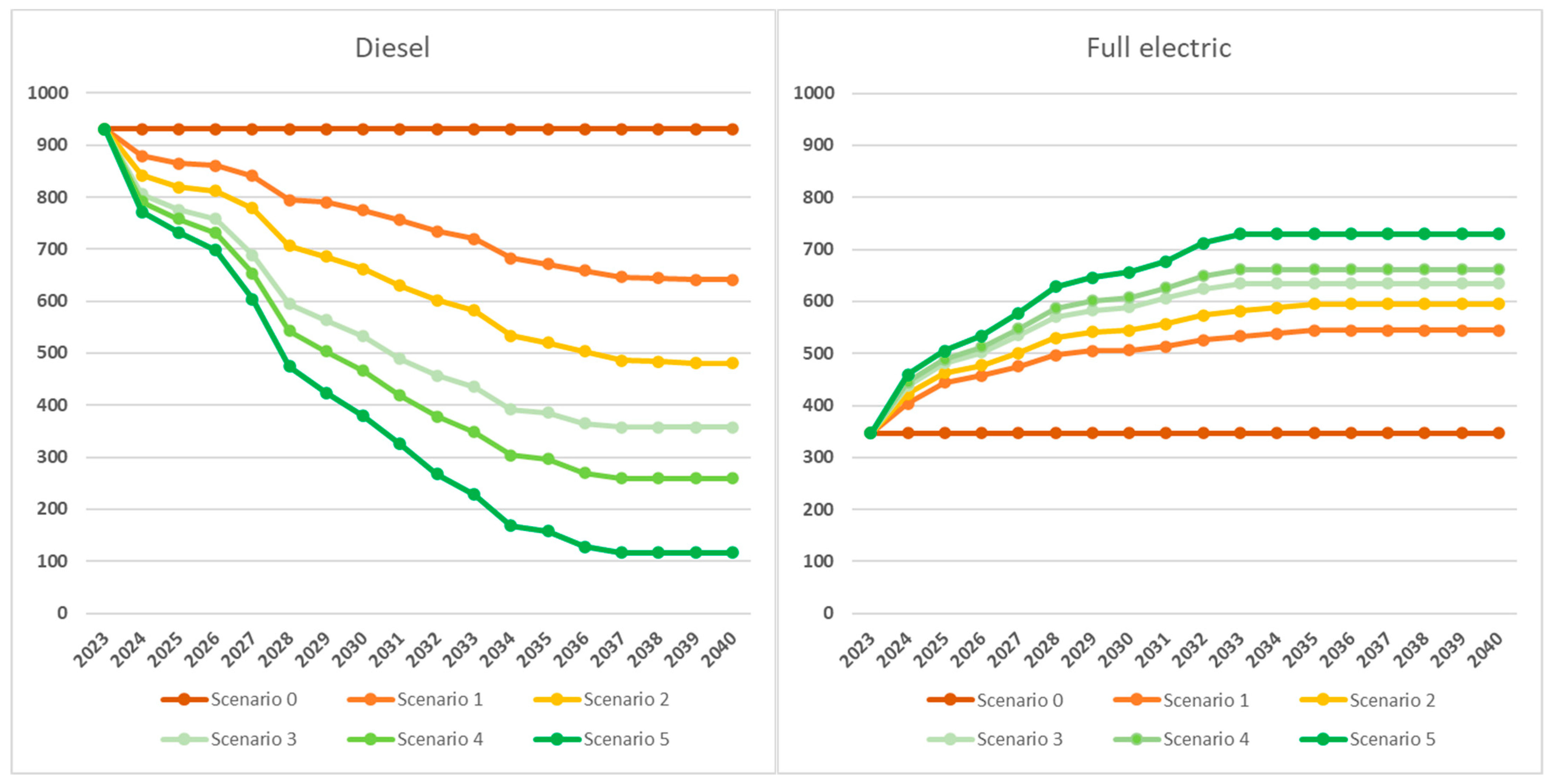In Figure 6, Figure 7 and Figure 8, we show, for each fuel type, the evolution over the years of the number of vehicles expected in the different scenarios. We note that

• for diesel, the curves clearly decline when compared with the status quo (scenario 0, constant fleet composition) as scenarios become greener;
• for gasoline and LPG (non-green fuels), the decreasing trend is somewhat obscured by the limited number of existing vehicles in the initial phase (2023), which will be almost entirely decommissioned with approximately identical planning in all five green scenarios;
• for full electric, hybrid, and natural gas, the numbers of vehicles, will increase over time, compared with the status quo, with increasingly higher curves for greener scenarios. However, not even the greenest scenario (Scenario 5) involves a total conversion of all vehicles to green fuels (full electric, hybrid, and natural gas), let alone to only electric vehicles. The reason is that part of IREN’s case study fleet operates in territories where even in the medium term, a portion of diesel vehicles will be required, due to orographic and/or refueling or recharging infrastructure limitations. Also, for some vehicle types, the greenest applicable fuel is natural gas (e.g., for heavy truck and tractor units).

Figure A12 presents a summary of vehicle transactions for the year 2023 in Scenario 1. The figure indicates purchases with a plus sign and disposals with a negative sign. In this scenario, the 41 light open trucks of various ages and fuel owned by the company are disposed of and replaced by 41 full-electric new (0 age) light open trucks.

In this model, we calculate the growth factors ($\mathrm{G}\mathrm{F}$) of (i) purchase price, (ii) administrative costs, (iii) maintenance costs, (iv) fossil fuel costs, (v) electric energy costs, using the standard formula ${\mathrm{G}\mathrm{F}}_t={\mathrm{G}\mathrm{F}}_{t-1}·\left(1+{\mathrm{G}\mathrm{R}}_t\right)$ where ${\mathrm{G}\mathrm{R}}_t$ denotes the growth rate and ${\mathrm{G}\mathrm{F}}_0=1$. Then, we calculate

• the unit fuel costs from 2024 to 2040 by applying the respective growth rates to the unit fuel costs in 2023
• the purchase price ($\mathrm{P}\mathrm{P}$) of a new vehicle in each year $t$, using purchase prices of previous years and the growth rate for purchase prices ($\mathrm{G}\mathrm{R}\mathrm{P}\mathrm{P}$):

  $$\mathrm{P}{\mathrm{P}}_t=\mathrm{P}{\mathrm{P}}_{t-1}\times (1+\mathrm{G}\mathrm{R}\mathrm{P}{\mathrm{P}}_t)$$
• the maintenance costs ($\mathrm{M}\mathrm{n}\mathrm{t}\mathrm{C}$) by age ($a$) in 2023, using the inputted maintenance cost for 5-year-old vehicles, and the variation in maintenance costs ($\mathrm{V}\mathrm{a}\mathrm{r}\mathrm{M}\mathrm{n}\mathrm{t}\mathrm{C}$) from baseline age (5 years), as

  $${\mathrm{M}\mathrm{n}\mathrm{t}\mathrm{C}}_{2023,a}={\mathrm{M}\mathrm{n}\mathrm{t}\mathrm{C}}_{2023,a=5}\times (1+{\mathrm{V}\mathrm{a}\mathrm{r}\mathrm{M}\mathrm{n}\mathrm{t}\mathrm{C}}_a)$$
• the maintenance costs by age in each year, using the maintenance costs by age (2023), calculated as above, and the growth rate for Maintenance costs ($\mathrm{G}\mathrm{R}\mathrm{M}\mathrm{n}\mathrm{t}\mathrm{C}$):

  $${\mathrm{M}\mathrm{n}\mathrm{t}\mathrm{C}}_{t,a}={\mathrm{M}\mathrm{n}\mathrm{t}\mathrm{C}}_{t-1,a}\times (1+{\mathrm{G}\mathrm{R}\mathrm{M}\mathrm{n}\mathrm{t}\mathrm{C}}_t)$$
• the administrative costs ($\mathrm{A}\mathrm{d}\mathrm{m}\mathrm{C}$) by age in each year, using the inputted administrative costs by age (2023) and growth rate for administrative costs ($\mathrm{G}\mathrm{R}\mathrm{A}\mathrm{d}\mathrm{m}\mathrm{C}$):

  $${\mathrm{A}\mathrm{d}\mathrm{m}\mathrm{C}}_{t,a}={\mathrm{A}\mathrm{d}\mathrm{m}\mathrm{C}}_{t-1,a}\times (1+{\mathrm{G}\mathrm{R}\mathrm{A}\mathrm{d}\mathrm{m}\mathrm{C}}_t)$$
• the annual fuel consumption of each type of vehicle and fuel, computed as the product of the inputted working hours per year and the hourly fuel consumption (we assume that the annual consumption is not age-dependent, because the estimated maintenance costs are such that the vehicle’s efficiency remains constant):

  $$\begin{array}{c}\mathrm{A}\mathrm{n}\mathrm{n}\mathrm{u}\mathrm{a}\mathrm{l}\\ \mathrm{f}\mathrm{u}\mathrm{e}\mathrm{l} \mathrm{c}\mathrm{o}\mathrm{n}\mathrm{s}\mathrm{u}\mathrm{m}\mathrm{p}\mathrm{t}\mathrm{i}\mathrm{o}\mathrm{n}\end{array}=\left(\begin{array}{c}\mathrm{W}\mathrm{o}\mathrm{r}\mathrm{k}\mathrm{i}\mathrm{n}\mathrm{g} \mathrm{h}\mathrm{o}\mathrm{u}\mathrm{r}\mathrm{s}\\ \mathrm{p}\mathrm{e}\mathrm{r} \mathrm{y}\mathrm{e}\mathrm{a}\mathrm{r}\end{array}\right)\times \left(\begin{array}{c}\mathrm{H}\mathrm{o}\mathrm{u}\mathrm{r}\mathrm{l}\mathrm{y} \mathrm{f}\mathrm{u}\mathrm{e}\mathrm{l}\\ \mathrm{c}\mathrm{o}\mathrm{n}\mathrm{s}\mathrm{u}\mathrm{m}\mathrm{p}\mathrm{t}\mathrm{i}\mathrm{o}\mathrm{n}\end{array}\right)$$
• the fuel costs ($\mathrm{F}\mathrm{u}\mathrm{e}\mathrm{l}\mathrm{C}$), by type of vehicle and fuel in each year, is calculated using the annual fuel consumption, computed as above, and the unit fuel costs from 2024 to 2040:

  $${\mathrm{F}\mathrm{u}\mathrm{e}\mathrm{l}\mathrm{C}}_t=\left(\begin{array}{c}\mathrm{A}\mathrm{n}\mathrm{n}\mathrm{u}\mathrm{a}\mathrm{l}\\ \mathrm{f}\mathrm{u}\mathrm{e}\mathrm{l} \mathrm{c}\mathrm{o}\mathrm{n}\mathrm{s}\mathrm{u}\mathrm{m}\mathrm{p}\mathrm{t}\mathrm{i}\mathrm{o}\mathrm{n}\end{array}\right)\times \mathrm{U}\mathrm{n}\mathrm{i}\mathrm{t}\mathrm{F}\mathrm{u}\mathrm{e}\mathrm{l}\mathrm{C}\mathrm{o}\mathrm{s}{\mathrm{t}}_t$$
• the annual CO₂ emissions of each type of vehicle and fuel, obtained as the product of annual fuel consumption, calculated as above, and the CO₂ conversion factor:

  $$\begin{array}{c}\mathrm{A}\mathrm{n}\mathrm{n}\mathrm{u}\mathrm{a}\mathrm{l}\\ \mathrm{C}{\mathrm{O}}_2 \mathrm{e}\mathrm{m}\mathrm{i}\mathrm{s}\mathrm{s}\mathrm{i}\mathrm{o}\mathrm{n}\mathrm{s}\end{array}=\left(\begin{array}{c}\mathrm{A}\mathrm{n}\mathrm{n}\mathrm{u}\mathrm{a}\mathrm{l}\\ \mathrm{f}\mathrm{u}\mathrm{e}\mathrm{l} \mathrm{c}\mathrm{o}\mathrm{n}\mathrm{s}\mathrm{u}\mathrm{m}\mathrm{p}\mathrm{t}\mathrm{i}\mathrm{o}\mathrm{n}\end{array}\right)\times \left(\begin{array}{c}\mathrm{C}{\mathrm{O}}_2\\ \mathrm{c}\mathrm{o}\mathrm{n}\mathrm{v}\mathrm{e}\mathrm{r}\mathrm{s}\mathrm{i}\mathrm{o}\mathrm{n} \mathrm{f}\mathrm{a}\mathrm{c}\mathrm{t}\mathrm{o}\mathrm{r}\end{array}\right)$$
• the disposal values ($\mathrm{D}\mathrm{i}\mathrm{s}\mathrm{p}\mathrm{V}$) of a used vehicle in each year are calculated as the product of the purchase price ($\mathrm{P}\mathrm{P}$) of an equivalent new vehicle in that year and the percentage of relative price of a used vehicle of that age (found in Figure A13):

  $${\mathrm{D}\mathrm{i}\mathrm{s}\mathrm{p}\mathrm{V}}_{t, a}={\mathrm{P}\mathrm{P}}_t\times \mathrm{R}\mathrm{e}\mathrm{l}\mathrm{a}\mathrm{t}\mathrm{i}\mathrm{v}\mathrm{e} \mathrm{C}\mathrm{o}\mathrm{s}\mathrm{t} \mathrm{f}\mathrm{o}\mathrm{r} \mathrm{s}\mathrm{a}\mathrm{m}\mathrm{e} \mathrm{a}\mathrm{g}\mathrm{e}$$
• the total administrative costs for each year and for any given scenario: for all types of vehicles, we multiply the administrative cost of a single vehicle by age for each year and the number of vehicles by type, fuel, and age in each year
• the total maintenance costs and the total fuel costs (same procedure as for the total administrative costs)
• the total CapEx for each year, multiplying the purchase price of a single new vehicle by the corresponding number of purchased vehicles and then adding these up
• the total asset disposals (same procedure as above, with disposal values replacing purchase prices).

We also calculate the total CO₂ emission of the fleet in each year. For all types of vehicles (rows), first, we calculate the estimated emissions of CO₂ as the product of the annual CO₂ emissions of a single vehicle and the number of vehicles by type and fuel in each year. Then, adding these up, we obtain the total CO₂ emission of our fleet in each year.

6. HookUp Model

The HookUp model connects the Engineering model to the Financial model. It comprises two parts (corresponding to two sheets in the Excel file). The first part receives CapEx from the Engineering model and calculates the outstanding debt for each year and each scenario. The years of depreciation and the duration of debt are both equal to the useful life of the asset (i.e., maximum age allowed for the asset). The method of asset depreciation and debt amortization is straight-line, so that the depreciation charges and the principal repayments coincide; all asset purchases are 100% financed with debt. We calculate the following magnitudes:

• the total capital expenditure for each green scenario, classified by useful life of the vehicle (Figure A14)
• the annual depreciation charge for vehicles having a useful life equal to $ul$:

  $$\mathrm{D}\mathrm{e}\mathrm{p}\mathrm{r}\mathrm{e}\mathrm{c}\mathrm{i}\mathrm{a}\mathrm{t}\mathrm{i}\mathrm{o}\mathrm{n} {\mathrm{c}\mathrm{h}\mathrm{a}\mathrm{r}\mathrm{g}\mathrm{e}}_{t,ul}={\displaystyle \frac{\mathrm{C}\mathrm{a}\mathrm{p}\mathrm{E}{\mathrm{x}}_{t-1,ul}}{ul}}$$

  where $ul=8,10,12$ (Figure A15). For example, consider the depreciation charge of 19 thousand euros in year 2031 for vehicles with a useful life of eight years; since CapEx is in 2030 is 153 thousand euros, we apply the above equation with $t=2031$ and obtain

  $$\mathrm{D}\mathrm{e}\mathrm{p}\mathrm{r}\mathrm{e}\mathrm{c}\mathrm{i}\mathrm{a}\mathrm{t}\mathrm{i}\mathrm{o}\mathrm{n} {\mathrm{c}\mathrm{h}\mathrm{a}\mathrm{r}\mathrm{g}\mathrm{e}}_{\mathrm{2031,8}}={\displaystyle \frac{\mathrm{C}\mathrm{a}\mathrm{p}\mathrm{E}{\mathrm{x}}_{\mathrm{2030,8}}}{8}}= {\displaystyle \frac{153}{8}}=19.1$$

  (Figure A15, column 10, values in thousands of euros).
• the total depreciation for each year, adding up all the annual depreciation charges associated with the vehicles with useful life $ul$:

  $${\mathrm{T}\mathrm{o}\mathrm{t}\mathrm{a}\mathrm{l} \mathrm{d}\mathrm{e}\mathrm{p}\mathrm{r}\mathrm{e}\mathrm{c}\mathrm{i}\mathrm{a}\mathrm{t}\mathrm{i}\mathrm{o}\mathrm{n}}_{t,ul}=\sum _{k=t-ul+1}^{k=t}{\mathrm{D}\mathrm{e}\mathrm{p}\mathrm{r}\mathrm{e}\mathrm{c}\mathrm{i}\mathrm{a}\mathrm{t}\mathrm{i}\mathrm{o}\mathrm{n} \mathrm{c}\mathrm{h}\mathrm{a}\mathrm{r}\mathrm{g}\mathrm{e}\mathrm{s}}_{k,ul}$$

For example, the total depreciation of 5690 thousand euros in year 2031 for vehicles with a useful life of eight years is obtained as the sum of depreciation charges from year 2024 to year 2031 ($t-ul+1\le k\le t\to 2024\le k\le 2031$),

$$\begin{gathered} {\mathrm{T}\mathrm{o}\mathrm{t}\mathrm{a}\mathrm{l} \mathrm{d}\mathrm{e}\mathrm{p}\mathrm{r}\mathrm{e}\mathrm{c}\mathrm{i}\mathrm{a}\mathrm{t}\mathrm{i}\mathrm{o}\mathrm{n}}_{\mathrm{2031,8}} = \sum _{k=2024}^{k=2031}{\mathrm{D}\mathrm{e}\mathrm{p}\mathrm{r}\mathrm{e}\mathrm{c}\mathrm{i}\mathrm{a}\mathrm{t}\mathrm{i}\mathrm{o}\mathrm{n} \mathrm{c}\mathrm{h}\mathrm{a}\mathrm{r}\mathrm{g}\mathrm{e}\mathrm{s}}_{k,8} \\ = 1813+609+689+897+1235+305+124+19=5690 \end{gathered}$$

(Figure A15, columns 3–10, and Figure A16, column 10, values in thousands of euros).

• the outstanding debt:

  $${\mathrm{O}\mathrm{u}\mathrm{t}\mathrm{s}\mathrm{t}\mathrm{a}\mathrm{n}\mathrm{d}\mathrm{i}\mathrm{n}\mathrm{g} \mathrm{D}\mathrm{e}\mathrm{b}\mathrm{t}}_t={\mathrm{O}\mathrm{u}\mathrm{t}\mathrm{s}\mathrm{t}\mathrm{a}\mathrm{n}\mathrm{d}\mathrm{i}\mathrm{n}\mathrm{g} \mathrm{D}\mathrm{e}\mathrm{b}\mathrm{t}}_{t-1}-{\mathrm{P}\mathrm{r}\mathrm{i}\mathrm{n}\mathrm{c}\mathrm{i}\mathrm{p}\mathrm{a}\mathrm{l} \mathrm{r}\mathrm{e}\mathrm{p}\mathrm{a}\mathrm{y}\mathrm{m}\mathrm{e}\mathrm{n}\mathrm{t}\mathrm{s}}_t+{\mathrm{A}\mathrm{d}\mathrm{d}\mathrm{i}\mathrm{t}\mathrm{i}\mathrm{o}\mathrm{n}\mathrm{a}\mathrm{l} \mathrm{d}\mathrm{e}\mathrm{b}\mathrm{t}}_t$$

For example, the outstanding debt of 77,536 thousand euros in 2031 is calculated as the outstanding debt in 2030 minus the principal repayments in 2031 (equal to the total depreciation in 2031) plus the additional debt in 2031 (equal to the total CapEx in 2031):

$$\begin{gathered} {\mathrm{O}\mathrm{u}\mathrm{t}\mathrm{s}\mathrm{t}\mathrm{a}\mathrm{n}\mathrm{d}\mathrm{i}\mathrm{n}\mathrm{g} \mathrm{D}\mathrm{e}\mathrm{b}\mathrm{t}}_{2031}={\mathrm{O}\mathrm{u}\mathrm{t}\mathrm{s}\mathrm{t}\mathrm{a}\mathrm{n}\mathrm{d}\mathrm{i}\mathrm{n}\mathrm{g} \mathrm{D}\mathrm{e}\mathrm{b}\mathrm{t}}_{2030}-{\mathrm{P}\mathrm{r}\mathrm{i}\mathrm{n}\mathrm{c}\mathrm{i}\mathrm{p}\mathrm{a}\mathrm{l} \mathrm{r}\mathrm{e}\mathrm{p}\mathrm{a}\mathrm{y}\mathrm{m}\mathrm{e}\mathrm{n}\mathrm{t}\mathrm{s}}_{2031}+{\mathrm{N}\mathrm{e}\mathrm{w} \mathrm{d}\mathrm{e}\mathrm{b}\mathrm{t}}_{2031} \\ =\mathrm{65,995}-\mathrm{12,912}+\mathrm{24,453}=\mathrm{77,536} \end{gathered}$$

(Figure A17, columns 9 and 10, values in thousands of euros).

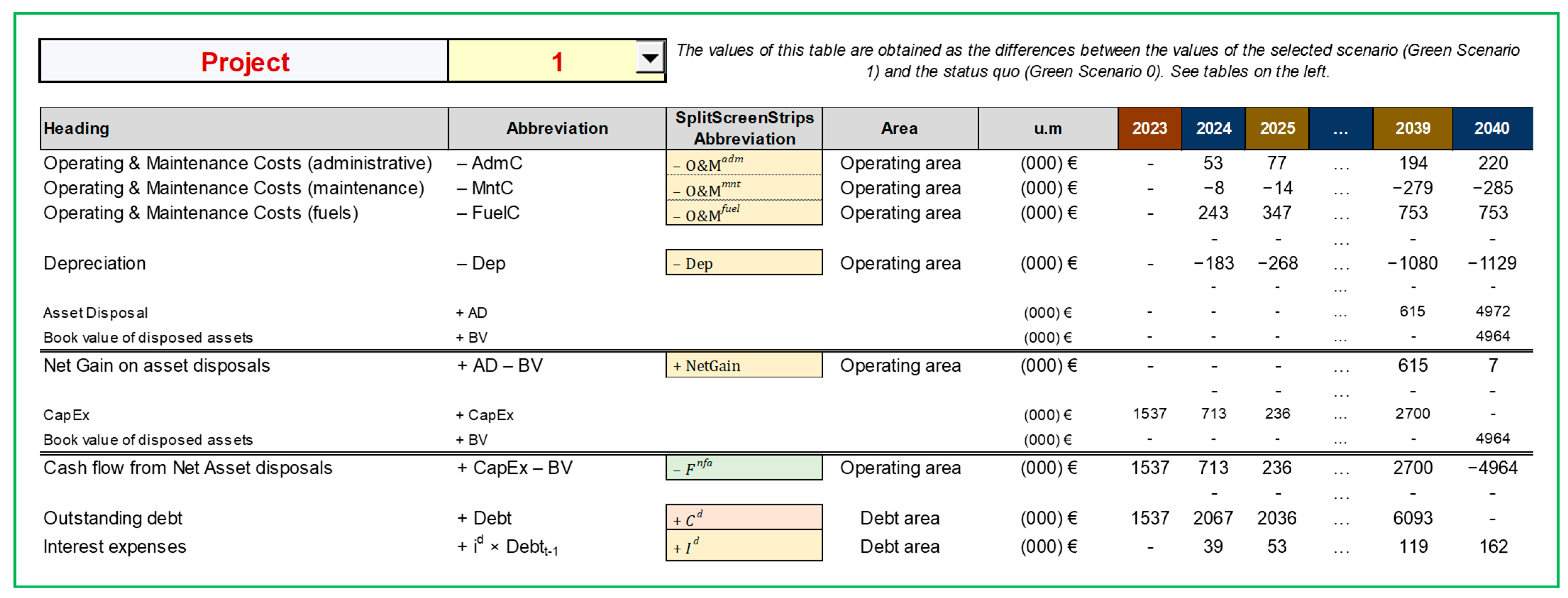
The second part of the HookUp model converts the five green scenarios processed by the Engineering model into five projects suitable for financial appraisal within the Financial model. This transition from an engineering to a financial perspective is essential and delicate. Specifically, a scenario represents a set of accounting magnitudes (e.g., costs, depreciation, capital expenditures, outstanding debt) under specific conditions. Scenario 0 is the status quo, where no change in the replacement policy occurs. Conversely, a project represents the financial effect of changing from the status quo (Scenario 0) to a specific alternative scenario (scenario $s\ne 0$). It is defined exclusively by the differential amounts, that is, the changes in each accounting magnitude relative to scenario 0.

This transformation process is accomplished by the HookUp model, which takes the accounting magnitudes for all scenarios ($s=0, 1, 2, 3, 4, 5$) and, for each alternative scenario ($s\ne 0$), calculates the differential amounts by subtracting Scenario 0 values from Scenario $s$ value. For example, if Scenario 0 has operating and maintenance costs (O&M) of USD 100, and Scenario $s\ne 0$ has O&M costs of USD 120, then the O&M cost for Project $s$ is the differential amounts of USD 20. This differential represents the incremental cost incurred by moving from Scenario 0 to Scenario $s$.

This transition from scenarios to projects is necessary: financial evaluation assesses the value created (or destroyed) by undertaking a specific change. A project, defined by these differential amounts, isolates the net financial effect of moving from the status quo (Scenario 0) to the target scenario $s\ne 0$. Only by analyzing the differential amounts can we calculate financial metrics such as the Net Present Value or the rate of return to evaluate the financial benefit of adopting Scenario $s$ over the status quo (see also Magni, 2020, Section 1.4, on the definition of a project). The HookUp model performs this essential conversion, enabling the Financial model to appraise the value created by each potential change (project).

Figure A18 reports an extract of accounting data regarding Project 1, obtained by subtracting the corresponding data of Scenario 1 (Figure A19) and Scenario 0 (Figure A20).

7. Financial Model

The Financial model is designed to manage both financial planning and financial valuation. Specifically, it

• generates the Balance Sheet, Income Statement, and Cash Flow Statement for each year and each project;
• calculates the NPV of each project (and each project’s area);
• determines the rate of return, the minimum attractive rate of return (MARR), and the financial efficiency of each project (and each project’s area).

This model comprises nine worksheets in the Excel file. They process the intermediate outputs received from the HookUp model along with the remaining inputs. The first 5 sheets conclude the financial planning of the projects, while the other four sheets focus on the financial valuation and analysis of the projects. The Financial model is theoretically grounded in the Split-Screen Approach developed by Magni (2020, 2023). This framework addresses severe limitations of conventional financial modeling by systematically integrating static accounting constructs with dynamic financial interdependencies through its innovative Split-Screen Matrix (SSM). The SSM aligns the Balance Sheet, Income Statement, and Cash Flow Statement within a unified structure based on two foundational principles: the law of motion, which governs capital dynamics via income and cash flows, and the law of conservation, which ensures equilibrium between investment and financing components. This matrix structure ensures internal consistency by modeling the horizontal (temporal) evolution capturing cross-statement flows, while preserving the vertical balance within each statement.

A distinctive feature of the SSA is its explicit incorporation of financing and payout decisions (often overlooked or excessively simplified in traditional models) and its generation of mutually consistent value metrics, such as the NPV, economic residual income, and project-specific rates of return. The model is implemented using basic spreadsheet functions, deliberately avoiding complex financial formulas to enhance transparency, error diagnosis, and scalability. These features make the SSA uniquely suited for large-scale projects where thousands of inputs interact dynamically across multi-year horizons. Unlike simplified models that obscure operational-financial linkages, the SSM offers diagnostic power to validate both dynamic and static dependencies between accounting variables and value drives. This closes a critical gap in the project appraisal literature and practice, while naturally bridging engineering and financial perspectives, making the SSA well suited for engineering-intensive contexts.

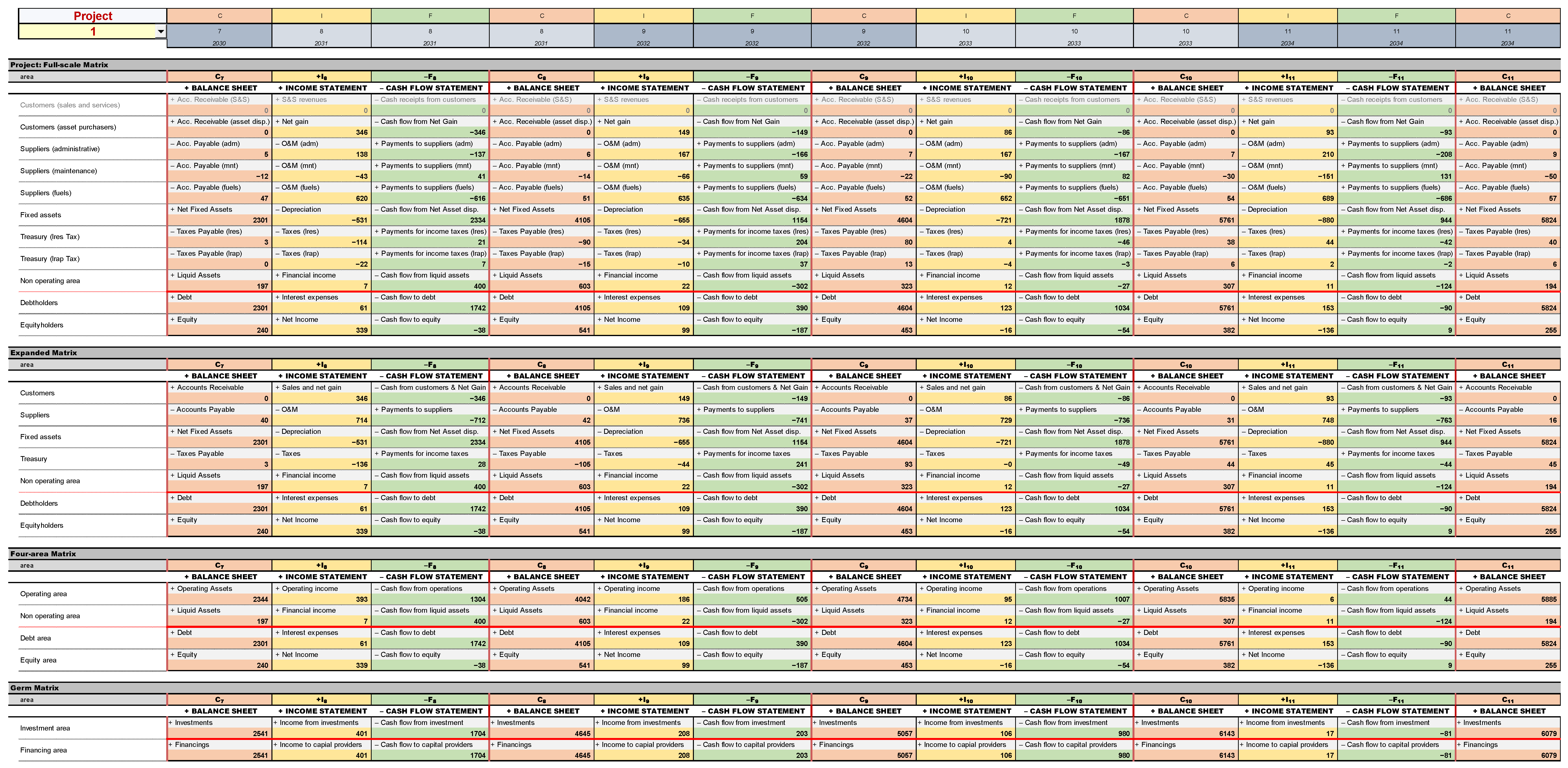
A sequence of consecutive SSMs, referred to as an SSM strip, displays the evolution of book values, incomes, and cash flows over all periods. The financial model consists of two SSM strips: the first one for the project (financial planning), and the other for the benchmark (financial valuation). Specifically, once the project SSM strip is established, the benchmark SSM strip is constructed, detailing the values, profits, and cash flows of benchmark portfolios replicating the project’s prospective cash flows. The projects’ financial valuation is obtained in the differential SSM, derived as the difference between project SSM and benchmark SSM. Within the differential SSM strip, one can find the NPV and the residual income (excess profit). For a better understanding, we reframe the architecture of our operations-and-finance system (Figure 1) in terms of financial planning and valuation, as illustrated in Figure 9. As can be gleaned by the figure, financial planning initiates with input data processed in the Engineering model. Utilizing the HookUp model and the remaining inputs, the project SSM is built, organizing all the accounting aspects for each year. As such, the project SSM marks the final stage step of financial planning. Subsequently, the project SSM and the market data are instrumental in accomplishing the financial valuation of the project using the Adjusted Present Value (APV) method. This valuation process involves establishing the benchmark SSM and then the differential SSM, enabling the derivation of relevant financial metrics: market value added, NPV, residual income, rate of return, minimum attractive rate of return (MARR) and, hence, financial efficiency.

Financial planning. Magni (2020, 2023) shows that the book value in year $t$ is linked to the balance sheet of the next year with the following law of motion:

$$\mathrm{B}\mathrm{o}\mathrm{o}\mathrm{k} {\mathrm{v}\mathrm{a}\mathrm{l}\mathrm{u}\mathrm{e}}_{t-1}+{\mathrm{I}\mathrm{n}\mathrm{c}\mathrm{o}\mathrm{m}\mathrm{e}}_t-{\mathrm{C}\mathrm{a}\mathrm{s}\mathrm{h} \mathrm{F}\mathrm{l}\mathrm{o}\mathrm{w}}_t=\mathrm{B}\mathrm{o}\mathrm{o}\mathrm{k} {\mathrm{v}\mathrm{a}\mathrm{l}\mathrm{u}\mathrm{e}}_t$$

Also, book values, incomes, and cash flows abide by the following law of conservation:

$$\mathrm{B}\mathrm{o}\mathrm{o}\mathrm{k} \mathrm{v}\mathrm{a}\mathrm{l}\mathrm{u}\mathrm{e} {\mathrm{o}\mathrm{f} \mathrm{i}\mathrm{n}\mathrm{v}\mathrm{e}\mathrm{s}\mathrm{t}\mathrm{m}\mathrm{e}\mathrm{n}\mathrm{t}\mathrm{s}}_t=\mathrm{B}\mathrm{o}\mathrm{o}\mathrm{k} \mathrm{v}\mathrm{a}\mathrm{l}\mathrm{u}\mathrm{e} {\mathrm{o}\mathrm{f} \mathrm{f}\mathrm{i}\mathrm{n}\mathrm{a}\mathrm{n}\mathrm{c}\mathrm{i}\mathrm{n}\mathrm{g}\mathrm{s}}_t$$

$$\mathrm{I}\mathrm{n}\mathrm{c}\mathrm{o}\mathrm{m}\mathrm{e} {\mathrm{f}\mathrm{r}\mathrm{o}\mathrm{m} \mathrm{i}\mathrm{n}\mathrm{v}\mathrm{e}\mathrm{s}\mathrm{t}\mathrm{m}\mathrm{e}\mathrm{n}\mathrm{t}\mathrm{s}}_t=\mathrm{I}\mathrm{n}\mathrm{c}\mathrm{o}\mathrm{m}\mathrm{e} \mathrm{t}\mathrm{o} \mathrm{c}\mathrm{a}\mathrm{p}\mathrm{i}\mathrm{t}\mathrm{a}\mathrm{l} {\mathrm{p}\mathrm{r}\mathrm{o}\mathrm{v}\mathrm{i}\mathrm{d}\mathrm{e}\mathrm{r}\mathrm{s}}_t$$

$$\mathrm{C}\mathrm{a}\mathrm{s}\mathrm{h} \mathrm{f}\mathrm{l}\mathrm{o}\mathrm{w} {\mathrm{f}\mathrm{r}\mathrm{o}\mathrm{m} \mathrm{i}\mathrm{n}\mathrm{v}\mathrm{e}\mathrm{s}\mathrm{t}\mathrm{m}\mathrm{e}\mathrm{n}\mathrm{t}\mathrm{s}}_t=\mathrm{C}\mathrm{a}\mathrm{s}\mathrm{h} \mathrm{f}\mathrm{l}\mathrm{o}\mathrm{w} \mathrm{t}\mathrm{o} \mathrm{c}\mathrm{a}\mathrm{p}\mathrm{i}\mathrm{t}\mathrm{a}\mathrm{l} {\mathrm{p}\mathrm{r}\mathrm{o}\mathrm{v}\mathrm{i}\mathrm{d}\mathrm{e}\mathrm{r}\mathrm{s}}_t$$

(the first one is the standard accounting identity). These equalities, holding for every $t$, imply that the balance sheet of a firm or a project in year $t$ is linked to the balance sheet of the next year with the following formula:

$$\mathrm{B}\mathrm{a}\mathrm{l}\mathrm{a}\mathrm{n}\mathrm{c}\mathrm{e} {\mathrm{S}\mathrm{h}\mathrm{e}\mathrm{e}\mathrm{t}}_{t-1}+{\mathrm{I}\mathrm{n}\mathrm{c}\mathrm{o}\mathrm{m}\mathrm{e} \mathrm{S}\mathrm{t}\mathrm{a}\mathrm{t}\mathrm{e}\mathrm{m}\mathrm{e}\mathrm{n}\mathrm{t}}_t-{\mathrm{C}\mathrm{a}\mathrm{s}\mathrm{h} \mathrm{F}\mathrm{l}\mathrm{o}\mathrm{w} \mathrm{S}\mathrm{t}\mathrm{a}\mathrm{t}\mathrm{e}\mathrm{m}\mathrm{e}\mathrm{n}\mathrm{t}}_t={\mathrm{B}\mathrm{a}\mathrm{l}\mathrm{a}\mathrm{n}\mathrm{c}\mathrm{e} \mathrm{S}\mathrm{h}\mathrm{e}\mathrm{e}\mathrm{t}}_t$$

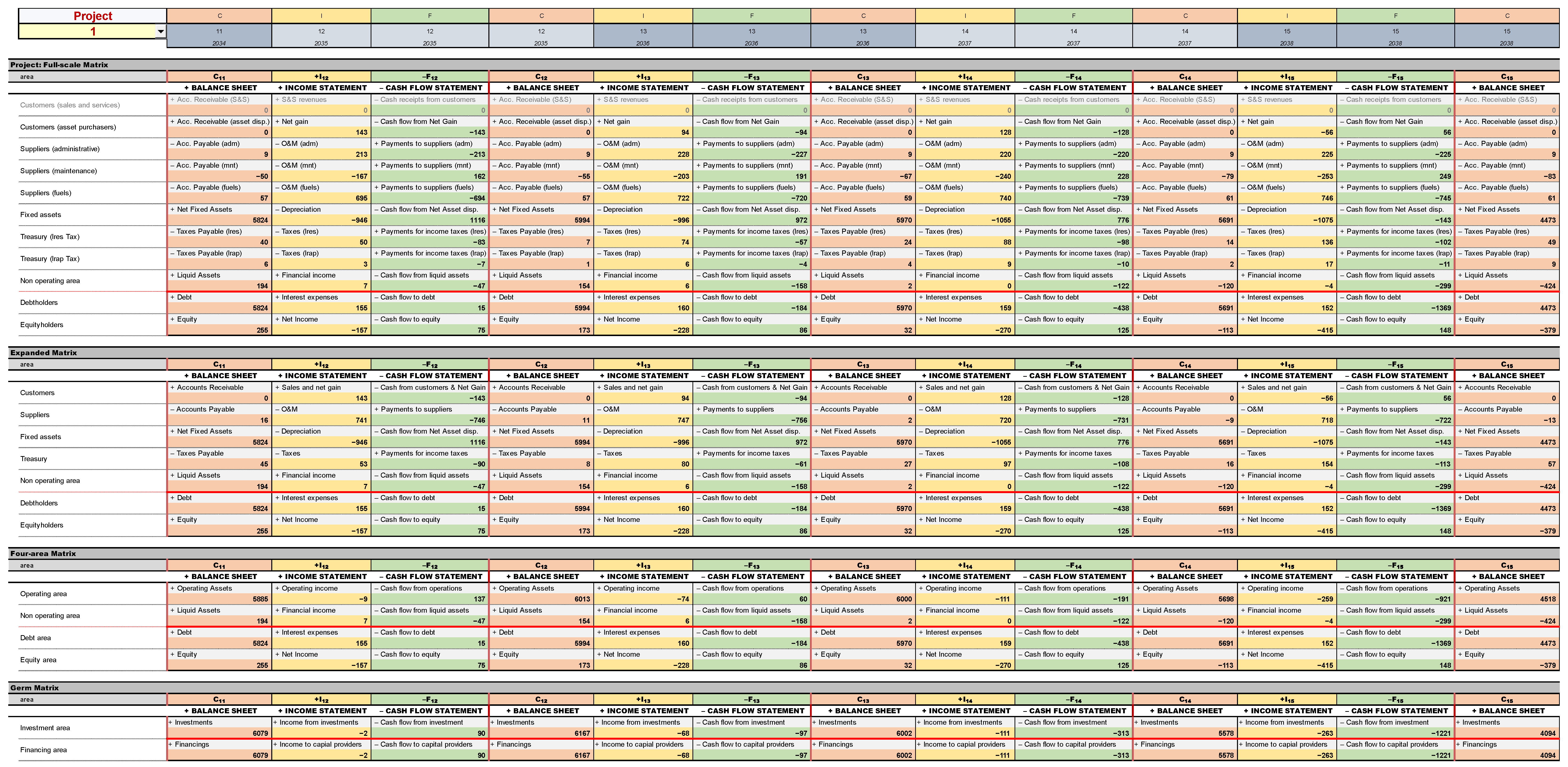
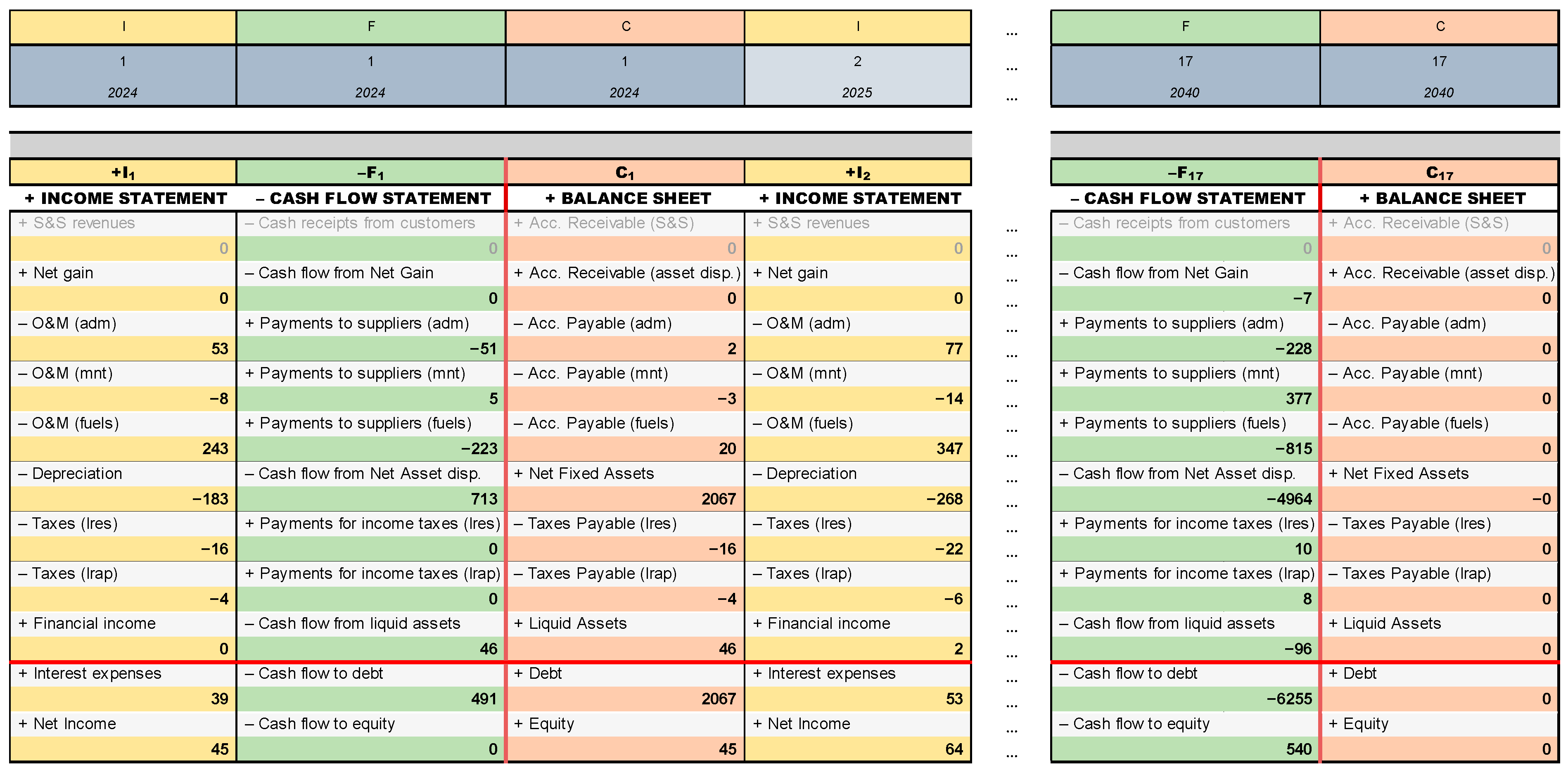
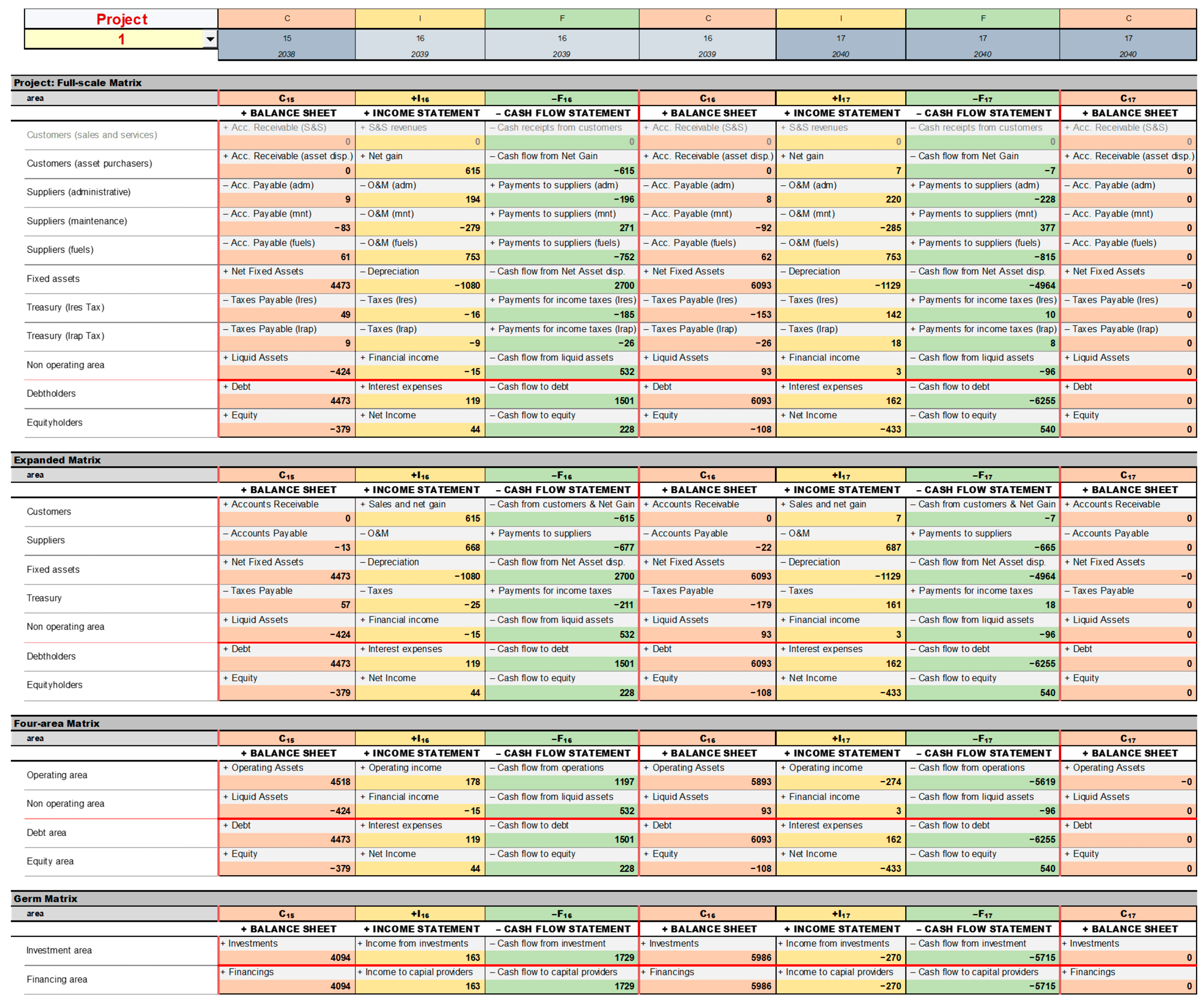
This framework leads to the creation of the so-called Split-Screen Matrix (SSM) for each year of the project’s lifespan and for every project. In our case, there is a sequence of SSMs, forming a comprehensive strip detailing the accounting and financial magnitudes of each project across every year. Figure 10 below reports an extract of the SSM strip for project 1 (see Figure A21, Figure A22, Figure A23, Figure A24 and Figure A25 for the whole SSM strip).

We do not dwell on the intricacies of this model and refer to the aforementioned contributions for the methodology and to Baschieri and Magni (2023) for spreadsheet modeling applications. In the latter, the authors show in detail how to apply the theoretical framework to spreadsheet modeling. In particular, the cells of this SSM strip can be divided into four groups.

Financial valuation. Once the SSM strip is built, we evaluate the model by using the Adjusted Present Value (APV) method (Myers, 1974), which presupposes the determination of the payout and financing policy and, hence, the determination of the interest tax shield.

The choice of the APV method over other common valuation methods, such as the FCF-WACC method (where free cash flows are discounted at the Weighted Average Cost of Capital), is motivated by the limitations of the latter, particularly its reliance on oversimplified financial planning. Specifically, payout and financing policies are not explicitly modeled, but are instead implicitly embedded in the assumption of a constant target leverage, which the firm is assumed to maintain through rebalancing, an assumption generally unrealistic in capital budgeting contexts: “The situation is which the firm’s capital structure is expected to change substantially over time, we recommend that the adjusted present value (APV) approach be used” (Titman & Martin, 2016, p. 333). In the same vein, Cooper and Nyborg (2007, p. 58) observe that “When valuing companies in transition or specific transactions or projects, one should generally assume that leverage will change over time—and the WACC approach should probably not be used. In such cases, the interest tax shields must be forecast year by year.”

Needless to say, the SSA is fully compatible with any valuation method, including both WACC- and APV-based approaches.

To manage risk, we rely on the Capital Asset Pricing Model (CAPM) to estimate the risk-adjusted costs of capital (Figure 11). For the cost of unlevered assets, we apply the formula

$$\stackrel{\mathrm{c}\mathrm{o}\mathrm{s}\mathrm{t} \mathrm{o}\mathrm{f} \mathrm{u}\mathrm{n}\mathrm{l}\mathrm{e}\mathrm{v}\mathrm{e}\mathrm{r}\mathrm{e}\mathrm{d} \mathrm{a}\mathrm{s}\mathrm{s}\mathrm{e}\mathrm{t}\mathrm{s}}{\overbrace{k^u}}=\stackrel{\mathrm{r}\mathrm{i}\mathrm{s}\mathrm{k}-\mathrm{f}\mathrm{r}\mathrm{e}\mathrm{e} \mathrm{r}\mathrm{a}\mathrm{t}\mathrm{e}}{\overbrace{r_f}}+\stackrel{\mathrm{u}\mathrm{n}\mathrm{l}\mathrm{e}\mathrm{v}\mathrm{e}\mathrm{r}\mathrm{e}\mathrm{d} \mathrm{b}\mathrm{e}\mathrm{t}\mathrm{a}}{\overbrace{{\beta }_u}}\cdot \stackrel{\mathrm{e}\mathrm{q}\mathrm{u}\mathrm{i}\mathrm{t}\mathrm{y} \mathrm{r}\mathrm{i}\mathrm{s}\mathrm{k} \mathrm{p}\mathrm{r}\mathrm{e}\mathrm{m}\mathrm{i}\mathrm{u}\mathrm{m}}{\overbrace{\left(r_m-r_f\right)}}.$$

We use the rate of return of 17-year government bonds as risk-free rate; for the unlevered beta, we use the data for the environmental-and-waste services sector reported in Damodaran’s “Betas by Sector” table (available at https://pages.stern.nyu.edu/~adamodar/New_Home_Page/datafile/Betas.html, accessed on 20 November 2023); for the equity risk premium in Italy, we use the data found in the Damodaran’s “Country Defaults Spreads and Risk Premiums” table (available at https://pages.stern.nyu.edu/~adamodar/New_Home_Page/datafile/ctryprem.html, accessed on 20 November 2023):

$$\stackrel{\mathrm{c}\mathrm{o}\mathrm{s}\mathrm{t} \mathrm{o}\mathrm{f} \mathrm{u}\mathrm{n}\mathrm{l}\mathrm{e}\mathrm{v}\mathrm{e}\mathrm{r}\mathrm{e}\mathrm{d} \mathrm{a}\mathrm{s}\mathrm{s}\mathrm{e}\mathrm{t}\mathrm{s}}{\overbrace{11.28\%}}=\stackrel{\mathrm{r}\mathrm{i}\mathrm{s}\mathrm{k}-\mathrm{f}\mathrm{r}\mathrm{e}\mathrm{e} \mathrm{r}\mathrm{a}\mathrm{t}\mathrm{e}}{\overbrace{4.12\%}}+\stackrel{\mathrm{u}\mathrm{n}\mathrm{l}\mathrm{e}\mathrm{v}\mathrm{e}\mathrm{r}\mathrm{e}\mathrm{d} \mathrm{b}\mathrm{e}\mathrm{t}\mathrm{a}}{\overbrace{0.86}}\cdot \stackrel{\mathrm{e}\mathrm{q}\mathrm{u}\mathrm{i}\mathrm{t}\mathrm{y} \mathrm{r}\mathrm{i}\mathrm{s}\mathrm{k} \mathrm{p}\mathrm{r}\mathrm{e}\mathrm{m}\mathrm{i}\mathrm{u}\mathrm{m}}{\overbrace{8.33\%}}.$$

We use the return of 17-year government bonds as a proxy for the return on non-operating assets as well because reinvestment in liquid assets will be essentially riskless: $r^l=4.12\%$. As for the required return on debt ($r^d$), we base our assessment on the average borrowing duration of 10 years. Consequently, we use the rate of return of 10-year government bonds as a proxy for the risk-free rate (assumed to be constant over subsequent years). The default spread is derived from Damodaran’s “Ratings, Interest Coverage Ratios and Default Spread” table (available at https://pages.stern.nyu.edu/~adamodar/New_Home_Page/datafile/ratings.html, accessed on 20 November 2023), reflecting the BBB rating recently issued by Standard & Poor’s.6 Hence,

$$r^d=\stackrel{\mathrm{r}\mathrm{i}\mathrm{s}\mathrm{k}-\mathrm{f}\mathrm{r}\mathrm{e}\mathrm{e} \mathrm{r}\mathrm{a}\mathrm{t}\mathrm{e} (10 \mathrm{y}\mathrm{e}\mathrm{a}\mathrm{r}\mathrm{s})}{\overbrace{3.88\%}}+\stackrel{\mathrm{d}\mathrm{e}\mathrm{f}\mathrm{a}\mathrm{u}\mathrm{l}\mathrm{t} \mathrm{s}\mathrm{p}\mathrm{r}\mathrm{e}\mathrm{a}\mathrm{d}}{\overbrace{2\%}}=5.88\%$$

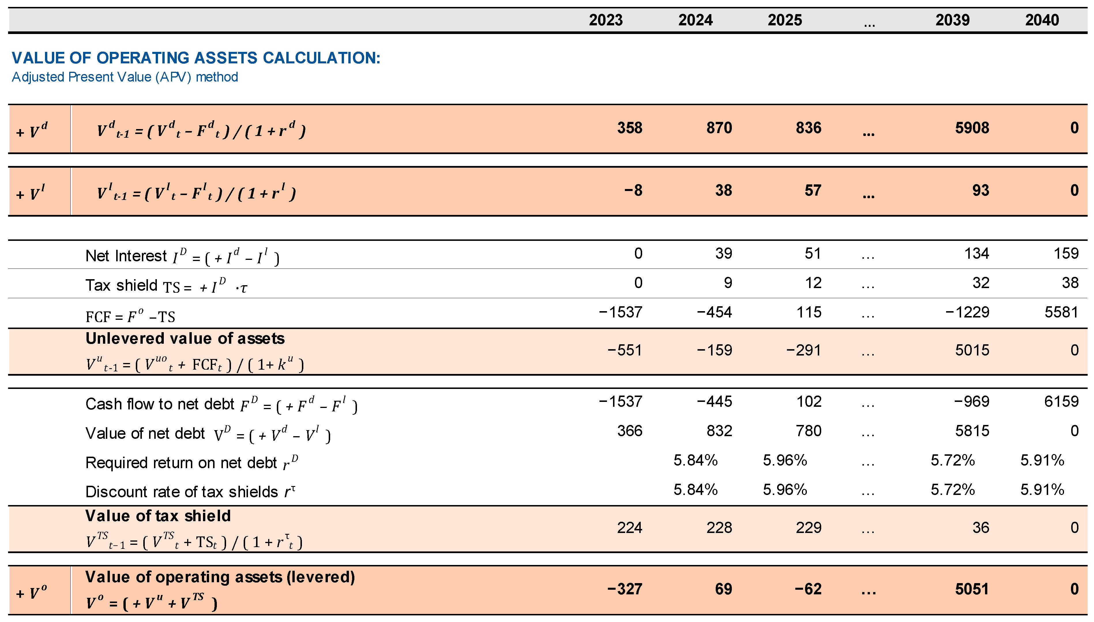
Lastly, we assume that the discount rate of tax shields equals the required return on net debt (i.e., debt net of liquid assets): $r^{\tau }=r^D$. The economic value of operating assets is then calculated as the sum of the unlevered value of assets and the value of tax shields, using backward induction:

$$V_t^o=\stackrel{\mathrm{u}\mathrm{n}\mathrm{l}\mathrm{e}\mathrm{v}\mathrm{e}\mathrm{r}\mathrm{e}\mathrm{d} \mathrm{v}\mathrm{a}\mathrm{l}\mathrm{u}\mathrm{e} \mathrm{o}\mathrm{f} \mathrm{a}\mathrm{s}\mathrm{s}\mathrm{e}\mathrm{t}\mathrm{s} V_t^u}{\overbrace{{\displaystyle \frac{V_{t+1}^u+{\mathrm{F}\mathrm{C}\mathrm{F}}_{t+1}}{1+k^u}}}}+\stackrel{\mathrm{v}\mathrm{a}\mathrm{l}\mathrm{u}\mathrm{e} \mathrm{o}\mathrm{f} \mathrm{t}\mathrm{a}\mathrm{x} \mathrm{s}\mathrm{h}\mathrm{i}\mathrm{e}\mathrm{l}\mathrm{d}\mathrm{s} V_t^{TS}}{\overbrace{{\displaystyle \frac{V_{t+1}^{TS}+{\mathrm{T}\mathrm{S}}_{t+1}}{1+r_{t+1}^{\tau }}}}}, t=\mathrm{0,1},\dots n-1, V_n^j=0$$

where ${\mathrm{F}\mathrm{C}\mathrm{F}}_t$ is the free cash flow, $r^{\tau }$ is the discount rate for tax shields, $\mathrm{T}\mathrm{S}$ is the Tax Shield ($=I_t^D·\tau )$, $\tau$ is the tax rate, and $I_t^D$ is the Interest expenses net of financial income ($I_t^d-I_t^l$). The market values of debt and non-operating assets are calculated in a backward fashion as well:

$$V_t^j={\displaystyle \frac{V_{t+1}^j+F_{t+1}^j}{1+r^j}}, t=\mathrm{0,1},\dots n-1, V_n^j=0$$

where $j=d,l$ (see Figure 12). Hence, the benchmark SSM is obtained, which makes use of the input market data. It displays the market values of the benchmark portfolios, together with their profits and cash flows. Value creation is calculated within the benchmark SSM. Specifically, we generate the differential SSM strip by subtracting each cell of the project SSM strip from its corresponding cell in the benchmark SSM strip. Within this strip, one can locate, for each year and business area (operating, non-operating, debt, and equity), the Market Value Added (MVA), the economic residual incomes (with changed signs), and the differential cash flows (see Figure A26 and Figure A27). We also calculate (i) the rates of return as the ratio of total profit to total invested capital (${\sum }_{t=0}^n{I}_t/{\sum }_{t=0}^n{C}_t$), (ii) the MARRs as the ratio of market-based profit to total invested capital (${\sum }_{t=0}^n{r}_t{V}_{t-1}/{\sum }_{t=0}^n{C}_t$) (see Magni, 2020),7 (iii) the financial efficiency (differences between rates of return and MARRs), and (iv) the scale (size) of each investment and financing area (Figure 13). The NPV is then reinterpreted as the product of the total capital committed and the financial efficiency:

$$\mathrm{N}\mathrm{P}\mathrm{V}=\mathrm{T}\mathrm{o}\mathrm{t}\mathrm{a}\mathrm{l} \mathrm{c}\mathrm{a}\mathrm{p}\mathrm{i}\mathrm{t}\mathrm{a}\mathrm{l}\times \stackrel{\mathrm{f}\mathrm{i}\mathrm{n}\mathrm{a}\mathrm{n}\mathrm{c}\mathrm{i}\mathrm{a}\mathrm{l} \mathrm{e}\mathrm{f}\mathrm{f}\mathrm{i}\mathrm{c}\mathrm{i}\mathrm{e}\mathrm{n}\mathrm{c}\mathrm{y}}{\overbrace{(\mathrm{r}\mathrm{a}\mathrm{t}\mathrm{e} \mathrm{o}\mathrm{f} \mathrm{r}\mathrm{e}\mathrm{t}\mathrm{u}\mathrm{r}\mathrm{n}-\mathrm{M}\mathrm{A}\mathrm{R}\mathrm{R})}}.$$

For example, Project 1, linked to scenario 1 (the green scenario characterized by the lowest degree of environmental compatibility), can be conceptualized as a portfolio consisting of two investments:

• an investment of 66.8 million euros in operating assets (net purchases of vehicles) with a financial (in)efficiency of $-$2.8%, resulting in an operating NPV of $-$€1.86 million
• an investment of €1.95 million in liquid assets (Iren Ambiente’s retained cash) with a financial (in)efficiency of $-$0.4%, resulting in a non-operating NPV of $-$€8 thousand.

Overall, the project’s NPV is negative and equal to $-$EUR 1,871,995 $=-$EUR 1,863,918$-$EUR 8077, that is, the undertaking of Project 1 will sacrifice about EUR 1.9 million of NPV as opposed to the status quo. However, due to Iren Ambiente’s favorable borrowing policy, the impact on economic value for the company’s shareholders is mitigated by the highly negative debt NPV of $-$EUR 1,179,564: the equity NPV is $-$EUR 692,431. The project NPV reflects the economic value captured by the capital providers, encompassing both equityholders and debtholders. However, the sole shareholder and debtholder of Iren Ambiente is the parent company, Iren Spa. Therefore, the project NPV represents the economic value acquired by Iren Spa. To sum up, the equity NPV delineates the value created for Iren Spa as a holder of Iren Ambiente’s shares, while the debt NPV delineates the value created for Iren Spa as a holder of Iren Ambiente’s debt. As all NPVs are negative, Iren Spa will inevitably face a financial burden regardless of the green policy adopted.

8. Outputs and Discussion

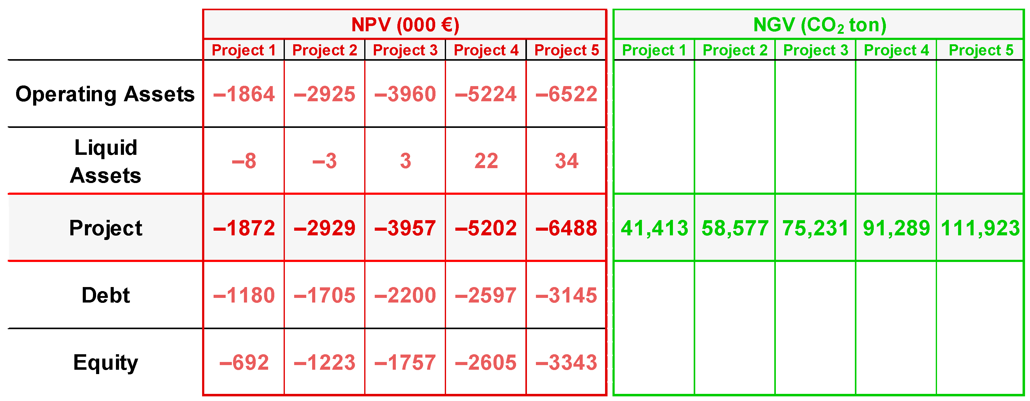
The outputs are divided into two classes: financial and environmental. The former comprises, for each business area and for each project, the total capital committed, the investment scale, the rate of return, the MARR, the financial efficiency, and the Net Present Value (NPV). 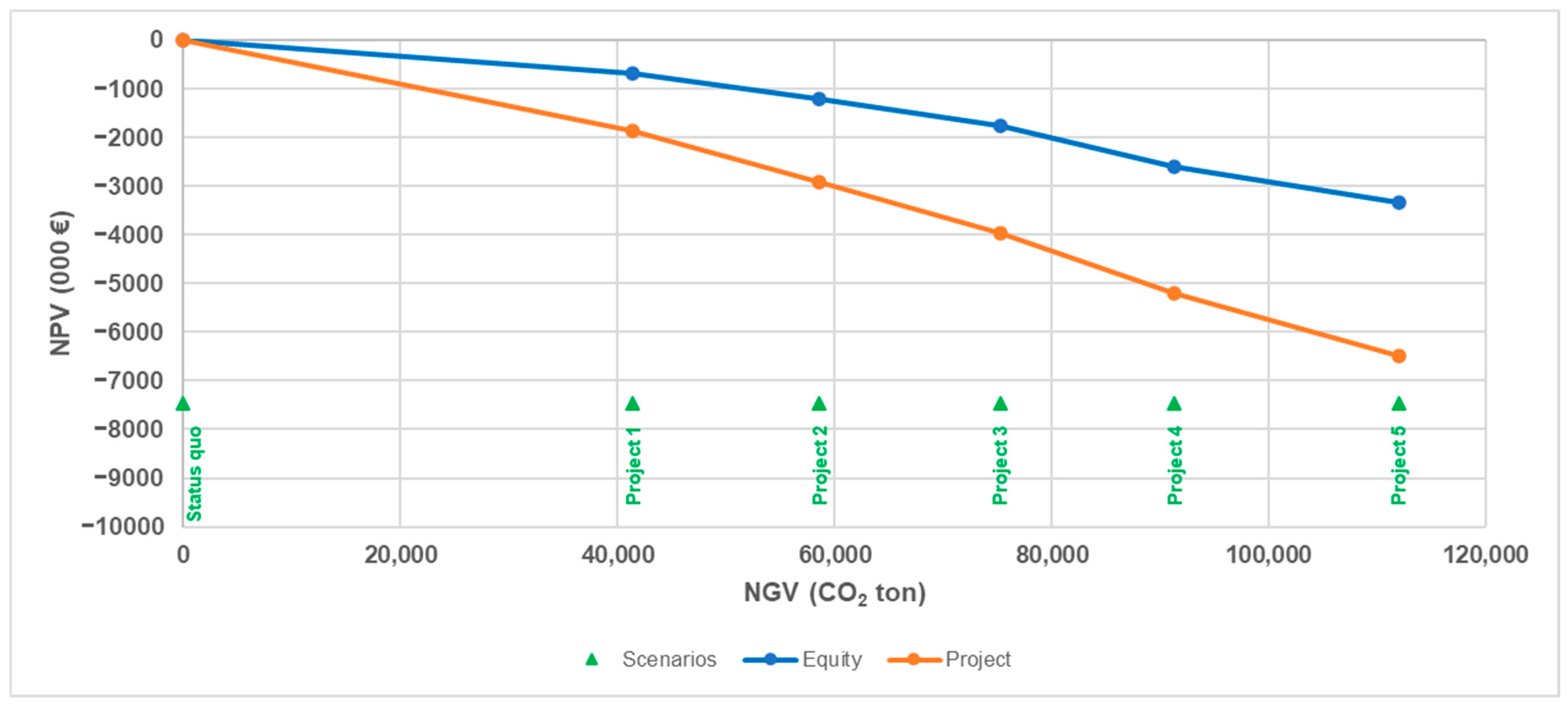The environmental output, directly derived from the Engineering Model, is given by the total CO₂ reduction, which we call the Net Green Value (NGV) (see Figure 14). We plot the five combinations of NGV and NPV on an $xy$-plane, resulting in the Net Value curve (see Figure 15). This curve associates the NGV (horizontal axis) with the NPV (vertical axis). Each scenario generates a project, and each project gives rise to a point on the curve, illustrating the project NPV and the project NGV (we report both the project NPV and the equity NPV). We note that, as the NGV increases, both the project NPV and the equity NPV decrease, indicating a decreasing relationship between economic value and environmental value: the pursuit of environmental gain results in a financial setback. Also, note that the NPV of each scenario is negative. More precisely, focusing on project NPVs (values in thousands of euros), the NPV of Project 1 is $-$1872, the NPV of Project 2 is $-$2929, the NPV of Project 3 is $-$3957, the NPV of Project 4 is $-$5202, the NPV of Project 5 is $-$6488. Therefore, progressively higher amounts of financial value are sacrificed. In contrast, environmental value is created (in terms of CO₂ ton reduction) for every scenario and, in particular, the NGV of Project 1 is 41,413, the NGV of Project 2 is 58,577, the NGV of Project 3 is 75,231, the NGV of Project 4 is 91,289, the NGV of Project 5 is 111,923. Therefore, there is a trade-off between “being greener” and “being richer”: the objective of maximizing the NGV would lead the company to select the challenging scenario 5, whereas the objective of maximizing the NPV would lead the company to select the status quo, representing no change in the current replacement policy. The piece of information provided by the Net Value curve is significant as it quantifies the value the company must give up in exchange for an increase in the degree of its environmental sustainability. In other words: the Net Value curve reveals the “cost of being greener”. The ratio of the (absolute value of) NPV to the NGV supplies an average rate of substitution, that is, the “shadow” price for one metric ton of CO₂ reduction with respect to the status quo. Specifically, from the point of view of Iren Spa, the “shadow” price for Project 1 is 45.20 EUR/ton CO₂, the “shadow” price for Project 2 is 50.00 EUR/ton CO₂, the “shadow” price for Project 3 is 52.60 EUR/ton CO₂, the “shadow” price for Project 4 is 56.98 EUR/ton CO₂, the “shadow” price for Project 5 is 57.97 EUR/ton CO₂, (Figure 16). These shadow prices are measured in units of NPV. They indicate the NPV sacrificed by Iren Ambiente when undertaking Project s $=$ 1, 2, 3, 4, 5 for a unit reduction in CO₂. 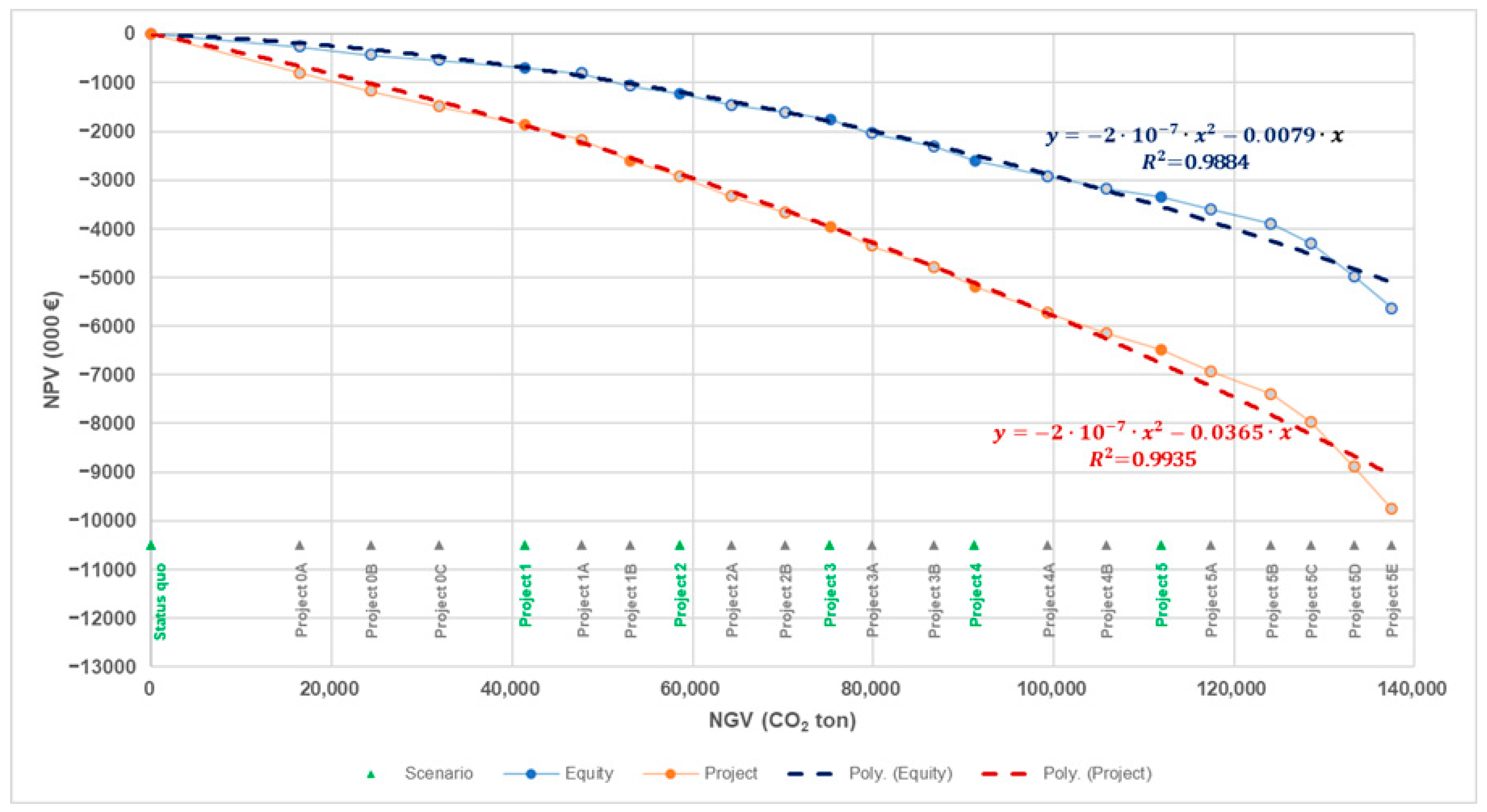For example, if Iren Ambiente chooses green policy 3, Iren Spa will “pay” EUR 52.60 (in NPV units) per ton of CO₂ for increasing the sustainability of Iren Ambiente’s operating assets by 75,231 tons from 2024 to 2040 compared with the current replacement policy. To further investigate the functional relation between the NGV and NPV, we extend the analysis to additional 16 green scenarios. Overall, we consider 21 green scenarios, from a scenario with no reduction in CO₂ (status quo, scenario 0) to a scenario with nearly 140,000 tons of CO₂ reduction. We plot the NGV-NPV pairs and connect the points. The result is a strictly decreasing and generally concave function of NGV (Figure 17).8 The (slight) concavity is verified by a degree-2 polynomial regression; for example, the polynomial $y=-2\cdot {10}^{-7}\cdot x^2-0.0079\cdot x$ fits the equity Net Value curve very well with its high determination coefficient: R² = 0.9884 (see Figure 17). Analogously with the project Net Value curve, which shows an even higher determination coefficient, equal to R² = 0.9935. The general concavity of the functions implies that the marginal rate of substitution is generally increasing. In other words, as one moves along the curve and increase CO₂ reduction, the sacrifice in terms of NPV becomes progressively greater.9

Given that Iren Ambiente aims at optimizing both objectives, its managers had to select, based on strategic considerations, the preferred solution. IREN places great importance on both the economic sustainability and the profitability of its shareholders (both public and private), but equally important is its concern for the environment and the territories in which it operates. IREN’s Action Plan to 2030, outlining its medium- and long-term trajectory, is in line with ecological transition principles, emphasizing the centrality of communities and individuals. The plan is structured around five key focus areas: decarbonization, circular economy, water resources, resilient cities, and people. This strategic vision is underpinned by a reinforced investment plan, totaling 10.5 billion euros over 8 years). Approximately 7.5 billion euros, constituting 80% of the organic investments, is allocated to projects aligned with the established sustainability goals. This initiative notably bolsters city resilience and drive decarbonization efforts. IREN is evaluated by various ESG rating agencies, and its ESG rating reflects strong performance (e.g., CDP Climate Change awards A-level, MSCI rates A out of a maximum of AAA), and the Group hopes to consolidate or improve it. For these reasons, maintaining the status quo about waste vehicle replacement policies could not be an option in the IREN Group’s plans.

After learning about the trade-off between economic and environmental benefits and considering that the greenest scenarios imply negative NPVs of many millions of euros, Iren Ambiente has opted for Scenario 2, a greener policy than the status quo, but one that remains cautious or balanced.

While Figure 16 confirms that Project 1 (Scenario 1) offers the lowest CO₂ shadow price (EUR 45.20/ton), the choice of Scenario 2 reflects management’s holistic evaluation of three main factors:

• strategic trade-offs: Scenario 2’s higher CO₂ reduction (58.6k vs. 41.4k tons) justified its greater NPV sacrifice (−EUR 1223M vs. −EUR 692M equity NPV) and is in alignment with IREN Group’s decarbonization targets,
• operational feasibility: a sudden shift to aggressive electrification (e.g., Scenario 5) would put pressure on maintenance personnel skilled in diesel engines, logistics (recharging cycles), and supplier capacity (bulk-order delays),
• risk mitigation: geopolitical and socio-economic instability favors risk-averse transitions, while IREN’s EUR 10.5 billion Action Plan prioritizes gradual decarbonization.

More cautious scenarios (Scenario 1) would undermine sustainability targets; more green-aggressive scenarios (Scenarios 3–5) jeopardize essential waste management operations during the period of workforce and supplier adaptation. According to IREN’s management, shadow prices do inform, but cannot override such multidimensional judgments, especially given that operational departments may struggle to support a total or near-total conversion from vehicles with traditional fuels to electric or natural gas. While these options are compatible with the service, they demand cultural adaptation by operational workers and managerial adaptation by coordinators, who, for example, will have to gradually organize vehicle rotations to allow complete electric recharge cycles. Even corporate maintenance garages, whose mechanics currently specialize in diesel engines (which are prevalent today), will have to train their personnel and equip their facilities to service alternative-fuel vehicles, with a gradual transition. Finally, vehicle suppliers themselves are progressively expanding their production of green vehicles, enhancing their reliability over time. However, extended delivery times are common, especially for “bulk” orders. A balanced green policy will ensure better alignment with the procurement capabilities of IREN’s domestic partner suppliers.

It is common practice at IREN to pursue Green Mobility initiatives (see Section 3), even when this implies a partial sacrifice of short-term economic value in favor of long-term sustainability benefits. In the specific case analyzed, IREN’s management, who have oversight of all group-wide green projects, including those outside of waste management, identified Scenario 2 as the preferred option. Their choice was based on its optimal balance between economic impact and environmental benefit, in line with IREN’s broader decarbonization strategy.

Thus, Scenario 2 emerged as optimal equilibrium between financial viability, environmental impact, and implementation feasibility. While shadow prices did not override this specific decision, they remain an essential tool for future capital budgeting, enabling firms to quantify sustainability trade-offs in financial terms. As stakeholder pressure for transparent environmental accounting rises, shadow pricing may evolve from analytical novelty to operational necessity.

The two-dimensional scenario-analysis matrix in Figure 18 plots Net Green Value (NGV) against Net Present Value (NPV) to evaluate and categorize projects based on both financial return (NPV) and environmental impact (NGV). The vertical axis represents NPV, which measures the economic value created: projects above the horizontal axis are economically profitable, while those below cost more than they return. The horizontal axis represents NGV, which measures environmental benefit in terms of CO₂ emissions reduced: projects on the right have positive NGV and contribute to climate goals, while those on the left have negative NGV and increase emissions. The matrix is divided into four quadrants:

• Top right—“Win-Win” projects: positive NPV and positive NGV, both profitable and climate-positive.
• Top left—“Profit-Driven” projects: positive NPV but negative NGV, financially attractive yet environmentally harmful.
• Bottom left—“Lose-Lose” projects: negative NPV and negative NGV, economically unprofitable and environmentally damaging (to be avoided or phased out).
• Bottom right—“Sustainability-Driven” projects: negative NPV but positive NGV, environmentally beneficial but not financially viable.

The analysis of the 21 scenarios and the resulting Net Value Curve provides a clear, empirical basis for managerial decision-making. The curve serves as a strategic map, quantifying the financial sacrifice required for each additional unit of environmental benefit. To operationalize this tool, managers can follow a structured, three-step guide:

• Identify the Efficient Frontier: The Net Value Curve itself represents the set of Pareto-efficient projects. Any point on this curve is a candidate for selection, while points below represent inefficient strategies.
• Define the Shadow Price Threshold: Determine the maximum financial sacrifice (in NPV) per metric ton of CO₂ reduced that the organization is willing to bear. This internal shadow price can be derived from the curve itself (as in Figure 16) and calibrated against the company’s strategic sustainability targets and financial constraints.
• Select the Optimal Project: Identify the point on the curve where the trade-off between NPV and NGV aligns with the strategic priorities defined in Step 2. This selects the projects that deliver the highest possible environmental benefit without exceeding the acceptable cost per ton of CO₂.

This structured guide allows decision-makers to move directly from the visual representation of the trade-off to a concrete project selection.

It is important to distinguish the shadow price introduced in this study from market-based carbon prices (e.g., the EU Emissions Trading System—EU ETS). Our shadow price is an internal financial indicator that measures the sacrifice in shareholder value (NPV) required to avoid one ton of CO₂ emissions. In contrast, an external carbon price represents the cost imposed by the market or a regulator for the right to emit one ton of CO₂. An external carbon price is a potential model input: if a company is subject to a carbon tax or must purchase emission allowances, this cost is directly incorporated into the project’s financial statements (e.g., as an additional operating cost). This incorporation alters the project’s cash flows and its NPV, thereby changing the position and shape of the Net Value Curve and the resulting internal shadow price. In this framework, the shadow price is the definitive output metric that synthesizes the total financial impact of the green transition, inclusive of all regulatory costs. The managerial decision involves judging whether to internalize an expected future carbon price into the model. A carbon price exerts two opposing forces on green investments: a negative effect that reduces all projects’ NPVs by increasing energy costs, and a positive effect that progressively favors greener scenarios by proportionally reducing their carbon tax burden. The net effect is therefore an empirical question that depends on the specific carbon price level and the fleet’s emission profile.

9. Sensitivity Analysis

We model risk through the quantification of systematic risk via CAPM, which incorporates it into discount rates. The model captures this risk using the unlevered beta, reflecting exposure to macroeconomic shocks affecting the environmental services sector. By anchoring valuations to unlevered betas, we ensure that systematic risks beyond IREN’s control are properly accounted for, thus preventing potential mispricing.

Another important tool for managing risk is sensitivity analysis on the main market input parameters. In this section, we perform scenario analysis on key inputs such as financial market data and energy prices, to evaluate the impact of fluctuations on the NPV. Future research may refine risk analysis by adopting more advanced methods, such as the Clean Finite Change Sensitivity Index (Magni et al., 2020), a novel technique for quantifying the effect of individual value drivers on NPV and other financial metrics.

We begin with a sensitivity analysis of the main financial market input data: the unlevered beta ($\beta$), the equity risk premium, and the default spread. For our case study, the estimated values are $\beta =0.86$, Equity Risk Premium $=8.33\%$, and default spread $=2\%$. We refer to these values as the base case and analyze the impact on the NPV of both upward and downward deviations from those values. Specifically, we consider the following scenarios:

• perturbation of $\beta$ (from 0.7 to 1), with other market inputs held constant,
• perturbation of Equity Risk Premium (from 4% to 12%), with other market inputs held constant,
• perturbation of spread (from 1% to 3%), with other market inputs held constant
• simultaneous perturbation of $\beta$, Equity Risk Premium, and default spread: from (0.7, 4%, 1%) to (1.0, 12%, 3%).

The results, presented in

Table 2. Sensitivity analysis for market input data.

		Net Present Value (Project)
Beta (β)		Status quo	Project 1	Project 2	Project 3	Project 4	Project 5
Downside case	=0.70	0	−1798	−2843	−3824	−5120	−6424
Base case	=0.86	0	−1872	−2929	−3957	−5202	−6488
Upside case	=1.00	0	−1917	−2977	−4036	−5237	−6502
Equity Risk Premium		Status quo	Project 1	Project 2	Project 3	Project 4	Project 5
Downside case	=4.00%	0	−1581	−2571	−3426	−4815	−6125
Base case	=8.33%	0	−1872	−2929	−3957	−5202	−6488
Upside case	=12.00%	0	−1961	−3017	−4111	−5240	−6463
Default spread		Status quo	Project 1	Project 2	Project 3	Project 4	Project 5
Downside case	=1%	0	−1848	−2894	−3913	−5148	−6420
Base case	=2%	0	−1872	−2929	−3957	−5202	−6488
Upside case	=3%	0	−1894	−2960	−3997	−5110	−6547
Beta/Equity Risk Premium/Default spread		Status quo	Project 1	Project 2	Project 3	Project 4	Project 5
Downside case	=(0.70, 4.00%, 1%)	0	−1474	−2429	−3229	−4632	−5922
Base case	=(0.86, 8.33%, 2%)	0	−1872	−2929	−3957	−5202	−6488
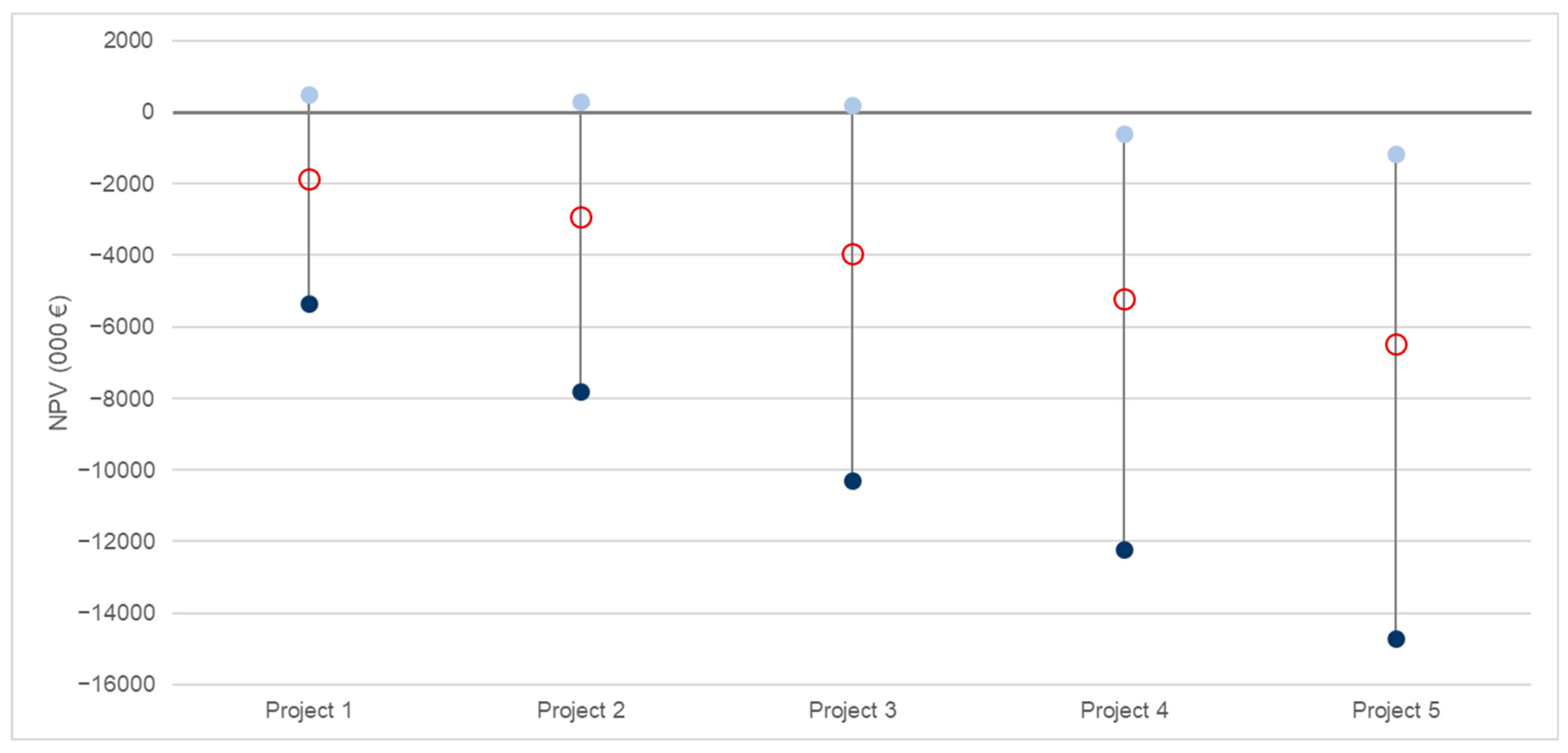
Upside case	=(1.00, 12.00%, 3%)	0	−1999	−3054	−4172	−5112	−6448

, indicate that variations in market input data do not alter the relationship between NPV and NGV: in all cases, the NPV decreases as the scenario index increases. Also, the absolute variation in NPV resulting from the perturbations is relatively limited. This behavior can be visually observed in Figure 19, which illustrates the results of the last case, where three market inputs are simultaneously perturbed.

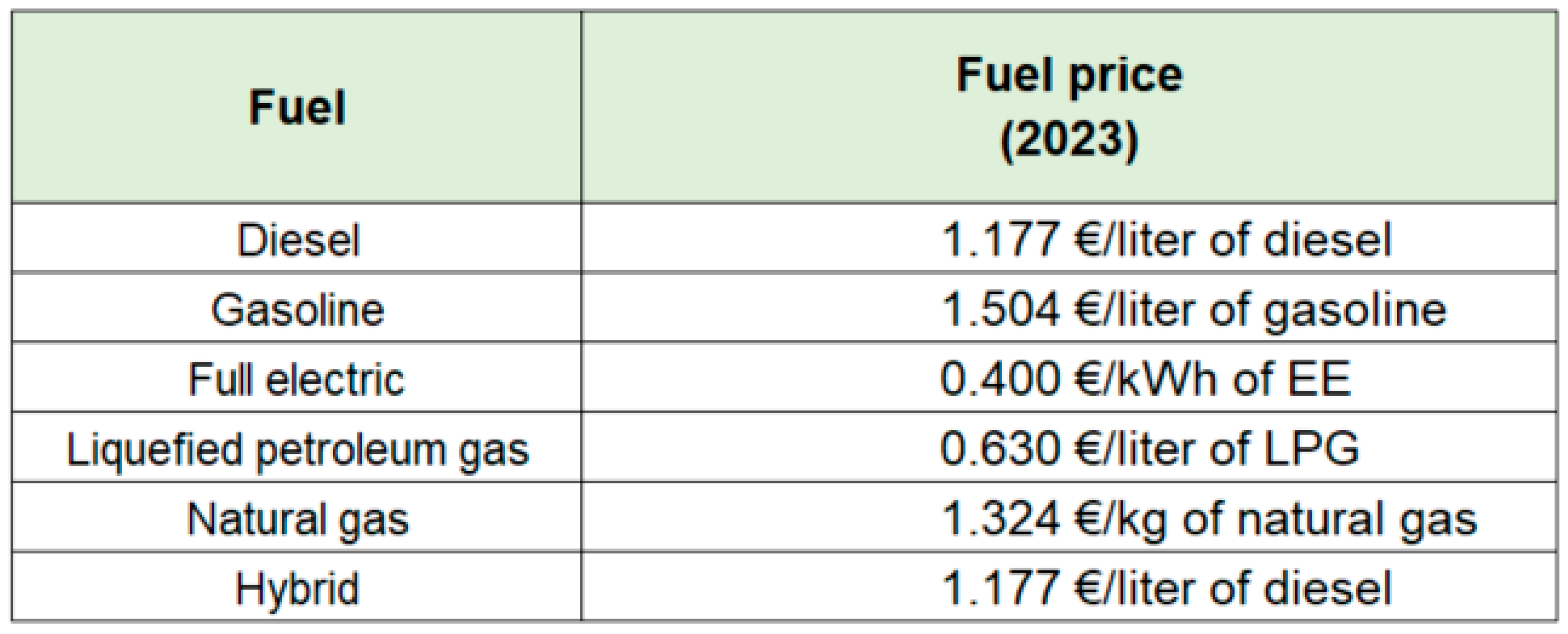
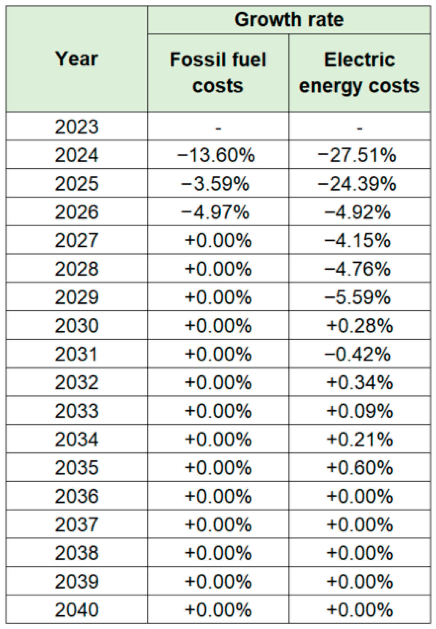
An important variable affecting the NPV is the cost of the fuels by the fleet (primarily diesel in Scenario 0, primarily electricity in Scenario 5). We now examine the sensitivity of the NPV to changes in fuel prices. Figure 20 and Figure 21 report, respectively, the fuel prices in 2023 and their projected annual growth rates, as provided by IREN. Unit fuel costs for the period 2024–2040 are calculated by applying the corresponding respective growth rates to the 2023 baseline values.

As can be gleaned from Figure 21, IREN estimates a decrease in the fossil fuel costs between 2023 and 2026, followed by stable prices thereafter. The average decrease is $-1.3\%$. Regarding electricity costs, IREN forecasts a decrease from 2023 to 2030, after which the prices are expected to remain essentially stable. The average decrease is $-4.13\%$. We also note that

• the average change in diesel prices in Italy from 2004 to 2023 has been $+4.04\%$
• the average change in electric energy price (PUN) in Italy over the same period has been $+16\%$.10

Based on this, we choose to perturb the average decrease estimated by IREN by selecting an interval whose lower bound corresponds to the historical averages mentioned above, and whose upper bound is symmetrically set with respect to the base case (see Figure 22).

The base case assumes that both fossil fuel and electric energy will decrease over time. If, instead, the fossil fuels grew (by an average $4.04\%$ per year), all other things equal, each scenario yielded a net financial benefit to IREN. Indeed, Projects 1 and 2 would even become positive-NPV alternatives. Conversely, if the electricity price (rather than fossil fuel price) were to increase (by an average $16\%$ per year), the transition toward environmentally friendly procurement policies would become less favorable compared with the base case (see

Table 3. Sensitivity analysis on fuel costs.

		Net Present Value (Project)
Price growth of fossil fuel cost		Status quo	Project 1	Project 2	Project 3	Project 4	Project 5
Downside case	=−6.64%/y	0	−2573	−3895	−5201	−6589	−8095
Base case		0	−1872	−2929	−3957	−5202	−6488
Upside case	=+4.04%/y	0	282	17	−177	−1010	−1651
Price growth of electric energy cost		Status quo	Project 1	Project 2	Project 3	Project 4	Project 5
Downside case	=−24%/y	0	−1660	−2632	−3570	−4775	−5987
Base case		0	−1872	−2929	−3957	−5202	−6488
Upside case	=+16%/y	0	−4652	−6825	−9057	−10,829	−13,094
Price growth of both fuel costs (fossil and electric energy)		Status quo	Project 1	Project 2	Project 3	Project 4	Project 5
Best case	(+4.04%, −24%)	0	494	314	212	−582	−1149
Base case		0	−1872	−2929	−3957	−5202	−6488
Worst case	(−6.64%, +16%)	0	−5352	−7791	−10,301	−12,218	−14,707

). By combining the two favorable cases (fossil fuel costs rising by $4.04\%$ and electricity prices falling by $24\%$) or the two unfavorable ones (fossil fuel prices falling by $6.64\%$ and electricity prices rising by $16\%$), we obtain, respectively, the best and worst outcomes (see the final panel of Table 3 and Figure 23).

10. Concluding Remarks

This paper deals with financial decision-making regarding vehicle replacement projects. From an engineering perspective, the focus is on the technical features, optimization processes, and the selection of the most appropriate optimization tool. In contrast, in finance, capital budgeting projects are analyzed through pro forma financial statements, estimating book values, revenues, costs, earnings, and appraised using some financial metric (e.g., NPV, rates of return, residual income). This paper aims to integrate the two perspectives by developing an accounting-and-finance system in which an engineering model processes a large number of technical inputs and feeds a comprehensive financial model, which carries out both financial planning and financial valuation for the projects under consideration.

We analyze the case of Iren Ambiente, a subsidiary of IREN Group, which needs to define a strategic vehicle replacement plan in accordance with IREN Group’s Action plan toward “green” mobility. We find a trade-off between “being greener” and “being richer”: the main output of the overall modeling is a Pareto frontier, called Net Value curve, showing the combination of Net Present Value (measuring the value creation) and Net Green Value (measuring the reduction in CO₂ emissions). In practice, it quantifies how much value the company must give up to increase the degree of its environmental sustainability, and it is an effective tool that may support Iren Ambiente’s managers in their decision, according to strategic considerations. The work performed, in addition to providing IREN with a much more advanced and comprehensive decision-support tool than is currently available in the company for analysis on this planning issue, attests that, unfortunately, nowadays and in the medium-term forecasts, choosing green fuels to reduce emissions may involve higher overall costs for the company, resulting in value destruction. We evaluated a large number of scenarios and also estimated the shadow price for IREN, expressing the cost of each ton of CO₂ reduction.

Our research question was how a capital-budgeting framework can integrate extensive operational and financial inputs into a dynamically consistent model that preserves accounting–valuation coherence, incorporates financing and distribution policies, and reconciles pro forma statements with valuation metrics. The application shows that the Split-Screen Approach effectively addresses this challenge, providing IREN managers with consistent, transparent decision support.

While the study has been conducted in the specific context of IREN’s heterogeneous waste-collection fleet, the approach is not restricted to this case. The framework is generalizable to other fleets, utilities, and large-scale infrastructure projects that require rigorous integration of engineering inputs with accounting and financial planning. This transferability makes the Split-Screen Approach a scalable tool for complex capital budgeting decisions beyond the waste-management sector.

While our model enables integrated technical-economic appraisal of vehicle replacement, several of its assumptions present opportunities for extension. For example, green policy modeling could be made more dynamic by allowing fuel selection policy for each vehicle type to be adjusted multiple times over the planning horizon. Likewise, the model could be enhanced to account for changes in the total number of vehicles per type over time (currently, the model restricts attention on inertial investments, assuming that the number of vehicles per type and in total remains constant, with only fuel composition varying). Additional flexibility could be introduced by incorporating exceptions to the maximum age limit for certain vehicles under specific conditions. Moreover, expanding the model to include broader environmental indicators could help generate more targeted sustainability recommendations. While our analysis focuses on CO₂ reduction as an internal metric of environmental performance, future research could extend the framework by considering EU-carbon prices, providing additional insight into the economic significance of environmental impacts and supporting decision-making where carbon pricing is relevant. Specifically, the framework opens the way to analyzing the interaction between internal financial trade-offs and external regulatory pressures. An insightful extension would be to incorporate an explicit carbon price (e.g., mirroring the EU ETS) as a key model input. This would dynamically reshape the Net Value Curve. However, the net effect, resulting from a trade-off between increased operational costs and the relative financial advantage of a reduced compliance burden for lower emissions, cannot be determined a priori. Quantifying this effect and identifying the carbon price threshold at which the green transition becomes NPV-positive would provide critical insights for strategic planning under evolving regulatory scenarios.

Further refinements are possible through operations research techniques: rather than treating green purchasing percentages as fixed scenario inputs, one could model them as decision variables within a constrained bi-objective optimization framework, aiming to maximize both NPV and NGV. In this context, integer programming formulations, extending classical equipment replacement models, offer a promising avenue for integrating financial and environmental goals.

Although our CAPM-based analysis provides a foundation for assessing risk, the high number of inputs parameters naturally raises questions about how to quantify their effects on key outputs. To enhance the understanding of risk exposure, a stochastic modeling approach could be adopted, where key accounting and financial figures are treated as random variables. This could be implemented through techniques like Monte Carlo simulation to propagate uncertainty through the model. However, our preliminary sensitivity analysis suggests that changes in market input data do not significantly affect either the NPV or its relationship with NGV. This relationship holds even when variations in energy prices are considered. We acknowledge that a fully comprehensive sensitivity analysis presents significant complexity, as our framework does not evaluate a single project but multiple projects associated with different environmental policies. This multi-scenario context calls for a multidimensional sensitivity analysis, which would require substantial computational effort and a dedicated methodological exposition. These scope conditions should not be read as weaknesses but as natural boundaries of our contribution, which is purposefully focused on financial planning and financial evaluation within an accounting-and-finance perspective. In this regard, a promising future direction involves applying more comprehensive approaches such as the Clean Finite Change Sensitivity Index (Magni et al., 2020), which could precisely quantify each input’s contribution to value creation across alternative policy scenarios.

The Net Value curve and shadow prices provide IREN managers with practical guidance for vehicle replacement decisions, highlighting the trade-off between financial value and CO₂ reduction. This framework allows prioritization of investments that maximize sustainability within acceptable financial costs, while the Split-Screen Approach ensures consistency with accounting, planning, and valuation principles.