Abstract
The increasing complexity of energy systems amid the global push for decarbonization raises important questions about how transitions in the energy matrix affect financial risk in electricity markets. This study investigates the relationship between structural changes in national energy matrices and the systemic risk associated with electricity prices in Europe from 2015 to 2022. Using daily electricity price data, we calculate log returns and estimate the Value at Risk (VaR) at the 1% level as a measure of extreme financial loss. We incorporate energy market variables, including the volatility of Brent oil and coal prices, and an entropy-based indicator derived from the Shannon index, which captures the degree of technological dispersion in the energy mix over time. A fixed-effects panel regression model is applied across 21 European countries to identify the drivers of energy-related financial risk. Results show that higher volatility in Brent and coal prices significantly increases the VaR, and that greater entropy reflecting a more complex and dynamic energy transition also correlates with higher systemic risk. These findings suggest that while energy diversification is a goal of sustainability, it may entail short-term instability. The study contributes to the understanding of how structural transformations in energy systems interact with financial vulnerabilities in liberalized electricity markets.
1. Introduction
Energy is a fundamental component of the economy, encompassing diverse sectors such as production, distribution, and consumption. It is recognized as the engine of economic growth and an essential element for the progress of society (Y. Qin & Zhang, 2024). In this context, the transition towards more diversified and sustainable energy matrices poses new challenges in terms of financial stability, especially in liberalized electricity markets. This study explores how the composition and evolution of the energy matrix impact the financial risk associated with electricity prices, highlighting the role of the energy transition as a possible amplifying factor of volatility.
Despite the consensus on the need to move toward cleaner and more diverse energy systems, little research has been carried out on how these structural transformations affect the financial behavior of electricity markets. The incorporation of intermittent sources such as wind or solar, along with the reduction in conventional sources, can generate additional tensions in the system, affecting price predictability and amplifying risk exposure. Dincer and Abu-Rayash (2020) define an energy system as the set of processes through which energy is transformed and distributed from primary sources to end users, delivering services such as electricity, heating, cooling, and hot water. Similarly, Chen et al. (2014) conceptualize the energy structure in terms of the origin of energy generation and the composition of the energy mix. Furthermore, technological changes are not homogeneous across countries, which introduces heterogeneity into energy transition trajectories. In this scenario, it is crucial to identify whether greater energy diversity, valued as positive from an environmental perspective, could also be associated with higher levels of financial risk in the short term. This ambiguity creates a significant gap in the literature and raises questions for policymakers and market participants. Energy diversification operates as a financial risk mitigation mechanism closely aligned with the principles of Modern Portfolio Theory (Markowitz, 1952). By distributing exposure across different energy sources and technologies, it reduces the vulnerability of supply and revenues to geopolitical shocks, natural disasters, and environmental disruptions, while helping stabilize prices (Cooray et al., 2025). In this study, we hypothesize that increasing the diversification of the energy matrix, measured through the composition of generation sources and the Shannon entropy of technological transitions, reduces financial risk in electricity markets, as reflected in Value at Risk (VaR) of electricity prices. Following the logic of portfolio diversification, distributing energy supply across multiple sources mitigates vulnerability to price shocks, supply interruptions, and generation failures, thereby enhancing market stability and resilience. Beyond energy markets, diversification is supported by financial development and technological progress, which enable clean energy investment and drive sustainable economic growth, although the speed of transition varies across countries (Nguyen et al., 2025). At the project level, diversification within renewable infrastructures for instance, spreading generation across multiple wind turbines lowers the impact of individual failures and significantly reduces tail-risk measures, thereby reinforcing financial resilience (Mikindani et al., 2025).
To measure financial risk, we use Value at Risk (VaR) (X. Wang et al., 2024), complemented with entropy measures and Markov chains to capture how energy mix complexity influences electricity market volatility. Previous research has examined volatility, contagion, and diversification in energy markets. For instance, Jude et al. (2023) analyze volatility and spillover effects between energy and stock markets in Central and Eastern Europe during major crises, finding that oil-related shocks exert the strongest contagion effects. Janczura and Puć (2023), propose short-term diversification strategies to minimize price risk in wholesale electricity markets, highlighting the importance of volatility forecasting for operational planning. Božičević Vrhovčak and Malbašić (2023) focus on the evolving role of aggregators in European electricity markets, emphasizing regulatory challenges and price dynamics that affect demand response integration, while Londoño and Velásquez (2023) provide an overview of research trends in electricity market risk management. Ewald et al. (2024) explore how physical climate risks impact traditional and renewable energy markets in China, revealing differentiated effects on energy commodities. Unlike these studies, our work centers on technological transitions within the energy mix as potential amplifiers of systemic risk, offering a novel empirical contribution to understanding volatility in the context of the energy transition and liberalized electricity markets.
The analysis is performed using daily time series of energy prices. From these prices, returns are calculated to estimate VaR, using data downloaded from Bloomberg and ENTOS-E. The energy matrix is structured based on annual production data for different generation types (Ritchie & Rosado, 2020). To address this question, we employ a panel data regression model with fixed effects, which allows us to analyze how different energy sources affect risk under different market conditions. This approach ranges from the most extreme losses (1st percentile) to the least severe, assessing the average effect, including the composition of the energy mix, which influences risk depending on the level of market stress.
The analysis of transitions between major energy production sources, such as nuclear, coal, wind, oil, gas, and hydropower, is performed using Markov chains, which allow for the identification of patterns of change in the energy matrix and the assessment of their impact on market volatility. This approach is novel and particularly relevant in the context of the energy transition, as it offers insight into how fluctuations in the production matrix, derived from variations in these energy sources, affect the stability and risk of energy markets. The Shannon index is incorporated into this framework as an entropy measure that captures the degree of complexity and dynamism in technological transitions within the energy system. By constructing country- and time-window-specific transition matrices, a more precise approximation of structural transformation processes is achieved, allowing for the assessment of whether greater diversity or instability in the energy matrix translates into greater exposure to financial risk. This metric complements the traditional quantitative approach by framing technological complexity as the temporal shifts in dominant generation sources, thereby linking structural transformations in the energy mix with system vulnerability and potential financial exposure. The results suggest that greater complexity in the energy structure can translate into greater exposure to systemic risk, providing relevant evidence for the design of energy and financial policies in transition contexts.
This study offers several novel contributions to the literature on energy transition and financial risk. First, it integrates Markov chain modeling with Shannon entropy to dynamically capture technological transitions in national energy systems, going beyond static diversity measures. Second, it establishes an empirical link between structural complexity, as reflected in entropy values, and systemic financial risk in electricity markets, measured through a non-parametric Value-at-Risk framework. Third, it conducts a comparative analysis of 21 European countries within a balanced panel structure, enabling the assessment of both cross-country heterogeneity and temporal dynamics. Finally, by employing a historical simulation approach to VaR, the study directly incorporates observed extreme events—such as those during the Russia–Ukraine war—without imposing restrictive distributional assumptions. Together, these elements provide a unique and robust perspective on the interaction between energy system transformation and financial vulnerability.
By integrating these dimensions, the aim is not only to identify the factors that amplify financial risk, but also to provide useful empirical evidence for designing policies that balance sustainability objectives with market stability. The research thus contributes to a more comprehensive understanding of the financial effects of energy transformation in contexts characterized by high interdependence and market liberalization.
The remainder of the paper is structured as follows. Section 2 reviews the literature on financial risk, energy market volatility, and structural changes in the energy matrix. Section 3 describes the data, key variables, and methodology. Section 4 presents the empirical results, while Section 5 discusses their implications in the context of existing research. Section 6 concludes with the main findings and avenues for future work.
2. Literature Review
2.1. Risk Management in Energy and Financial Markets
In recent decades, the analysis of risk in electricity markets has gained prominence due to increasing price uncertainty, the penetration of renewable sources, and evolving regulatory frameworks. Weron (2014) provides a comprehensive review of electricity price forecasting (EPF) methods, emphasizing their inherent complexity and the need for robust approaches to capture extreme events. This complexity has led to the application of advanced metrics such as (VaR) and Conditional Value at Risk (CVaR), which allow for a more accurate quantification of exposure to severe losses in volatile environments.
Recent studies have addressed dynamic risk management from various perspectives. Jin (2025) analyzes extreme risk connectedness between carbon, green finance, and energy markets in China, using a hybrid GAS/GARCH model and time–frequency BK analysis. Her findings highlight that green markets act as net receivers of risk, underlining the need to understand financial contagion patterns. Das and Schlüter (2025) introduce a hybrid VaR-CVaR risk measure based on Gaussian process regression to forecast electricity prices and optimize budget allocation in the German market, providing evidence of the effectiveness of integrated risk frameworks.
Other research focuses on risk-aware operational planning. Zhai et al. (2025) propose a market trading model for distributed energy resource aggregators incorporating CVaR under uncertainty in prices and renewable generation. Q. Wang and Liu (2025) develop a CVaR-based robust optimization model for second-life battery networks, addressing risk from a logistical planning perspective. Shen et al. (2025) introduce a distributionally robust optimization model using Wasserstein metrics to design bidding strategies for integrated energy systems (IES) in spot power markets, showing improved out-of-sample performance over traditional stochastic approaches.
Further, Salyani et al. (2025) apply both CVaR and robust optimization within a multi-objective scheduling model for multi-energy microgrids equipped with Power-to-X technologies. Datta and Das (2025) propose a bi-level energy management framework combining CVaR and Weighted Information Gap Decision Theory (WIGDT) to address uncertainties in energy demands and renewable generation. W. Qin et al. (2025) incorporate CVaR into a multi-temporal optimization model for virtual power plants in frequency regulation markets, enhancing profitability amid price and supply fluctuations. Finally, Han and Fu (2025) employ a CVaR-based mean-variance model to improve profitability in integrated energy markets, illustrating the strategic importance of risk metrics in highly interconnected energy systems.
Altogether, these studies establish VaR and CVaR as central tools for assessing and managing systemic risk in electricity markets, enabling more precise insight into exposure under evolving energy transitions and structural volatility.
2.2. Structural Complexity and Energy Diversification: Implications for System Stability
Beyond traditional financial risk metrics, the recent literature explores how structural changes in national energy matrices—particularly diversification and technological dynamism—can introduce new forms of market instability. Hirth (2013) demonstrates that the market value of variable renewable energy (VRE) technologies, such as wind and solar, declines with increased penetration due to their effect on marginal prices. This decreasing market value presents financial risks, especially when market designs are not adapted to accommodate the variability of renewable generation.
Böhringer and Löschel (2006) emphasize the relevance of computable general equilibrium (CGE) models in assessing the sustainability impact of energy policy. While these models are well-equipped to capture economic indicators, they offer limited representation of structural or ecological complexity—pointing to the need for complementary metrics that address system transformation and uncertainty.
In a different domain, van der Heijden et al. (2025) present a stochastic model predictive control framework for water resource management that integrates probabilistic forecasting with risk-aware constraints inspired by CVaR. Though applied to hydraulic systems, their methodology is adaptable to energy systems, illustrating how structural dynamics under uncertainty can be incorporated into decision-making frameworks.
These studies motivate the adoption of metrics that can quantify structural complexity beyond static diversity indices. The use of entropy indicators—such as the Shannon index applied to transition matrices—emerges as an innovative way to capture the pace and variability of technological transitions within energy systems. Such metrics provide a dynamic perspective on energy mix evolution and offer valuable insights into the operational and financial risks associated with complex, evolving systems.
2.3. Integrating Sustainability, Equity, and Systemic Risk in Energy Market Research
A third emerging line of research places emphasis on the sustainability and social dimensions of energy markets. Ren et al. (2025) offer a comprehensive review of energy justice, outlining how inequities in energy access and distribution are quantified and addressed through policy and operations, and proposing the integration of fairness and justice in energy planning. Similarly, S. Liu et al. (2025b) explore the nonlinear behavior of carbon markets, integrating multimodal data to improve both forecasting and risk management, which has significant implications for policy and enterprise-level strategies in energy transition frameworks. Huang et al. (2025) introduce a novel method for portfolio management using stochastic differential equations and deep learning to enhance risk-adjusted returns, offering insights into decision-making in energy and financial sectors.
Beyond financial modeling, other studies address systemic risks and structural characteristics in global energy trade. For instance, J. Liu et al. (2025a) apply network theory to investigate the robustness and community evolution of refined oil trade, revealing structural vulnerabilities tied to geopolitical and economic factors. Yang et al. (2025) analyze the impact of import tariffs and industrial chain development on new energy vehicle (NEV) exports from China, showing how midstream and downstream industrial growth can mitigate trade barriers. Finally, Yao et al. (2025) present a novel quantile-on-quantile transfer entropy framework to study the heterogeneous and asymmetric transmission of information between climate policy uncertainty and renewable energy markets, demonstrating the policy sensitivity and volatility of these markets in response to extreme events and policy shocks.
This line of research expands the understanding of energy systems beyond efficiency and profitability, integrating resilience, equity, and environmental governance to inform a more holistic approach to energy transition.
2.4. Policy Interventions Regarding Energy Transition Risks
The renewable energy transition is not only a technological shift but also a political and institutional process, where policy design and coherence largely determine both its pace and risk profile. Market reforms—such as marginal pricing adjustments or capacity markets—help reduce price volatility, while incentives for storage, grid upgrades, and demand-side flexibility mitigate operational uncertainty (Hirth, 2013). Governance frameworks that incorporate equity and energy justice (Ren et al., 2025) are likewise essential to secure social legitimacy and avoid instability.
In Europe, Igliński et al. (2024) show how Russia’s invasion of Ukraine accelerated the move from climate to security-driven policies, promoting distributed systems, prosumer roles, and technologies like green hydrogen. Mohammadi et al. (2023) highlight a five-link chain—decarbonization, technology transformation, renewables deployment, energy efficiency, and emissions reduction—that stresses alignment between fiscal tools, innovation, and regulation. Omri and Ben Jabeur (2024) further stress that institutional quality, including corruption control and civil society engagement, conditions policy effectiveness.
Latin America, by contrast, faces fragmented and asymmetric outcomes. Barragán-Ocaña et al. (2025) note that while Costa Rica and Chile progress in renewables, Mexico remains fossil-dependent, reflecting weak institutional coherence. The region’s challenge is to move beyond isolated measures and adopt long-term strategies that integrate climate goals, social inclusion, and development, supported by stronger governance and political will.
Ultimately, structural and financial risks in electricity markets depend not only on technological dynamics but also on institutional environments. While not directly replicable, Europe’s experience shows how coherent and adaptive policies can accelerate transitions and contain systemic risks. For Latin America, the key lies in translating these lessons into inclusive, forward-looking frameworks.
3. Materials and Methods
This study adopts a methodological approach consisting of three interrelated stages. In the first stage, the risk associated with electricity prices is estimated by calculating the VaR for each country and year of the analysis period. In the second stage, these risk indicators are linked to the structure of the national energy matrix, evaluating their temporal evolution using Markov chain models. This procedure allows for the construction of an entropy indicator, which quantifies the uncertainty associated with energy transition processes. In the third and final stage, both the entropy indicator and other explanatory variables are incorporated into a panel data model with fixed effects. This approach allows for the study of energy risk from a quantitative perspective, incorporating both the temporal dimension and structural heterogeneity across countries.
This approach has been used in previous research combining risk metrics with panel structures, such as the studies by Baruník and Čech (2021), Ni et al. (2015), Hou et al. (2024) and X. Wang et al. (2024), who have shown that this type of model allows us to capture structural heterogeneity between national markets while considering the dynamic evolution of risk. This approach allows us to study energy risk from a quantitative perspective, incorporating both the temporal dimension and structural heterogeneity across countries. The data sources used and the methods applied at each stage are described in detail below.
3.1. Conceptual Framework and Theoretical Definitions
3.1.1. VaR: Historical Method
VaR is a fundamental model in risk management, based on probability and statistical principles, which allows us to estimate the maximum expected loss within a given period (Jorion, 2007). To calculate it using the historical approach, the methodology proposed by Adamko et al. (2015) is followed, which consists of: (i) calculating daily returns from asset price variations according to Fitriani et al. (2024), (ii) sorting these returns in ascending order, and (iii) selecting the desired percentile. Therefore, returns are defined according to the following definition:
In our study, the 99% percentile is adopted, so the VaR is determined from the 1% of the worst returns observed in the historical series. As a robustness check, we estimated standard GARCH(1,1) models for each country to account for volatility clustering. The GARCH framework developed by Bollerslev (1986) offers a parsimonious and empirically robust approach to modeling conditional heteroskedasticity, and, as highlighted by Halkos and Tsirivis (2019), this specification is particularly suitable for capturing volatility persistence in financial and energy price dynamics. Nevertheless, the adoption of a GARCH specification does not automatically guarantee that the resulting risk measures are well calibrated, as their validity depends strongly on the adequacy of the distributional assumptions and the statistical consistency of the model. To formally evaluate their performance, we conducted standard backtesting procedures, including the Kupiec test for unconditional coverage (LRuc) and the Christoffersen test for conditional coverage (LRcc). The results revealed heterogeneous outcomes across countries, with some models passing the tests while others showed evidence of misspecification or insufficient coverage. For completeness and transparency, the graphical outputs of the fitted GARCH models and the corresponding validation tables are presented in the Appendix H and Appendix I.
3.1.2. Markov Chains
According to Jia et al. (2020), Markov chains are discrete-state stochastic processes whose evolution is based on the empirical estimation of transition probabilities. Their fundamental principle establishes that the future state () depends solely on the current state (), without influence from the past (first-order memory), which allows us to model systems considering only present information. Masseran (2015) highlights their wide application in stochastic modeling due to their simplicity and effectiveness, based on the Markovian property:
This result indicates that the future state of the main energy source is independent of the past, given the current state. A generation system is homogeneous over time if its transition probabilities between sources remain constant, and can be expressed as:
For all and in S. These transition probabilities must satisfy the properties for all . Thus, the Markov process for each possible transition from state i to state j at time t has an associated transition probability matrix , with .
3.1.3. Shannon Entropy
In his work, Shannon (1948) proposes the possibility of representing a discrete source of information as a Markov process. From this, he asks whether it is possible to define a quantity that allows us to measure, in some sense, how much information is “produced” by said process, or more precisely, at what rate information is generated.
To illustrate this, consider a set of possible events with known probabilities of occurrence , without any additional information about which of them will occur in a particular case. From this situation, the need arises to construct a measure that reflects the degree of uncertainty or randomness inherent in the choice of the event, or in other words, the level of freedom of choice present in the system.
Entropy is a measure of uncertainty in a probability distribution. In this case, it is used to quantify the degree of instability in energy transitions. For a distribution , entropy is defined as:
3.1.4. Balanced Panel Model
Panel data models combine cross-sectional information across units and time periods. They allow for controlling for unobserved heterogeneity through fixed or random effects. In this case, the fixed-effects model is used. This model allows us to control for unobserved factors that are country-specific but constant over time, such as the regulatory framework, electrical infrastructure, or integration with other regional markets. According to Wooldridge (2010), the model takes the following form:
The vector , of dimension , is composed of observable variables that can behave in different ways: some vary over time, but remain constant between units, others change between units, but not over time, and there may also be variables that present variation both over time and between the different units analyzed. The component, which captures the unobserved effect specific to each unit, is frequently referred to in the literature as the unobservable component, latent variable or unobserved heterogeneity. The term refers to idiosyncratic errors, which capture those particular variations that occur both over time and between different units.
3.2. Data Sources and Variable Construction
3.2.1. Energy Price Data
To construct the main analysis base, daily electricity price data were collected from 21 European countries: Belgium, the Czech Republic, Denmark, Estonia, Finland, France, Germany, Greece, Hungary, Italy, Latvia, Lithuania, the Netherlands, Norway, Portugal, Slovakia, Slovenia, Spain, Sweden, Switzerland, and the United Kingdom. The price series come from the Bloomberg and ENTOS-E platforms, recognized for their reliability and detailed coverage of the European energy market.
The study period runs from 1 January 2015, to 30 December 2022, covering eight full years of observations. Each daily series consists of 2085 records per country, providing a sufficiently dense base for volatility analysis and robust risk estimations. All prices are standardized and expressed in euros per megawatt-hour (EUR/MWh), allowing direct comparability across national markets.
These countries were selected based on their participation in interconnected European electricity markets, as well as the complete and consistent availability of data during the analysis period. The daily granularity of the information allows for a precise capture of the short-term fluctuations that characterize electricity prices, which are often influenced by multiple factors, including generation supply, aggregate demand, marginal costs, weather events, energy policy, and regional integration dynamics.
3.2.2. Calculating Returns and VaR
In the first stage of the analysis, the daily returns on electricity prices are calculated. These are obtained by logarithmically transforming consecutive prices, which allows us to work with a measure of relative variation, stabilize the variance, and facilitate the interpretation of the results in percentage terms. The formula used is the one defined in (1), where represents the daily return for country i on day t, and is the observed price.
Once the return series are obtained, a time segmentation is performed by dividing the series into annual windows. For each year of the 2015–2022 period and for each of the 21 countries, subseries are generated that represent the intra-annual evolution of returns. From these subseries, the empirical VaR is estimated using the 1% percentile of the annual return distribution. This procedure offers a nonparametric approximation to the risk of extreme price declines, which is useful when return distributions are suspected to have heavy tails or asymmetries, as is often the case in energy markets.
The VaR is interpreted as a measure of the worst-case outcome under a given confidence level (99% in this case) and allows us to capture the magnitude of electricity price risk for each country and year. The output of this stage is a balanced panel-structured database with 168 observations (21 countries × 8 years), where each observation represents a country’s annual risk. This design facilitates cross-sectional and time-based comparisons and lays the groundwork for subsequent econometric analyses.
3.2.3. Energy Matrix Data
The second phase of the analysis involves linking the risk estimates obtained through VaR with information on the composition of each country’s energy matrix. To do this, we used the database developed by Ritchie and Rosado (2020) as part of the Our World in Data project. This database provides annual country-by-country information on the volume of electricity generation measured in terawatt-hours (TWh), disaggregated by source type: solar, wind, hydroelectric, nuclear, coal, natural gas, and oil.
In the third stage, an additional dimension is incorporated aimed at analyzing the dynamics of the energy transition. To this end, the energy generation source with the largest share in the energy mix was identified for each country and each year. Based on this identification, a timeline was constructed that reflects, for each country, the evolution of its main source of generation between 2015 and 2022. With this information, annual transition matrices were constructed and a first-order Markov chain model was estimated. This model assumes that the probability of transition from one dominant source to another depends solely on the previous state. This model provides a probabilistic view of structural changes in national energy matrices, allowing for the determination of whether a country tends to maintain its primary source of generation or whether there are significant substitution patterns (for example, moving from coal to solar, or from gas to wind).
For the energy transition matrix estimation process, the previously constructed database is first transformed. This database contains, for each country and each year, the annual values of electricity generation according to different sources: solar, wind, hydroelectric, nuclear, coal, gas, and oil. That is, for each country and each year in the 2015–2022 period, the complete breakdown of its energy matrix is available. However, to model the transitions in a clear and comparable manner, this information must be reduced to a single category per year and per country. To do this, the generation source with the highest share within each annual national matrix is selected. In other words, the dominant source of energy generation in each country and each year is identified. This step means that instead of having seven values per country and per year (one for each generation source), there will be only one value representing the primary source of electricity generation.
3.3. Methodological Implementation
3.3.1. Transition Model: Markov Chains
Once the database has been transformed into this reduced structure, an initial estimate of the general energy transition matrix is made. This matrix descriptively represents how changes in the primary source of generation have occurred between consecutive years for all countries included in the study. For example, if a country’s primary source was gas in 2016 and switched to solar energy in 2017, a “gas → solar” transition is recorded. Repeating this process for all countries and all available years yields a matrix indicating the number of times each type of transition (from one source to another) has occurred, thus allowing us to observe how European countries have transitioned between different energy sources over time.
This initial procedure allows us to establish, in general terms, how the composition of the countries’ main energy matrix has evolved during the period analyzed. From this general matrix, we can identify, for example, which sources tend to remain stable (high self-recurrence across the matrix diagonal) and which are more likely to be replaced by others, allowing for an initial characterization of the energy transition process in Europe.
A second approach is then developed to delve deeper into the analysis of each country’s behavior. This approach consists of estimating disaggregated transition matrices at the country level, considering time windows of different lengths. This means that not only is the change from one year to the next observed, but transitions over longer periods are also analyzed, for example, changes that occurred between 2014 and 2016, or between 2010 and 2020. In this case, matrices are constructed for each country using different historical window lengths, denoted by the parameter k, where k = 1 represents a one-year window (e.g., from 2014 to 2015), k = 2 represents two years (2014 to 2016), and so on, until k = 15 is reached, which implies a fifteen-year observation window (e.g., from 2008 to 2023).
Each window allows us to observe how the dominant source of generation evolves over a broader time frame and to understand whether changes are more frequent when considering a longer window. In this way, for each country, we assess how its main source has changed over different combinations of time window start and end.
3.3.2. Shannon Entropy Application
It is important to clarify that the Shannon entropy indicator in our study is not applied in isolation. The index is derived from country-specific transition matrices constructed through Markov chains, which explicitly capture shifts in the dominant generation technologies (e.g., transitions from coal to gas, or from gas to solar and wind). In this way, the entropy measure should be interpreted as a synthetic representation of the intensity and variability of technological changes observed in each national energy system. While entropy does not enumerate the exact technological pathways, it reflects the degree of dynamism and structural reconfiguration within the energy matrix. This methodological design ensures that the index goes beyond a static measure of diversity and provides an indirect but meaningful proxy of technological transformations across countries and over time. More precisely, matrices are constructed for 21 countries, considering 15 different window lengths (from k = 1 to k = 15), and for each of the 8-time positions corresponding to the analysis period (2015 to 2022). This generates a total of 21 countries × 15 moving windows × 8 years of analysis = 2520 individual energy transition matrices. This configuration allows the analysis to capture temporal and cross-country heterogeneity while implicitly assessing whether transitions among energy states exhibit higher-order dependencies beyond the first-order assumption.
These matrices not only allow us to observe the patterns of structural change in each country but will also be used later to calculate an entropy indicator. The equation implemented to calculate the entropy of the transition matrix is the one defined in (4). This indicator measures the degree of dispersion or uncertainty in transitions: if a country tends to always maintain the same main source, its entropy will be low; but if its main source changes frequently between different technologies (for example, from coal to gas, then to solar, then to wind), then its entropy will be higher.
With these 2520 matrices and their respective entropy calculations, a comparative analysis can be conducted between countries, identifying those with more orderly and stable transitions versus those with greater instability or uncertainty in their energy transition process. Furthermore, this measure can be related to the previously calculated energy risk (VaR) indicator, which will allow us to explore whether there is any association between structural changes in the energy matrix and the observed volatility in electricity prices.
3.3.3. Balanced Panel Data Empirical Model
The main objective of this integration is to analyze how different energy generation sources are associated with higher or lower levels of electricity price volatility. The underlying hypothesis is that certain types of generation, particularly those dependent on exogenous factors (such as weather in the case of renewables), could induce greater market instability, while others (such as nuclear or gas) could be associated with greater stability.
To estimate these relationships, a panel data model with fixed effects is used. This model allows us to control for unobserved factors that are country-specific but constant over time, such as the regulatory framework, electricity infrastructure, or integration with other regional markets.
Taking into account what was defined above, we proceed to list all the variables with which we intend to model this phenomenon:
According to Equation (5), the modeled structure takes the form where denotes the estimated Value at Risk for country in year , and is the vector of explanatory variables related to energy generation sources, prices brent and the entropy indicator product of the energy matrix (see Table 1). This specification permits estimating the effect of year-on-year changes in the composition of the energy mix on volatility. The estimation procedure begins by exhaustively evaluating all feasible model specifications that can be constructed from the variables in Table 1. With 19 candidate regressors, this corresponds to possible models. Each specification is estimated and assessed, and from this universe of models the best-performing and more parsimonious specifications are extracted.

Table 1.
List of Variables.
The combination of these three approaches—risk calculation, integration with generation sources, and analysis of the structural transition of the energy matrix—offers a comprehensive framework for assessing energy risk in Europe, considering both the financial dimension and the evolution of productive infrastructure and technological changes associated with decarbonization and the expansion of renewable sources.
To reinforce the clarity of exposition, a diagram is presented below that synthesizes the core stages of the methodology (Figure 1). This visual resource summarizes the logical sequence of procedures—from risk estimation to econometric integration—and highlights their interrelations, providing the reader with a structured and comprehensive understanding of the study’s approach.
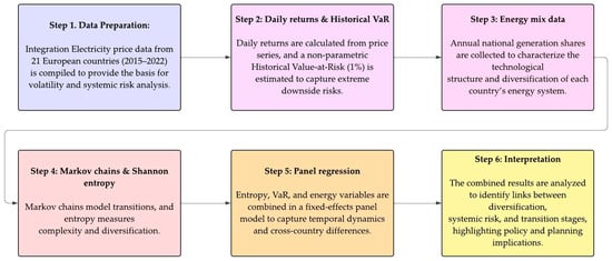
Figure 1.
Methodology Flowchart.
4. Results
This section presents the analysis of the results. In the first phase, descriptive analysis and electricity prices for the European countries included in the study are examined. Subsequently, the behavior of daily returns is analyzed to assess price stability over time. Based on the return series, the VaR is estimated for each country and for each year of the period considered. This indicator is relevant within the methodological approach, as it will be used as a response variable in the proposed model. In addition to the statistical and risk analysis, the European energy transition matrix is incorporated, which allows the observed patterns to be contextualized from a structural and cross-country perspective.
4.1. Descriptive Analysis
This section summarizes the main variables of the study using key descriptive statistics, including minimum, quartiles, median, mean, and maximum values. These indicators provide an overview of the distribution, central tendency, and variability of the data, establishing a basis for the interpretation and development of the model.
The descriptive statistics (Table 2) reveal substantial heterogeneity across variables. Energy prices such as Brent show relatively low dispersion and negative mean values, while Coal and Gas display much wider ranges with markedly higher maxima, indicating episodes of extreme price fluctuations. Nuclear also presents high variability, with a wide gap between the median and maximum values.
Table 2.
Summary variables.
The Entr_Vent indicators, which capture the variability of the transition matrix, generally exhibit low medians and means close to zero, with most observations concentrated at the lower bound, but with some higher values suggesting skewed distributions. Wind presents an unusual distribution, with a relatively low mean compared to an extremely high maximum, highlighting the presence of strong outliers. Finally, the VaR variable remains consistently negative, reflecting its role as a measure of downside risk.
The statistics indicate that the dataset combines relatively stable variables with others that display considerable dispersion and extreme values, reflecting the complexity and heterogeneity of the underlying processes.
Beyond their individual distributions, it is also important to determine the correlations that may exist among the variables, as this can provide additional insights into their relationships.
The correlation matrix (in Figure 2) shows heterogeneous relationships among the variables. The Entr_Vent series exhibit very strong positive correlations with each other, suggesting that they capture highly related dynamics. In contrast, traditional energy variables such as Brent, Coal, Gas, and Nuclear display weak or negligible correlations with the Entr_Vent group, indicating a low degree of direct association. Wind appears moderately correlated with Coal and Gas, while the VaR indicator maintains only weak connections across most variables. Overall, the plot highlights clusters of strongly interrelated variables alongside others that behave more independently.
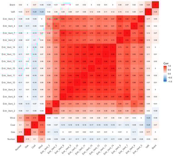
Figure 2.
Correlation Matrix.
4.2. Energy Price Analysis
Figure 3 shows how electricity prices, expressed in euros per megawatt-hour (EUR/MWh), evolved daily in 21 European countries between 2015 and 2022. The horizontal axis represents the passage of time, while the vertical axis captures price values, ranging from negative levels to over 800 EUR/MWh. Although the superposition of multiple curves makes it difficult to trace each trajectory separately, the figure clearly illustrates the main disruptions and structural changes that marked the European electricity market during this period. The visualization allows for the identification of both gradual trends and abrupt shocks, highlighting the complex interplay of market mechanisms and external factors in determining electricity prices.
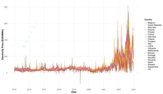
Figure 3.
Comparative Daily Electricity Prices in Europe by Country (2015–2022). Note: Daily data by country (EUR/MWh).
Between 2015 and 2020, electricity prices in Europe remained relatively stable, generally around 100 EUR/MWh, though occasional negative-price episodes appeared due to supply-demand imbalances. These events were linked to rising renewable penetration, system rigidity during surpluses, and marginalist market designs incentivizing generation under oversupply. Bublitz et al. (2017) highlight that the rapid expansion of wind and solar, combined with the planned phase-out of nuclear energy, significantly increased market sensitivity. They also emphasize that reliance on marginal fossil-fuel plants, together with cross-border market integration, propagated shocks across countries such as Germany, France, Italy, and Spain, amplifying short-term price volatility. Looking toward 2020, continued renewable growth and generation mix transitions were expected to sustain high price sensitivity and frequent volatility. Prokhorov and Dreisbach (2022) further argue that negative prices also result from high shutdown costs of conventional plants and exceptional demand anomalies, which push generators to maintain output even at sub-zero prices. These observations highlight the nuanced dynamics of electricity markets where even in periods of apparent stability, underlying stresses can produce extreme outcomes.
In 2021, an abrupt shift in price dynamics became evident. Countries began experiencing sustained increases and higher price volatility, a trend that intensified in 2022. Prices surged well beyond 400 EUR/MWh and, in extreme cases, reached or surpassed 800 EUR/MWh. In this phase, negative prices practically disappeared, replaced by sharp upward pressures. According to Martin-Valmayor et al. (2023), these developments stemmed from the steep rise in natural gas prices due to pandemic-related disruptions and the conflict in Ukraine, additional pressures in the CO2 emission rights market, and the persistence of the European marginalist pricing model. These conditions generated heightened uncertainty and sensitivity across the system, reflected in the greater density and interweaving of country price curves.
Energy price fluctuations in Europe thus emerge from the convergence of structural vulnerabilities and external shocks. Dependence on natural gas, despite its smaller share in total generation, disproportionately shapes price formation, while variations in fuel costs, carbon prices, and grid flexibility amplify the effects. Seasonal demand changes, limitations in storage, and the intermittent nature of renewables further increase the amplitude of price swings. At the same time, while negative prices resurfaced in 2023, they were less frequent and less intense, and a downward trend was observed, though average values remained above pre-2020 levels. Overall, distinct phases can be identified: an initial period of relative stability, followed by abrupt transitions toward extreme volatility with both upward and downward spikes. These shifts reveal not only the interaction between supply, demand, and market design but also the impact of external shocks, policy interventions, and the ongoing structural transformation of the European energy system (Zakeri et al., 2023). Understanding these drivers is critical, as volatility is primarily influenced by the marginal role of gas in price-setting, geopolitical tensions affecting supply, fluctuations in carbon costs, and the variable contribution of renewable sources to the energy mix.
4.3. Energy Price Returns Analysis
We study the behavior of daily electricity price returns to better understand the dynamics and stability of the European electricity market during the period analyzed. Unlike the analysis of absolute prices, the use of returns allows us to more accurately capture relative variations between consecutive days, which is essential for assessing the volatility and risks associated with each country. Logarithmic returns are calculated from daily price series, and their analysis allows us to identify common patterns, atypical events, and significant differences in the intensity of fluctuations across countries. This perspective not only provides information on market performance but also serves as a basis for estimating risk metrics such as VaR, which will be used later in the development of the model. By observing the evolution of returns, it is possible to detect periods of high instability linked to external events, as well as moments of relative calm that reflect more predictable system behavior.
Figure 4 illustrates the daily log returns of electricity prices for 21 European countries from 2015 to 2022. In the early years, many countries—such as Greece, Italy, Switzerland, and the UK—showed stable return patterns with low volatility and few extreme events. This suggests relatively resilient or less exposed electricity markets. However, from 2020 onward, countries like Sweden, Finland, Germany, and Denmark experienced a notable increase in price variability, marked by more frequent and extreme fluctuations. Sweden and Finland, in particular, showed strong signs of market stress, likely linked to growing renewable integration and external shocks.
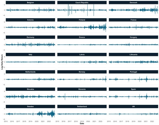
Figure 4.
Comparative Daily Electricity Returns Prices in Europe by Country (2015–2022). Note: Logarithmic daily returns.
The Czech Republic stands out for its early-period volatility (2016–2018), with extreme returns not seen elsewhere at that time. Meanwhile, countries like Estonia, Latvia, Lithuania, Norway, and the Netherlands experienced only mild increases in volatility, maintaining relatively stable price dynamics overall. Portugal, Spain, Slovakia, and Slovenia exhibited irregular patterns, with occasional spikes in returns but no clear long-term trend. Overall, three distinct groups emerge: (1) stable markets with low dispersion, (2) countries with growing volatility post-2020, and (3) markets with mixed or time-specific instability. These differences reflect varying levels of market integration, exposure to renewables, and policy environments across Europe.
4.4. VaR Estimation
To estimate VaR from the previously analyzed daily returns, a nonparametric approach based on the calculation of empirical quantiles is adopted. In this case, the objective is to identify the maximum expected loss, with a 99% confidence level, for each country and for each year of the study period. That is, the goal is to estimate the threshold below which the worst daily losses of the most extreme 1% of the return distribution are found, assuming that the observed data adequately capture the dynamics of the electricity market.
The procedure consists of grouping the returns by country and by year, and for each subset, calculating the 1st percentile (P1), which represents an approximation of the historical value at risk. This value robustly summarizes the behavior of the most adverse events within each calendar year and allows us to capture the magnitude of the most severe declines that could have occurred on a specific day. In this way, the database is transformed from a daily frequency to an annual aggregate structure by country, facilitating both temporal comparison and subsequent analysis in terms of accumulated risk and extreme behavior.
This methodology allows for the consolidation of a synthetic measure of daily electrical risk, transforming an extensive series of observations into a representative and comparable indicator that will be used as a dependent variable in the explanatory models developed in the following sections. The structure resulting from this aggregation process is presented below.
VaR translates financial risk into absolute losses by estimating the maximum potential loss a portfolio could incur over a specific time horizon at a given confidence level (Halkos & Tsirivis, 2019). For example, a daily 99% VaR indicates the loss that will only be exceeded on 1% of trading days, providing a concrete monetary measure of extreme downside risk. In the energy sector, this allows companies and investors to quantify exposure to price fluctuations and volatility in energy commodities, supporting informed decisions on hedging and risk management. Figure 5 shows the annual 1% VaR of daily electricity price returns in 21 European countries from 2015 to 2022, highlighting extreme risk episodes, variability across countries, and rising risk trends in recent years. Belgium presents a relatively stable extreme risk profile between 2015 and 2020, with values between −0.37 and −0.58, but experiences a sharp deterioration in 2021 (VaR = −1.17) and a slight improvement in 2022 (−0.87). In the Czech Republic, 2016 was notable for a particularly severe extreme risk event (VaR = −2.60), the most pronounced in the country, while the other years showed moderate fluctuations. Denmark showed an upward risk trajectory starting in 2018, reaching a VaR of −2.49 in 2022, indicating a progressive accumulation of vulnerability.
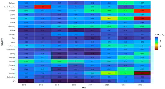
Figure 5.
VaR Returns Prices in Europe by Country (2015–2022). Note: Heatmap of 1% VaR of daily electricity returns.
Estonia and Finland shared an upward risk trend starting in 2020, but Finland exhibited the most extreme values of all countries in 2022 (VaR = −2.66), suggesting high exposure to extreme events in the final stage of the period. France, on the other hand, maintained a narrower range of variation, with VaR fluctuating between −0.48 and −0.62, reflecting greater relative stability in its extreme return dynamics. Germany, one of the largest electricity markets, shows a sustained deterioration in VaR between 2017 and 2020, reaching a level of −1.15 in 2020 and maintaining high values in subsequent years. In contrast, Greece, Hungary, and Italy present more moderate profiles, with 1% VaR typically ranging between −0.2 and −0.6, without registering abrupt year-on-year variations, suggesting lower exposure to severe shocks. Latvia and Lithuania show somewhat more volatile values, with Lithuania standing out in 2020 at −1.06 and in 2021 at −0.96, which could be linked to regional tensions or structural market conditions.
In the case of the Netherlands, the VaR remains between −0.24 and −0.67, without extreme episodes, while Norway shows a progressive deterioration, reaching a value of −1.11 in 2022, similar to that of more volatile countries. Portugal shows a more severe VaR in 2016 and 2022, although it remains within a lower range than the Nordic countries. Slovakia, for its part, shows consistently low values starting in 2017, with a minimum VaR of −1.21 in that year and a persistently high risk in subsequent years.
Slovenia, Spain, and Sweden show upward VaR trajectories, with Sweden being particularly notable, culminating with a VaR of −2.82 in 2022, the most negative of the group, indicating a significant increase in the risk of extreme events. Finally, Switzerland maintains relatively stable values, with a VaR ranging between −0.32 and −0.65, while the United Kingdom presents one of the most moderate profiles of the group, with a VaR consistently close to −0.3 and no notable extreme events. In terms of time, a common trend is observed across countries: between 2015 and 2019, the VaR remained mostly at moderate levels (generally above −0.6), suggesting a less frequent sharp decline in daily prices. Beginning in 2020, however, there was a general increase in the magnitude of extreme risk, with multiple countries recording VaRs below −1.0. This intensification of risk persisted and worsened in 2022, when the most negative values were observed in most Nordic and Central European countries.
This outlook reveals not only structural differences between national electricity markets, but also a progressive transformation in the intensity of risks during the period analyzed, which is particularly marked in the final phase of the time horizon considered.
4.5. Energy Transition Matrix
The structure of energy production reflects the combination of sources used to meet a country’s energy demand, providing insights into its overall composition and the degree of dependence on specific resources such as fossil fuels, hydropower, or non-conventional renewables. This composition is shaped by each nation’s economic, geographic, and technological context. In this regard, the following Figure 6 presents the evolution of different energy production structures over time, highlighting which sources predominate in each country during different periods and offering a comparative view of the overall energy structure in Europe.
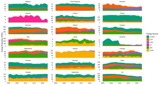
Figure 6.
Energy Production Matrix in Europe.
After obtaining the country–year details, the overall participation of the different energy production sources is calculated (Table 3), showing their percentage contribution. For each country, the shares of all energy sources add up to 100%, allowing a standardized comparison of the energy production structure across nations.
Table 3.
Energy Production Participation Matrix in Europe (%): Each Row Sums to 100%.
To construct the European-level energy transition matrix, the predominant source of electricity generation in each country is identified for each year of the period analyzed. This estimate is based on determining, for each country and year, the source with the highest annual generation volume, understood as the one with the highest production value among all available technologies.
This approach allows each country to be classified annually according to its primary dependence on a specific energy source (e.g., hydroelectric, nuclear, thermal, or intermittent renewable energy), which facilitates monitoring structural changes in the regional energy mix. Based on this information, a dynamic matrix is created that captures, in aggregate, the evolution of the dominant source in each country over time, thus providing an empirical basis for comparative analysis of the energy transition in Europe.
Figure 7 presents the transition matrix for the 21 European countries included in the analysis. To construct it, we used a database organized with countries as rows and years of analysis as columns. At each intersection, the dominant energy source was identified, providing the main source of production for each country and each year. Based on this information, Figure 7 illustrates the transitions in energy sources across all countries throughout the study period. Specifically, the transition matrix was calculated from one year to the next, allowing us to establish both the initial and the final periods. The left axis represents the dominant sources in an initial year (“Start”), while the right axis shows the dominant source in a subsequent year (“End”). The thickness of each band indicates the number of countries that have undergone a transition between the respective sources.
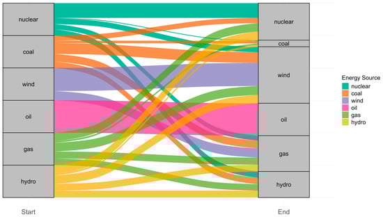
Figure 7.
Energy Source Transition Matrix in Europe: Sankey Diagram of Dominant Technologies Over Time.
The graphical analysis reveals several relevant patterns. Initially, a significant number of transitions are observed from fossil fuel sources, such as coal and oil, to cleaner technologies such as wind and hydropower. This behavior suggests a general trend toward decarbonization of national energy matrices, in line with European climate change commitments and energy transition goals.
Moreover, some technologies show remarkable persistence. This is the case of nuclear, hydroelectric, and, to a lesser extent, wind energy, which in several countries have maintained their position as the dominant source throughout the period considered. These stable trajectories indicate that, despite advances in new technologies, certain countries maintain a high structural dependence on specific sources, whether due to comparative advantages, installed capacity, or energy policy decisions. Additionally, cross-flows are identified that reflect more complex or less systematic changes. For example, some countries have transitioned from renewable technologies to fossil or intermediate sources such as gas, which could respond to specific situations such as supply crises, failures in the integration of variable energies, or changes in regulatory frameworks.
From this aggregated representation, it is evident that the energy transition in Europe does not follow a single path, but rather responds to multiple national dynamics. In this sense, and based on this analytical logic, an individual energy transition matrix will be constructed for each country, allowing a more detailed observation of the specific evolution of each electricity system. This methodology will also be applied to different time windows of historical data (e.g., rolling five-year periods) to capture patterns of change that may vary depending on the stage of the transition process.
This approach will not only identify dominant technological trajectories by country, but also characterize the speed, stability, or reversibility of energy transition processes based on the national and temporal context. This will advance a more granular and comparative understanding of the structural transformation of European electricity systems.
4.6. Empirical Model
The estimation of the Shannon index follows the same logic used in the analysis of the energy transition matrix, with one fundamental difference: instead of constructing a single aggregated matrix for all of Europe, country-specific transition matrices are generated. The objective is to capture and assess the degree of variability in the electricity generation structure at the national level, observing how the main source of generation changes over time. This procedure involves constructing an extensive set of transition matrices, one for each country, each year, and for different historical analysis time windows. From these matrices, the Shannon index is calculated as a measure of entropy associated with the distribution of transition probabilities between energy sources. This metric makes it possible to quantify the level of dispersion or uncertainty in each country’s transition trajectories. Interpretatively, low values of the Shannon index, close to zero, indicate that the country’s energy matrix is relatively stable, with high persistence in its dominant source of generation. On the other hand, high values reflect greater heterogeneity in technological transitions, suggesting a more dynamic or transforming electricity system. This indicator, by capturing the degree of structural variability in the national energy matrix, is incorporated as an explanatory covariate in the proposed model, allowing us to assess the extent to which the complexity or instability of the energy system is related to the estimated electricity risk.
Once the database containing detailed information on the energy mix of different European countries was consolidated, multiple balanced panel data models with fixed effects were estimated. In total, more than 500.000 models were evaluated, of which only 21 were found to be statistically significant. We only include windows of length 5, 6 and 7, because they are significant.
The set of models presented (Table 4) analyzes different combinations of variables associated with energy sources (Brent, coal, wind, and nuclear), together with entropy measures calculated for different time windows (Entr_Vent_5, Entr_Vent_6, and Entr_Vent_7), with the purpose of modeling VaR under a fixed-effects panel framework. Some models (1, 3, 4, and 9) consider a single source, while others (21, 22, 55, 192, and 1160) combine several sources to capture interactions or compound effects. The variables hydro, solar and oil do not appear in the table since, although they were initially considered in the modeling stage, they did not prove to be statistically significant. Therefore, models that integrate variables related to technological or structural transition processes (27, 28, 29, and 215) are also included, reflecting the interest in understanding the impact of changes in the configuration of the energy system.
Table 4.
Significant Fixed-Effects Panel Models.
However, among the models that incorporate entropy variables (Table 5), Model 215 performs best according to the AIC and BIC information criteria. This model includes Brent, coal, and the entropy calculated in the Entr_Vent_7 window as explanatory variables. For this reason, Model 215 is selected as the most appropriate. This methodology seeks to assess the degree of variability and diversification in the national energy mix, observing how the predominant source of electricity generation changes or remains the same over time. This approach is particularly valuable for understanding stability, dependence on certain energy resources, and the pace of adaptation toward more sustainable sources in specific contexts, thus contributing to a more accurate understanding of the energy transition process from a national and temporal perspective.
Table 5.
Performance Metrics of Selected Fixed-Effects Panel Models.
The estimated model corresponds to a fixed effects (“within”) regression applied to a balanced panel including 21 countries over 8 periods, for a total of 168 observations. The main objective is to identify how variables linked to energy market behavior, specifically Brent oil and Coal price volatility, along with the entropy indicator Entr_Vent_7, influence the energy VaR (Table 6), understood as a proxy for systemic risk within national energy systems.
Table 6.
Results of the balanced panel data model 215 estimation with fixed effects.
The model attains an R-squared of 0.224, explaining 22.4% of the variability in energy risk. Although modest, this level of fit is reasonable given the complexity of systemic energy risk. The F statistic (13.89, p < 0.000001) further confirms the overall significance of the specification, while the signs and significance of the coefficients reinforce its explanatory value.
The results presented in Table 6 were obtained prior to performing the Hausman test, whose results are reported in Appendix C. Robustness tests, detailed in Appendix D, Appendix E and Appendix F, provide additional support for the model’s validity. The Breusch–Pagan LM tests confirmed the suitability of the fixed-effects specification and the presence of significant individual effects. Furthermore, the Driscoll–Kraay and clustered robust errors confirmed the significance of Brent, Coal, and Entr_Vent_7 across alternative error structures. Taken together, these findings indicate that, despite its limited predictive power, the model provides consistent and reliable evidence on the structural determinants of electricity risk volatility (VaR).
The specification tests further confirm that the fixed-effects model adequately controls for unobserved heterogeneity and mitigates potential endogeneity, ensuring the consistency and robustness of the estimated coefficients.
From an economic perspective, the Brent oil price represents one of the main global benchmarks in hydrocarbon markets. The estimate obtained reveals that its volatility has a positive and highly significant effect on energy risk (coefficient: 2.14; p < 0.001). This finding suggests that oil price shocks continue to substantially affect the stability of energy systems, especially in countries that depend on imported oil. In contexts of high global uncertainty, such as geopolitical conflicts, OPEC decisions, or financial crises, fluctuations in Brent can alter both generation costs and countries’ energy planning. On the other hand, the price of coal (Coal), although less influential in terms of magnitude, also shows a positive and significant effect (coefficient: 0.0018; p ≈ 0.031). This result highlights that, despite the global discourse geared toward decarbonization, coal continues to play an important role in the energy mix of many economies, particularly those with legacy thermal infrastructure. Exposure to risk derived from its volatility remains a factor that cannot be underestimated in the assessment of energy security.
One of the most interesting contributions of the model is the inclusion of the entropy indicator calculated over a 7-period window (Entr_Vent_7). This indicator seeks to capture the complexity, dispersion, or structural uncertainty of the energy system from a dynamic perspective. Unlike a static measure of diversity, this version incorporates a temporal dimension, assessing how the composition of the energy mix has changed over a recent rolling window. The positive coefficient (0.20; p ≈ 0.036) suggests that as the entropy of the energy system increases—that is, when the system exhibits greater technological diversity and the relative share of multiple sources—the energy value at risk also tends to increase.
This finding invites an important reflection: although source diversification is a key objective for energy sustainability, it does not always translate into lower risk exposure, at least in the short term. In fact, a more diverse energy matrix can also be more complex to operate, especially if institutional and technical frameworks do not evolve at the same pace. In this sense, the energy transition brings with it new forms of uncertainty that must be carefully managed.
This model shows that energy risk depends not only on external factors such as oil and coal price volatility, but also on internal transformations in the structure of energy systems. To complement the results obtained from the model selected in Table 6, we propose re-estimating the same specification, but this time using C-VaR as the response variable instead of VaR, as originally defined (Acerbi & Tasche, 2002). The outcomes of this alternative estimation are presented in Appendix G. Furthermore, to extend the analysis, we implement a two-way fixed-effects model that simultaneously incorporates both country and year dummy variables. The aim of this approach is to evaluate how the model behaves when controlling for both country-specific and time-specific effects, thereby providing a more precise understanding of the underlying patterns in the data. By jointly including these dummies, the model captures unobserved heterogeneity across countries as well as temporal shocks that may affect the results. The outcomes of this extended model are presented below:
The results (Table 7) show that Brent has a strong and statistically significant positive effect at the 5% level, while Coal is not significant. Some year dummies (e.g., 2021) are significant, with 2017 and 2020 marginally so at the 10% level, suggesting modest temporal variation. Several country effects are also significant: Germany exhibits a marked negative impact, while Greece, Italy, Hungary, Norway, Switzerland, the Netherlands, Denmark, the Czech Republic, Slovakia, and the UK display significant differences relative to the baseline.
Table 7.
Two-way fixed-effects model with country and year dummies together.
However, as Gujarati and Porter (2010) notes, the introduction of a large number of dummy variables can substantially reduce degrees of freedom, weaken statistical power, and increase the risk of multicollinearity, which hinders precise parameter estimation. Moreover, variables with little variation over time may have their effects absorbed by unit-specific components of the model. These methodological constraints help explain why some coefficients, despite their theoretical relevance, do not appear as statistically significant in the estimates.
5. Discussion
This study analyzes electricity risk in Europe by combining quantitative analysis, structural insight, and temporal evolution. Using daily price and return data from 2015 to 2022 and estimating a fixed-effects panel model, the analysis connects short-term market volatility with long-term shifts in energy system configurations. A structural break is identified in 2021, characterized by extreme price spikes (up to 800 EUR/MWh) associated with global events such as the war in Ukraine, the gas crisis, and CO2 market pressures. The VaR estimates indicate heterogeneous effects across countries, with Finland, Sweden, and Denmark exhibiting the highest systemic risk levels in 2022.
Shannon entropy, derived from country-level technological transition matrices, is employed to represent the structural complexity of energy mixes. The results show a positive and statistically significant relationship between entropy and VaR, which suggests that high levels of diversification reflect ongoing transitions and operational complexity that may increase uncertainty if not properly managed. The sensitivity of VaR to Brent oil and coal prices indicates that fossil fuel markets continue to influence electricity price formation and backup cost structures, even in the presence of renewable integration. These results point to the need for energy planning frameworks that incorporate both diversification and resilience metrics, accounting for integration of intermittent renewables, smart grids, storage, and market flexibility.
An additional insight emerging from the entropy–VaR analysis relates to the potential stages of the energy transition and their associated risk profiles. Although the 2015–2022 period is relatively short and countries are not synchronized in their transition trajectories, the combination of entropy values and systemic risk estimates offers clues about different phases. Higher entropy values often signal more dynamic reconfigurations of the energy mix, which can be interpreted as early or transitional stages, where technological shifts are frequent and operational uncertainty is elevated. In our results, countries such as Finland, Sweden, and Denmark exhibit both high entropy and elevated VaR in recent years, suggesting active and potentially volatile phases of transition. Conversely, countries such as Greece and the United Kingdom display low entropy levels and more stable VaR profiles, consistent with more consolidated or long-term stable stages in their energy systems. While this interpretation is qualitative, it provides a conceptual link between the empirical indicators and the broader theory of energy transition stages, complementing the quantitative findings of this study. At the same time, the results also reveal cases where the energy system remains structurally locked in a single dominant source of generation. For instance, Estonia shows a persistent reliance on oil as its main source across short-, medium-, and long-term horizons, which results in entropy values that converge to zero. This indicates a severe restriction in the diversification of its energy mix over time. A similar phenomenon is observed for France, where nuclear energy consistently dominates the generation structure. Although the primary energy source differs from Estonia, the outcome is comparable, as France also records zero entropy throughout the period, reflecting a highly stable but non-diversified configuration.
Building on the evidence that higher entropy—representing greater diversity and dynamism in the energy portfolio—correlates with elevated systemic risk, policymakers should adopt strategies specifically designed for high-entropy environments. These may involve: (i) implementing capacity mechanisms or strategic reserves to guarantee supply security during accelerated shifts in generation structures; (ii) offering focused incentives for storage systems and demand-side response to cushion variability and limit dependence on costly peak generation; (iii) strengthening cross-border interconnections and regional balancing arrangements to absorb fluctuations and reduce country-specific volatility; and (iv) redesigning market rules to reward flexibility and ancillary services, ensuring that system stability is valued alongside energy output. Taken together, these measures can reframe technological diversity from a near-term source of instability into a foundation for long-term resilience.
6. Conclusions
The evidence presented in this study demonstrates that the energy transition in Europe does not follow a uniform or linear pattern. Each country exhibits unique structural dynamics and differentiated strategies, which implies that energy risk cannot be adequately assessed through aggregate analysis alone. Instead, it requires a granular approach that reflects the specific configuration and evolution of each national electricity system.
The incorporation of the Shannon entropy index represents a significant methodological contribution, as it enables the quantification of structural variability in the energy mix over time. Countries with low entropy values tend to maintain a dominant generation source, reflecting greater stability, whereas higher entropy levels indicate more dynamic transitions and increased operational uncertainty. This measure therefore provides a structural lens through which the pace and complexity of the transition can be evaluated.
When combined with financial measures such as Value at Risk (VaR), the entropy index offers a powerful dual perspective linking technological change with systemic financial exposure. This integration of technological structure and market behavior enhances the understanding of energy risk in Europe and supports the development of strategies aimed at mitigating financial vulnerability in electricity markets. It also provides an empirical basis for anticipating periods of heightened volatility and for designing more resilient investment and policy approaches.
Constructing transition matrices through rolling time windows further captures not only the composition of national energy systems but also their speed of change. This method allows for the identification of phases of acceleration, stagnation, or reversal in the transition process and reveals how countries respond to external shocks such as geopolitical crises, price volatility, or regulatory adjustments. Recognizing these dynamics facilitates the implementation of more effective risk mitigation measures, reducing potential financial losses during periods of structural or market instability.
The findings also underscore the importance of advancing probabilistic modeling frameworks and composite vulnerability indices that integrate financial risk, structural variability, and technological resilience. Such analytical tools would improve the anticipation and management of systemic challenges, contributing to the mitigation of financial risk in European energy markets by offering actionable guidance for both investment and policy decisions.
Strategically, accelerating the adoption of renewable energy and strengthening domestic capacity for clean technology production are essential steps. Reducing dependence on fossil fuels and on suppliers from geopolitically unstable regions enhances energy security and environmental sustainability. Equally important is the alignment of the financial system with transition objectives, ensuring that capital flows are redirected toward sustainable sectors and that the process of structural adjustment occurs in an orderly and stable manner.
Investment and portfolio diversification strategies should therefore account for the aggregate share of renewables as well as the specific contribution of each technology, transaction costs, and extended investment horizons. Considering these dimensions strengthens portfolio resilience amid structural and cyclical transformations in energy markets, reinforcing the capacity of both policymakers and investors to design transitions that are adaptive, resilient, and capable of balancing sustainability objectives with the long-term stability and reliability of the European energy system.
Several limitations should be considered when interpreting these findings. The Shannon entropy index, while suitable for capturing the structural complexity of national energy matrices, does not fully incorporate technological and institutional factors such as capacity factors, intermittency, or regulatory frameworks. The use of historical Value at Risk (VaR) with panel data provides a coherent approach for systemic risk assessment, but its assumptions of stable return distributions and historical dependence limit its ability to capture nonlinear dynamics or extreme events, including structural breaks or regime shifts. Similarly, the reliance on annual production data to construct the energy matrix, although facilitating cross-country comparability, may omit short-term fluctuations that influence real-time price volatility. In addition, the use of Markov chains to identify transition patterns is based on time-homogeneous assumptions, which may not adequately represent periods characterized by rapid technological or geopolitical change.
Future research could benefit from extending the analysis toward more flexible and adaptive modeling approaches such as stochastic simulations or Bayesian frameworks that better capture the uncertainty and complexity associated with energy transitions. Future extensions of this study will integrate entropy measures computed from the full distribution of generation shares, providing a more nuanced view of diversification patterns and complementing the current dominant-source approach.
Author Contributions
Conceptualization, O.W.O.-C. and O.J.-B.; methodology, O.W.O.-C., O.J.-B. and D.F.M.-D.; validation, O.W.O.-C. and O.J.-B.; formal analysis, O.W.O.-C., O.J.-B. and D.F.M.-D.; investigation, O.W.O.-C. and D.F.M.-D.; data curation, O.W.O.-C.; writing—original draft preparation, O.W.O.-C. and O.J.-B.; writing—review and editing, O.W.O.-C., O.J.-B. and D.F.M.-D.; visualization, O.W.O.-C. and O.J.-B. All authors have read and agreed to the published version of the manuscript.
Funding
This research received no external funding.
Institutional Review Board Statement
Not applicable.
Informed Consent Statement
Not applicable.
Data Availability Statement
Data are contained within paper.
Conflicts of Interest
The authors declare no conflicts of interest.
Appendix A. Energy Balance Structure 2022
| Country | A | B | C | D | E | F | G | H | I | J | K | L | M |
| Belgium | 683.7 | 3410.9 | −1572.8 | 2119.0 | −419.9 | −9.5 | 1523.7 | 399.8 | 358.3 | 295.9 | 165.2 | 304.6 | 7258.8 |
| Czech Rep. | 1061.1 | 1004.3 | −272.2 | 1741.3 | −483.1 | 0.4 | 1109.2 | 275.6 | 286.8 | 286.8 | 119.6 | 140.4 | 5270.1 |
| Denmark | 399.1 | 730.7 | −422.6 | 649.7 | −26.5 | −6.4 | 536.4 | 96.2 | 166.3 | 155.6 | 80.1 | 38.2 | 2396.8 |
| Estonia | 196.5 | 114.0 | −100.3 | 201.0 | −48.4 | 0.0 | 119.8 | 15.0 | 35.6 | 40.4 | 19.1 | 9.7 | 602.3 |
| Finland | 809.5 | 928.4 | −368.9 | 1321.7 | −235.4 | −3.5 | 996.8 | 411.6 | 160.8 | 207.4 | 121.1 | 95.9 | 4445.5 |
| France | 4355.6 | 6106.1 | −1300.8 | 8841.1 | −2435.9 | −23.4 | 5903.0 | 1127.3 | 1866.6 | 1417.1 | 828.1 | 664.0 | 27,348.6 |
| Germany | 4008.0 | 9760.1 | −1620.8 | 11,355.9 | −1743.7 | −59.3 | 8760.9 | 2238.7 | 2126.7 | 2333.4 | 1058.9 | 1003.2 | 39,222.0 |
| Greece | 208.3 | 1578.7 | −782.6 | 856.8 | −145.8 | 31.1 | 654.0 | 107.4 | 254.6 | 176.7 | 73.3 | 42.0 | 3054.6 |
| Hungary | 451.0 | 851.1 | −158.4 | 1074.8 | −180.5 | 0.5 | 828.8 | 181.1 | 220.0 | 242.4 | 78.9 | 106.5 | 3696.1 |
| Italy | 1337.7 | 6368.3 | −1385.1 | 5958.7 | −973.0 | 36.1 | 4768.0 | 1039.0 | 1535.9 | 1225.5 | 593.0 | 374.6 | 20,878.7 |
| Latvia | 122.3 | 161.2 | −87.9 | 177.4 | −7.5 | 0.0 | 164.0 | 37.9 | 42.9 | 46.6 | 24.0 | 12.7 | 693.5 |
| Lithuania | 81.7 | 593.0 | −374.4 | 287.9 | −8.2 | 1.8 | 247.7 | 39.8 | 87.6 | 61.9 | 26.0 | 32.3 | 1077.1 |
| NLD (*) | 999.3 | 7812.3 | −5190.2 | 2650.0 | −293.2 | −23.0 | 2072.6 | 523.4 | 384.7 | 347.3 | 252.5 | 564.8 | 10,100.4 |
| Norway | 9045.2 | 482.6 | −8420.2 | 1057.8 | −10.6 | 0.9 | 881.8 | 267.0 | 214.9 | 161.0 | 119.2 | 119.7 | 3919.2 |
| Portugal | 246.7 | 907.8 | −213.6 | 851.3 | −97.4 | −11.2 | 679.4 | 188.0 | 240.4 | 111.5 | 77.1 | 62.4 | 3042.4 |
| Slovakia | 290.5 | 684.1 | −199.7 | 702.2 | −148.4 | 5.9 | 461.8 | 135.0 | 112.3 | 109.5 | 53.0 | 52.1 | 2258.4 |
| Slovenia | 128.8 | 274.0 | −129.8 | 268.7 | −58.7 | 0.0 | 201.7 | 49.5 | 82.6 | 41.3 | 17.4 | 11.0 | 886.3 |
| Spain | 1453.6 | 5287.1 | −1297.3 | 4815.0 | −889.4 | −71.6 | 3408.9 | 745.4 | 1346.8 | 587.3 | 391.2 | 338.2 | 16,115.2 |
| Sweden | 1496.4 | 1347.8 | −803.0 | 1899.7 | −436.3 | −15.5 | 1311.4 | 472.4 | 276.3 | 295.7 | 176.5 | 90.6 | 6112.0 |
| Switzerland | 499.9 | 620.6 | −132.0 | 952.2 | −205.1 | −0.2 | 703.2 | 139.5 | 220.8 | 192.9 | 120.6 | 29.4 | 3141.8 |
| UK | 4325.0 | 5720.6 | −3189.9 | 6406.4 | −1041.1 | −64.4 | 4759.1 | 869.7 | 1600.6 | 1323.4 | 541.5 | 423.9 | 21,674.9 |
| A: Production (PJ). B: Imports (PJ). C: Exports (PJ). D: Total energy supply (PJ). E: Electricity, CHP and heat plants (PJ). F: Oil refineries, transformation (PJ). G: Total final consumption (PJ). H: Industry (PJ). I: Transport (PJ). J: Residential (PJ). K: Commercial and public services (PJ). L: Other final consumption (PJ). M: Sum by row (PJ). (*) Netherlands. Note: 1 PJ = 0.278 TWh. | |||||||||||||
Appendix B. Definitions Columns Appendix A
| Term | Meaning |
| Production (PJ) | Primary energy produced domestically (coal, oil, gas, renewables, nuclear, hydro, solar, geothermal, etc.), net of impurities. |
| Imports (PJ) | Energy entering the country’s borders. Includes crude oil, gas, and electricity crossing borders; excludes fuel in transit. |
| Exports (PJ) | Energy leaving the country’s borders. Includes crude oil, oil products, gas, and electricity delivered abroad; excludes fuel in transit. |
| Total Energy Supply (TES) | Energy available domestically: Production + Imports—Exports—Bunkers ± Stock changes. |
| Electricity, CHP & Heat Plants (PJ) | Energy generated by electricity-only plants, combined heat and power (CHP) plants, and heat-only plants (for sale or own use). |
| Oil Refineries, Transformation (PJ) | Positive = finished oil products; Negative = crude oil, NGLs, or feedstocks used as refinery inputs. |
| Total Final Consumption (PJ) | Energy actually consumed by end-users (households, industry, transport, services). Excludes energy used for transformation and production processes. |
| Industry (PJ) | Energy used in industrial sectors (iron & steel, chemicals, metals, machinery, construction, textiles, etc.), excluding transport. |
| Transport (PJ) | Energy consumed in all transport activities (road, rail, air, pipelines) regardless of sector. |
| Residential (PJ) | Household energy use, excluding fuels for transport. |
| Commercial & Public Services (PJ) | Energy use by service sectors (retail, offices, education, health, government, etc.). |
| Other Final Consumption (PJ) | Agriculture, forestry, fishing, non-specified uses, and non-energy purposes. |
Appendix C. Hausman Test
| chisq = 12.146, df = 3, p-value = 0.006898 |
| alternative hypothesis: one model is inconsistent |
Appendix D. Lagrange Multiplier Test—(Breusch-Pagan)
| chisq = 103.55, df = 1, p-value < 2.2 × 10⁻¹⁶ |
| alternative hypothesis: significant effects |
Appendix E. t-Test with Driscoll–Kraay Robust Standard Errors
| Variable | Estimate | Std. Error | p-Value |
| Brent | 2.1394.815 | 0.3836677 | 1.177 × 10⁻⁷ |
| Coal | 0.0018272 | 0.0007208 | 0.01232 |
| Entr_Vent_7 | 0.2004578 | 0.0927736 | 0.03237 |
Appendix F. t-Test with Heteroskedasticity-Consistent Clustered Standard Errors (By Group)
| Variable | Estimate | Std. Error | p-Value |
| Brent | 2.1394.815 | 0.4030848 | 4.109 × 10⁻⁷ |
| Coal | 0.0018272 | 0.0002882 | 2.801 × 10⁻⁹ |
| Entr_Vent_7 | 0.2004578 | 0.0644305 | 0.002244 |
Appendix G. Model with Response C-VaR
| Variable | Coefficient | Std. Error | p-Value |
| Brent | 0.8266530 | 1.5398211 | 0.592200 |
| Coal | 0.0160184 | 0.0056922 | 0.005576 |
| Entr_Vent_7 | 0.2284695 | 0.6363852 | 0.720113 |
Appendix H. Model GARCH(1,1)-VaR vs. VaR (1%) by Country

Appendix I. Backtesting Results of GARCH(1,1)-VaR Models: Kupiec (LRuc) and Christoffersen (LRcc) Tests by Country
| Country | Lruc-Test | LRcc-Test |
| Belgium | 0.000 | 0.000 |
| Czech Rep. | 0.941 | 0.969 |
| Denmark | 0.000 | 0.000 |
| Estonia | 0.021 | 0.056 |
| Finland | 0.002 | 0.001 |
| France | 0.148 | 0.312 |
| Germany | 0.000 | 0.000 |
| Greece | 0.059 | 0.142 |
| Hungary | 0.021 | 0.056 |
| Italy | 0.148 | 0.312 |
| Latvia | 0.007 | 0.019 |
| Lithuania | 0.059 | 0.142 |
| NLD (*) | 0.001 | 0.002 |
| Norway | 0.007 | 0.019 |
| Portugal | 0.002 | 0.006 |
| Slovakia | 0.148 | 0.312 |
| Slovenia | 0.328 | 0.572 |
| Spain | 0.002 | 0.006 |
| Sweden | 0.000 | 0.000 |
| Switzerland | 0.059 | 0.142 |
| UK | 0.636 | 0.849 |
| (*) Netherlands. | ||
Appendix J. AIC and BIC
| Model | AIC | BIC |
| VaR~ Brent | −690.23 | −687.10 |
| VaR~ Brent + Coal | −694.62 | −688.37 |
| VaR~ Brent + Coal + Entr_Vent_7 | −697.75 | −688.38 |
Appendix K. Hansen–Sargan Test of Overidentifying Restrictions and AR(2)
| Sargan | AR (2) |
| 0.48781 | 0.98095 |
References
- Acerbi, C., & Tasche, D. (2002). On the coherence of expected shortfall. Journal of Banking & Finance, 26(7), 1487–1503. [Google Scholar] [CrossRef]
- Adamko, P., Spuchľáková, E., & Valášková, K. (2015). The history and ideas behind VaR. Procedia Economics and Finance, 24, 18–24. [Google Scholar] [CrossRef]
- Barragán-Ocaña, A., Cecilio-Ayala, E., Silva-Borjas, P., Cortés-Ruiz, J. A., & Hernandez-Cardona, E. Y. (2025). Policies and sustainable energy transition in the global environment: Challenges for Latin America. Heliyon, 11(6), e42295. [Google Scholar] [CrossRef]
- Baruník, J., & Čech, F. (2021). Measurement of common risks in tails: A panel quantile regression model for financial returns. Journal of Financial Markets, 52, 100562. [Google Scholar] [CrossRef]
- Bollerslev, T. (1986). Generalized autoregressive conditional heteroskedasticity. Journal of Econometrics, 31(3), 307–327. [Google Scholar] [CrossRef]
- Božičević Vrhovčak, M., & Malbašić, B. (2023). Unlocking the value of aggregated demand response: A survey of European electricity markets. Energies, 16(17), 6386. [Google Scholar] [CrossRef]
- Böhringer, C., & Löschel, A. (2006). Computable general equilibrium models for sustainability impact assessment: Status quo and prospects. Ecological Economics, 60(1), 49–64. [Google Scholar] [CrossRef]
- Bublitz, A., Keles, D., & Fichtner, W. (2017). An analysis of the decline of electricity spot prices in Europe: Who is to blame? Energy Policy, 107, 323–336. [Google Scholar] [CrossRef]
- Chen, L. J., Lu, L. J., Tai, M. Y., Hu, S. W., & Wang, V. (2014). Energy structure, energy policy, and economic sustain-able development. International Review of Economics & Finance, 34, 203–210. [Google Scholar] [CrossRef]
- Cooray, A., Shahbaz, M., Kuziboev, B., & Çatık, A. N. (2025). Mitigating energy risk through energy sources diversi-fication. Journal of Environmental Management, 380, 124955. [Google Scholar] [CrossRef]
- Das, A., & Schlüter, S. (2025). Gaussian process regression with a hybrid risk measure for dynamic risk management in the electricity market. Risks, 13(1), 13. [Google Scholar] [CrossRef]
- Datta, J., & Das, D. (2025). Risk-constrained energy management of multi-energy multi-microgrids system with integrated demand response using hybrid risk assessment approach. Energy, 331, 136638. [Google Scholar] [CrossRef]
- Dincer, I., & Abu-Rayash, A. (2020). Chapter 3—Energy systems. In I. Dincer, & A. Abu-Rayash (Eds.), Energy sustainability (pp. 59–92). Academic Press. [Google Scholar] [CrossRef]
- Ewald, C. O., Huang, C., & Ren, Y. (2024). On the effects of physical climate risks on the Chinese energy sector. Journal of Risk and Financial Management, 17(10), 458. [Google Scholar] [CrossRef]
- Fitriani, E., Hikmah, Y., & Hikmah, I. R. (2024). Comparison of value at risk using historical and monte carlo methods on pt xyz stock portofolio. Jurnal Administrasi Bisnis Terapan, 6(2), 1. [Google Scholar] [CrossRef]
- Gujarati, D. N., & Porter, D. C. (2010). Econometria. Mc-Graw Hill Interamericana. [Google Scholar]
- Halkos, G. E., & Tsirivis, A. S. (2019). Value-at-risk methodologies for effective energy portfolio risk management. Economic Analysis and Policy, 62, 197–212. [Google Scholar] [CrossRef]
- Han, F., & Fu, L. (2025). Maximizing profitability in integrated energy markets: A novel framework for multi-faceted energy trading. Electric Power Systems Research, 238, 111171. [Google Scholar] [CrossRef]
- Hirth, L. (2013). The market value of variable renewables: The effect of solar wind power variability on their relative price. Energy Economics, 38, 218–236. [Google Scholar] [CrossRef]
- Hou, Y., Leng, X., Peng, L., & Zhou, Y. (2024). Panel quantile regression for extreme risk. Journal of Econometrics, 240(1), 105674. [Google Scholar] [CrossRef]
- Huang, Z., Duan, J., Zhang, C., & Gong, W. (2025). SDELP-DDPG: Stochastic differential equations with Lévy processes-driven deep deterministic policy gradient for portfolio management. Expert Systems with Applications, 273, 126822. [Google Scholar] [CrossRef]
- Igliński, B., Kiełkowska, U., Mazurek, K., Drużyński, S., Pietrzak, M. B., Kumar, G., Veeramuthu, A., Skrzatek, M., Zinecker, M., & Piechota, G. (2024). Renewable energy transition in Europe in the context of renewable energy transition processes in the world. A review. Heliyon, 10(24), e40997. [Google Scholar] [CrossRef]
- Janczura, J., & Puć, A. (2023). ARX-GARCH probabilistic price forecasts for diversification of trade in electricity markets—Variance stabilizing transformation and financial risk-minimizing portfolio allocation. Energies, 16(2), 807. [Google Scholar] [CrossRef]
- Jia, Z. Q., Zhou, Z. F., Zhang, H. J., Li, B., & Zhang, Y. X. (2020). Forecast of coal consumption in Gansu Province based on Grey-Markov chain model. Energy, 199, 117444. [Google Scholar] [CrossRef]
- Jin, X. (2025). Extreme risk connectedness and its determinants between carbon, green finance and energy markets. Asia-Pacific Financial Markets, 3, 573–584. [Google Scholar] [CrossRef]
- Jorion, P. (2007). Value at risk: The new benchmark for managing financial risk (3rd ed.). McGraw-Hill. [Google Scholar]
- Jude, O., Turgeman, A., Boțoc, C., & Miloș, L. R. (2023). Volatility and spillover effects between central–eastern European stock markets and energy markets: An emphasis on crisis periods. Energies, 16(17), 6159. [Google Scholar] [CrossRef]
- Liu, J., Guo, F., Shi, Y., & Ding, R. (2025a). Study on the evolutionary characteristics and robustness of the global refined oil trade network. Energy, 331, 137032. [Google Scholar] [CrossRef]
- Liu, S., Li, M., Yang, K., Wei, Y., & Wang, S. (2025b). From forecasting to trading: A multimodal-data-driven approach to reversing carbon market losses. Energy Economics, 144, 108350. [Google Scholar] [CrossRef]
- Londoño, A. A., & Velásquez, J. D. (2023). Risk management in electricity markets: Dominant topics and research trends. Risks, 11(7), 116. [Google Scholar] [CrossRef]
- Markowitz, H. (1952). Portfolio selection. The Journal of Finance, 7(1), 77–91. [Google Scholar] [CrossRef]
- Martin-Valmayor, M. A., Gil-Alana, L. A., & Infante, J. (2023). Energy prices in Europe. Evidence of persistence across markets. Resources Policy, 82, 103546. [Google Scholar] [CrossRef]
- Masseran, N. (2015). Markov Chain model for the stochastic behaviors of wind-direction data. Energy Conversion and Management, 92, 266–274. [Google Scholar] [CrossRef]
- Mikindani, D., O’Brien, J., Leahy, P., & Deeney, P. (2025). The financial risks from wind turbine failures: A value at risk approach. Applied Economics, 57(39), 6105–6120. [Google Scholar] [CrossRef]
- Mohammadi, N., Mostofi, H., & Dienel, H.-L. (2023). Policy chain of energy transition from economic and innovative perspectives: Conceptual framework and consistency analysis. Sustainability, 15(17), 12693. [Google Scholar] [CrossRef]
- Nguyen, T., Nghiem, S., & Doan, A.-T. (2025). Energy diversification, financial development and economic development: An examination of convergence in OECD countries. China Finance Review International, 15(2), 337–362. [Google Scholar] [CrossRef]
- Ni, Z. X., Wang, D. Z., & Xue, W. J. (2015). Investor sentiment and its nonlinear effect on stock returns—New evidence from the Chinese stock market based on panel quantile regression model. Economic Modelling, 50, 266–274. [Google Scholar] [CrossRef]
- Omri, A., & Ben Jabeur, S. (2024). Climate policies and legislation for renewable energy transition: The roles of financial sector and political institutions. Technological Forecasting and Social Change, 203, 123347. [Google Scholar] [CrossRef]
- Prokhorov, O., & Dreisbach, D. (2022). The impact of renewables on the incidents of negative prices in the energy spot markets. Energy Policy, 167, 113073. [Google Scholar] [CrossRef]
- Qin, W., Li, X., Jing, X., Zhu, Z., Lu, R., & Han, X. (2025). Multi-temporal optimization of virtual power plant in energy-frequency regulation market under uncertainties. Journal of Modern Power Systems and Clean Energy, 13(2), 675–687. [Google Scholar] [CrossRef]
- Qin, Y., & Zhang, Z. (2024). Transmission mechanisms of the effects of geopolitical risk on energy returns and volatility. International Review of Financial Analysis, 95, 103363. [Google Scholar] [CrossRef]
- Ren, W., Guan, Y., Qiu, F., Levin, T., & Heleno, M. (2025). Energy justice and equity: A review of definitions, measures, and practice in policy, planning, and operations. Renewable and Sustainable Energy Reviews, 222, 115900. [Google Scholar] [CrossRef]
- Ritchie, H., & Rosado, P. (2020). Electricity mix. Our World in Data. Available online: https://ourworldindata.org/electricity-mix (accessed on 13 March 2025).
- Salyani, P., Zare, K., Javani, N., & Boynuegri, A. R. (2025). Risk-based scheduling of multi-energy microgrids with Power-to-X technology under a multi-objective framework. Sustainable Cities and Society, 122, 106245. [Google Scholar] [CrossRef]
- Shannon, C. E. (1948). A mathematical theory of communication. The Bell System Technical Journal, 27(3), 379–423. [Google Scholar] [CrossRef]
- Shen, W., Ding, H., Zeng, M., & Zhang, X. (2025). Optimal bidding strategy for integrated energy system participating in spot power market: A Wasserstein metric based DRO method. Energy, 327, 136402. [Google Scholar] [CrossRef]
- van der Heijden, T., Mendoza-Lugo, M. A., Palensky, P., van de Giesen, N., & Abraham, E. (2025). Incorporating risk in operational water resources management: Probabilistic forecasting, scenario generation, and optimal control. Water Resources Research, 61(3), e2024WR037115. [Google Scholar] [CrossRef]
- Wang, Q., & Liu, Y. (2025). Planning a robust echelon utilization network for used electric vehicle batteries based on two decision-making criteria. Applied Energy, 384, 125453. [Google Scholar] [CrossRef]
- Wang, X., Liu, H., & Yao, Y. (2024). Value-at-Risk forecasting for the Chinese new energy stock market: An explainable quantile regression neural network method. Procedia Computer Science, 242, 1096–1103. [Google Scholar] [CrossRef]
- Weron, R. (2014). Electricity price forecasting: A review of the state-of-the-art with a look into the future. International Journal of Forecasting, 30(4), 1030–1081. [Google Scholar] [CrossRef]
- Wooldridge, J. M. (2010). Econometric analysis of cross section and panel data. The MIT Press. Available online: http://www.jstor.org/stable/j.ctt5hhcfr (accessed on 1 September 2025).
- Yang, D., Wu, Q., Qiu, L., Chen, X., Tan, L., Tang, Y., & Wang, L. (2025). Study on tariff impact on new energy vehicle exports: Evidence from China’s industrial chain perspective. Energy for Sustainable Development, 87, 101714. [Google Scholar] [CrossRef]
- Yao, Y., Feng, Z., & Liu, X. (2025). Heterogeneous information transmission between climate policy uncertainty and Chinese new energy markets: A quantile-on-quantile transfer entropy method. International Review of Financial Analysis, 103, 104175. [Google Scholar] [CrossRef]
- Zakeri, B., Staffell, I., Dodds, P. E., Grubb, M., Ekins, P., Jääskeläinen, J., Cross, S., Helin, K., & Castagneto Gissey, G. (2023). The role of natural gas in setting electricity prices in Europe. Energy Reports, 10, 2778–2792. [Google Scholar] [CrossRef]
- Zhai, Z., Chen, Z., Liu, Q., Liang, Y., & Li, Z. (2025). An electricity market trading model for distributed resource aggregators considering risk management. Electric Power, 58(6), 56–66. [Google Scholar] [CrossRef]
Disclaimer/Publisher’s Note: The statements, opinions and data contained in all publications are solely those of the individual author(s) and contributor(s) and not of MDPI and/or the editor(s). MDPI and/or the editor(s) disclaim responsibility for any injury to people or property resulting from any ideas, methods, instructions or products referred to in the content. |
© 2025 by the authors. Licensee MDPI, Basel, Switzerland. This article is an open access article distributed under the terms and conditions of the Creative Commons Attribution (CC BY) license (https://creativecommons.org/licenses/by/4.0/).