Bias-Corrected Method of Moments Estimation of the Hurst Parameter for Improved Option Pricing Under the Fractional Black-Scholes Model

Abstract

The Hurst parameter H plays a critical role in modeling long-memory behavior in financial time series, particularly within the framework of the fractional Black–Scholes model (fBSM). While the Method of Moments (MOM) provides a fast, closed-form estimator for H, it suffers from increasing negative bias, especially as H grows beyond 0.6. This paper proposes a bias-corrected version of the MOM estimator based on a quadratic regression fit derived from simulation data. The corrected estimator substantially reduces estimation error while retaining computational efficiency. Through extensive simulations, we quantify the impact of MOM bias on option pricing and demonstrate how our correction method leads to more accurate pricing under the fBSM. We apply the methodology to real financial assets—including Natural Gas, Apple, Gold, and Crude Oil—and show that the corrected Hurst estimates reduce option pricing error by up to USD 0.47 per contract relative to the uncorrected estimator, depending on the asset’s volatility structure. These results underscore the importance of accurate Hurst parameter estimation for derivative pricing, particularly in volatile markets such as energy and commodities, while also remaining relevant to equities and precious metals. The corrected estimator thus offers practitioners a simple yet effective tool to improve financial decision-making.

1. Introduction

In quantitative finance, developing models that accurately capture asset price dynamics is essential for reliable derivative pricing and risk management. The classical Black–Scholes framework, a cornerstone of modern finance, models asset prices via a stochastic differential equation (SDE) driven by standard Brownian motion $B_t$:

$$d{S}_t=\mu S_{t}dt+\sigma S_{t}d{B}_t,$$

where $S_t$ denotes the asset price at time t, $\mu$ is the drift (expected return), $\sigma$ is the volatility, and $B_t$ is a standard Brownian motion. This formulation implies independent increments and short memory. Black and Scholes introduced this framework for option pricing, and Merton later extended it to dividend-paying assets within a continuous-time, no-arbitrage setting (Black & Scholes, 1973; Merton, 1973). Despite its influence, empirical evidence shows that financial returns often deviate from these assumptions, exhibiting volatility clustering, persistence, and long-memory effects (Beran, 1994; Doukhan et al., 2003; Hurst, 1951). The concept of the Hurst exponent originates from Hurst’s 1951 study of Nile River flows, where he introduced rescaled range analysis to quantify long-term persistence.

To better capture these features, fractional Brownian motion (fBM), parameterized by the Hurst exponent $H\in (0,1)$, was introduced as a long-memory model (Mandelbrot & Van Ness, 1968). The value of H determines the dependence structure: $H=0.5$ reduces to classical Brownian motion, $H>0.5$ implies long-range dependence, and $H<0.5$ indicates anti-persistence. Incorporating fBM into the SDE framework yields the following fractional stochastic differential equation (fSDE):

$$d{S}_t=\mu S_{t}dt+\sigma S_{t}d{B}_H\left(t\right),$$

where $B_H\left(t\right)$ denotes fractional Brownian motion with Hurst exponent H. This extension forms the basis of the fractional Black–Scholes model (fBSM), which generalizes option pricing to markets with memory and dependence structures (Comte & Renault, 1998). Because fBM is not a semimartingale, the fBSM requires alternative mathematical formulations using fractional calculus or pathwise integration (Biagini et al., 2008). Accurate estimation of the Hurst exponent is therefore critical: even small biases can propagate into systematic option mispricing (Heo & Sunwoo, 2017; Kilianová & Letko, 2018). This challenge is especially acute in energy and commodity markets, where long memory and volatility persistence are well documented and directly affect hedging, trading, and pricing strategies.

A wide variety of methods have been developed for estimating the Hurst exponent, each with distinct trade-offs between accuracy, bias, and computational complexity. Early systematic treatments laid out moment-based and spectral estimators for long-memory processes (Beran, 1994). Subsequent empirical comparisons documented systematic biases when H deviates from 0.5 or when short-range dependence is present (Taqqu et al., 1995). Subsequent work identified and analyzed the limitations of semi-parametric techniques such as log-periodogram regression and local Whittle estimation (Hurvich et al., 1998; Robinson, 1995), which reduce bias asymptotically but require large samples for reliable performance. Alternative approaches include wavelet-based estimators, which exploit scale invariance of fractional processes (Abry & Veitch, 1998; J. Bardet et al., 2000; Veitch & Abry, 1999). Moreover, Bayesian approaches such as those that explicitly account for noise in the data provide both point estimates and credible intervals for H, offering improved robustness compared to classical estimators (Makarava & Holschneider, 2012). In contexts involving short or noisy time series, the Bayesian Hurst–Kolmogorov (HK) method demonstrates superior accuracy compared to standard detrended fluctuation analysis (DFA), though at a significantly higher computational cost (Mangalam et al., 2025). Other parametric approaches, such as Malliavin-based estimation for fractional Ornstein–Uhlenbeck processes, have also been explored (Cont & Das, 2024). Scale-invariant estimators tailored for rough stochastic volatility models provide consistent Hurst estimation and establish convergence rates even under nonlinear transformations of the volatility process (Han & Schied, 2025). In addition, Whittle-type and pre-averaged procedures designed for high-frequency data contaminated with additive noise achieve optimal convergence rates, extending classical asymptotic results and ensuring reliable estimation of H in noisy environments (Szymanski, 2024). Extensions to multi-fractional Brownian motion (Di Persio & Turatta, 2022) and fractional G-Brownian motion frameworks (C. Guo et al., 2025) highlight the growing demand for estimation approaches that balance accuracy, robustness, and computational efficiency in modeling complex financial dynamics.

From a computational perspective, distributed estimation is attractive for large-scale financial time series because it reduces memory and communication costs and enables parallel processing (Chen & Xie, 2014; Jordan et al., 2019). Within this line, the Covariance–Observation–Response (COR) criterion provides a principled rule for optimal subset selection in distributed regression—summarizing local blocks via $X^{\top }X$, design information, and responses—and offers distributed interval estimation with an associated optimal subset length (G. Guo et al., 2024). Although developed for regression, these subset selection ideas map naturally to scalable Hurst estimation, partition the series into (possibly overlapping) blocks, compute the bias-corrected MOM locally, and then apply a COR-style selection before aggregation to improve stability and communication efficiency (Chen & Xie, 2014; G. Guo et al., 2024; Jordan et al., 2019).

Among these approaches, the Method of Moments (MOM) remains appealing due to its simplicity and computational efficiency, making it particularly suitable for large-scale or real-time applications. However, MOM estimators are known to suffer from systematic bias, especially when the true Hurst exponent deviates substantially from $0.5$ or when sample sizes are limited (Taqqu et al., 1995). Despite this drawback, relatively little attention has been devoted to systematic bias correction of MOM in the context of fractional financial models, leaving a gap between theoretical efficiency and practical accuracy.

To fill this gap, we develop and validate a bias-corrected MOM estimator that preserves the efficiency of MOM while substantially reducing bias. Our approach employs quadratic regression to approximate and correct the bias function. Through simulation experiments and empirical analysis on financial assets—including Natural Gas, Apple, Gold, and Crude Oil—we demonstrate that the corrected estimator improves both statistical accuracy and derivative pricing under the fBSM. This positions the method as a practical tool for real-time risk management in markets where memory effects are pronounced.

The remainder of the paper is organized as follows. Section 2 introduces the theoretical foundation of the MOM estimator and presents its closed-form solution for H. Section 3 reports simulation studies evaluating bias and pricing errors of uncorrected versus corrected estimators, and details our regression-based correction method with RMSE comparisons. Section 4 applies the framework to real financial assets and demonstrates pricing improvements. Section 5 discusses the implications of our results, and Section 6 provides the conclusions.

2. Method of Moments (MOM) Estimator

The Method of Moments (MOM) provides one of the earliest approaches for estimating the Hurst parameter H in fractional Brownian motion (fBM) and its increment process, fractional Gaussian noise (fGn). The estimator exploits the relationship between the theoretical and empirical second moments of fGn, yielding a closed-form estimate of H through moment matching (Beran, 1994; Taqqu et al., 1995). Its appeal lies in computational simplicity, which makes it suitable for large datasets and real-time applications. Several forms of variance-type estimators under the MOM framework have been developed, such as the aggregated variance method (Pipiras & Taqqu, 2017), with extensions analyzed in detail (Taqqu et al., 1995; Teverovsky & Taqqu, 1997). Although straightforward, these estimators are known to suffer from finite-sample bias and sensitivity to nonstationarity.

To construct the MOM estimator, let ${\left\{X_t\right\}}_{t=0}^n$ denote a realization of a normalized fractional Brownian motion (fBM) with Hurst parameter $H\in (0,1)$. The process $\left\{X_t\right\}$ is Gaussian with $\mathbb{E}\left[X_t\right]=0$ and covariance

$$Cov(X_s,X_t)=\frac{1}{2}\left({\left|s\right|}^{2H}+{\left|t\right|}^{2H}-{|t-s|}^{2H}\right),$$

implying nonstationarity in the raw series. To obtain stationary data suitable for estimation, we consider increments

$$d_t=X_t-X_{t-1},t=1,\dots ,n,$$

which form a fractional Gaussian noise (fGn) sequence. The increments are Gaussian with mean zero,

$$\mathbb{E}\left[d_t\right]=0,$$

and a covariance structure that depends on H. In particular, the covariance of increments $d_s$ and $d_t$ can be expressed as

$$Cov(d_s,d_t)=\frac{1}{2}\left({|t-s+1|}^{2H}{+|t-s-1|}^{2H}-2{|t-s|}^{2H}\right).$$

Setting $s=t$ yields the variance of a single increment; under our discrete-kernel normalization, this is $Var\left(d_t\right)=H(2H-1)$ (it equals 1 under the conventional fBM normalization), which serves as the theoretical second moment in the MOM estimator.

For fractional Gaussian noise (fGn) with unit sampling, the autocovariance at lag k is

$${\gamma }_H\left(k\right)=\frac{1}{2}\left({|k+1|}^{2H}-{2\left|k\right|}^{2H}+{|k-1|}^{2H}\right)\sim {H(2H-1)\left|k\right|}^{2H-2}\mathrm{as}\left|k\right|\to \infty .$$

Please note that ${\gamma }_H\left(0\right)=Var\left(d_t\right)$. The hyperbolic decay of ${\gamma }_H\left(k\right)$ (non-summable for $H>1/2$) implies long-range dependence. In finite samples, edge effects and the slow decay of ${\gamma }_H\left(k\right)$ make the sample covariance deviate from its stationary target, inflating the variability of the second-moment estimate ${\widehat{m}}_2$. Since our MOM equation solves $f\left(H\right)={\widehat{m}}_2$ with $f\left(H\right)=H(2H-1)$ and $f^{-1}$ is concave on $(\frac{1}{2},1)$, Jensen’s inequality yields a downward bias in $\widehat{H}$ that becomes more pronounced as H increases (Pipiras & Taqqu, 2017).

The empirical second moment of the data is

$${\widehat{m}}_2={\displaystyle \frac{1}{n}}\sum _{t=1}^n{d}_t^2.$$

By equating theoretical and empirical variances gives

$${\widehat{m}}_2=H(2H-1).$$

Multiplying both sides by n, we obtain

$$\sum _{t=1}^n{d}_t^2=nH(2H-1),$$

which leads to the quadratic equation

$$2n{H}^2-nH-\sum _{t=1}^n{d}_t^2=0.$$

Solving this yields the MOM estimator

$${\widehat{H}}_{\mathrm{MOM}}={\displaystyle \frac{n+\sqrt{n^2+8n{\sum }_{t=1}^n{d}_t^2}}{4n}},0.5<H<1,$$

where only the positive root is admissible. This closed-form solution requires only the observed increments and is thus computationally efficient and suitable for large-scale or real-time applications.

For simulation and applied work, we follow (Njamen & Djeutcha, 2019) in employing a discrete kernel approximation scheme for fBM, in which Gaussian increments are scaled by $H(2H-1)x^{2H-2}$ and aggregated via cumulative summation. This approach, widely used in applied finance contexts such as fractional Black–Scholes models, provides a computationally efficient alternative to exact methods such as Cholesky or Davies–Harte. While the increments are not independent (except when $H=0.5$), this representation facilitates explicit moment matching by focusing on the second moment.

In Section 3, we demonstrate through simulation that this estimator tends to underestimate H for larger values, confirming prior findings and motivating the development of a quadratic bias correction. This aligns with related parametric work on fractional stochastic differential equations (Pramanik et al., 2024) and with applications of fBM in option pricing models, where accurate estimation of H is critical (Njamen & Djeutcha, 2019).

3. Simulation Study

In this section, we evaluate the finite-sample performance of the Method of Moments (MOM) estimator and its impact on option pricing under the fractional Black–Scholes model (fBSM). The goals are twofold: (i) to quantify the bias of the MOM estimator across a range of true Hurst values, and (ii) to assess how this bias propagates into derivative pricing.

For each true value of $H\in (0.5,0.95)$, we generate 1000 independent sample paths of fractional Brownian motion (fBM) of length $n=1000$. To simulate fBM efficiently, we adopt a discrete kernel approximation scheme in which Gaussian innovations $u_i\sim N(0,1)$ are scaled by the kernel weight $H(2H-1)x^{2H-2}$ and aggregated by cumulative summation:

$$B_H\left(k\right)\approx \sum _{i=1}^k{u}_{i}H(2H-1)x^{2H-2},k=1,\dots ,n.$$

Here, x denotes the discrete time index on a unit-spaced grid, so that $x^{2H-2}$ provides the power-law weighting of past innovations. This kernel-based approximation has been applied in financial contexts for solving fractional Black–Scholes equations and offers a computationally efficient alternative to exact methods such as Cholesky decomposition or circulant embedding (Njamen & Djeutcha, 2019). From each simulated path, we compute increments

$$d_t=B_H\left(t\right)-B_H(t-1),t=1,\dots ,n,$$

which form a fractional Gaussian noise (fGn) sequence. The MOM estimator ${\widehat{H}}_{\mathrm{MOM}}$ is then applied to the differenced series. For each design point, we compute the average estimate $\widehat{H}$, the estimation bias $\widehat{H}-H$, and European call option prices under the fBSM using both true and estimated H. As a benchmark, we also calculate the classical Black–Scholes price with $H=0.5$, thereby isolating the effect of long-memory estimation on pricing.

3.1. Simulation Results Using the Method of Moments (MOM)

This section presents the performance of the Method of Moments (MOM) estimator for the Hurst parameter H and its downstream effect on option pricing under the fractional Black–Scholes model (fBSM). We compute ${\widehat{H}}_{\mathrm{MOM}}$ on the differenced series, and then price a European call under both the classical Black–Scholes model (BSM) and the fBSM using the true and estimated H.

Table 1. Simulation results for MOM estimation of H and option pricing under BSM and fBSM.

True H	Mean $\widehat{\mathit{H}}$	Bias	BSM	fBSM True	fBSM Est.	Price Diff
0.50	0.5000	0.0000	3.2083	3.2083	3.2083	0.0000
0.55	0.5030	−0.0470	3.2083	3.2072	3.2082	0.0011
0.60	0.5140	−0.0860	3.2083	3.2060	3.2080	0.0020
0.65	0.5355	−0.1145	3.2083	3.2049	3.2075	0.0026
0.70	0.5689	−0.1311	3.2083	3.2039	3.2067	0.0028
0.75	0.6145	−0.1354	3.2083	3.2031	3.2057	0.0026
0.80	0.6717	−0.1285	3.2083	3.2024	3.2045	0.0020
0.85	0.7396	−0.1105	3.2083	3.2019	3.2033	0.0014
0.90	0.8168	−0.0830	3.2083	3.2015	3.2022	0.0007
0.95	0.9039	−0.0451	3.2083	3.2013	3.2015	0.0002

summarizes the mean $\widehat{H}$, bias $(\widehat{H}-H)$, and option prices.

As shown in Table 1, the MOM estimator is unbiased when $H=0.5$, but underestimates higher values of H, resulting in increasing negative bias as H grows. This behavior is clearly visualized in Figure 1, where the estimated values diverge from the identity line $\widehat{H}=H$. Despite this bias, the option pricing impact remains relatively small.

3.2. Impact of MOM Estimator Bias on Option Pricing

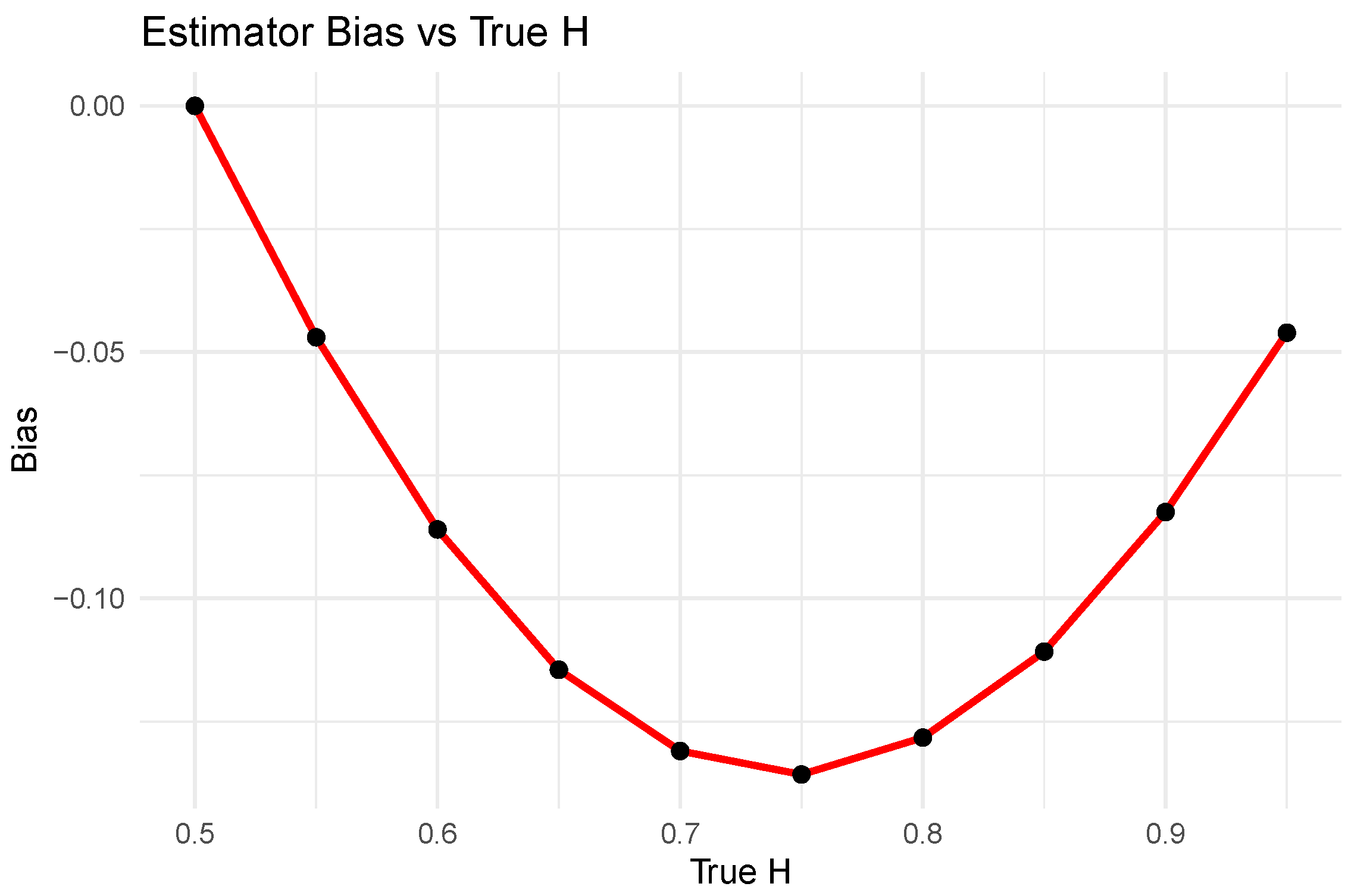
Figure 2 displays the bias of the MOM estimator as a function of the true Hurst parameter. The bias is zero at $H=0.5$ and becomes increasingly negative as H increases, reaching a minimum around $H=0.75$. This supports earlier results that the MOM estimator tends to underestimate the true Hurst parameter at higher values.

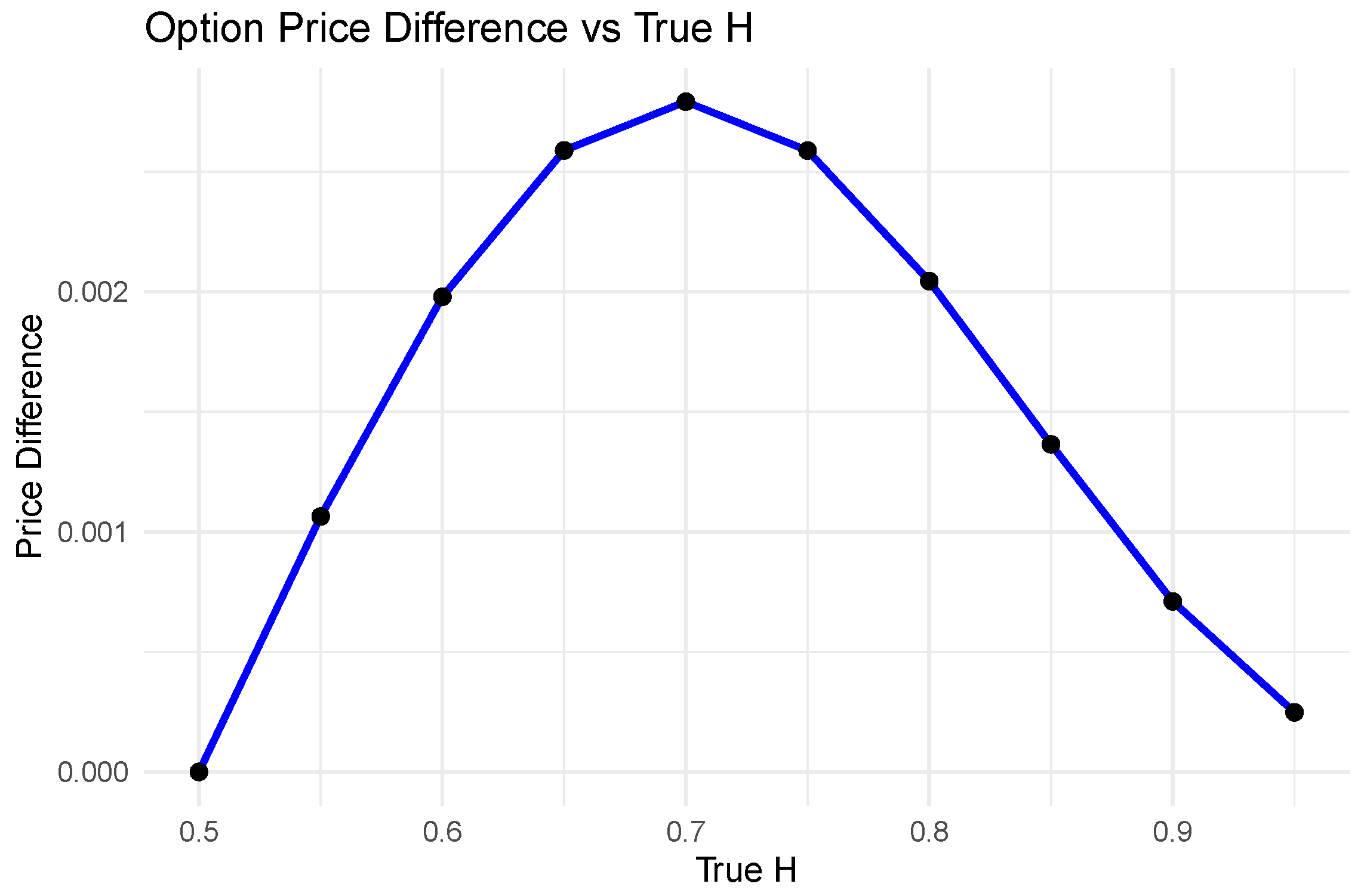
Figure 3 presents the absolute difference in option prices between two versions of the fractional Black–Scholes model: one using the true Hurst parameter, and the other using the MOM-estimated ${\widehat{H}}_{\mathrm{MOM}}$. Despite the estimator bias, the pricing error remains relatively small, peaking at around 0.0028 when $H\approx 0.7$. These results demonstrate that although the MOM estimator introduces bias in H, the impact on option pricing under the fBSM framework is modest. The fractional model appears moderately robust to such estimation error, particularly in moderate to high volatility regimes. This finding motivates continued use of corrected estimators in practical pricing scenarios, which we further refine in the next section.

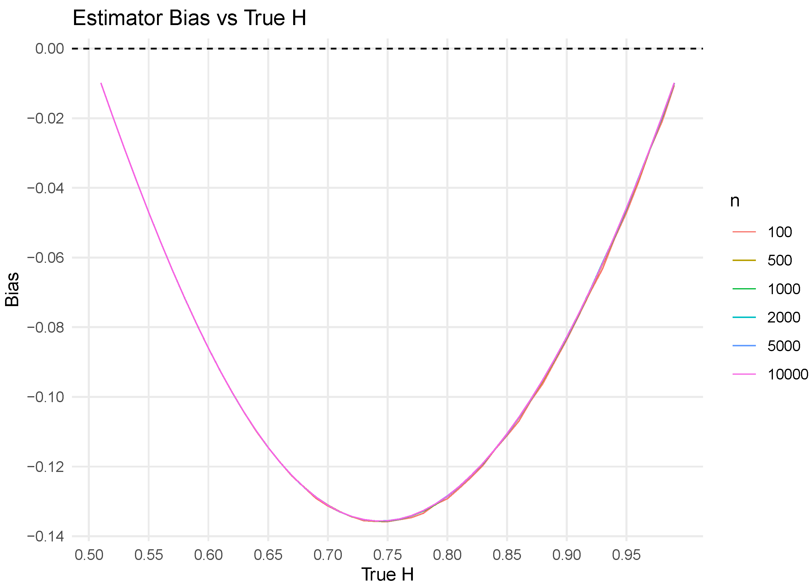
To examine how bias varies with sample size, we ran a simulation study with replications for each $H\in \{0.51,0.52,\dots ,0.99\}$ (step 0.01) and sample sizes n = 100, 250, 500, 1000, 5000, and 10,000. For each design point, we estimated $\widehat{H}$ using the MOM estimator and averaged the bias. Figure 4 shows that the bias curve is virtually unchanged across n, with the largest negative bias near $H\approx 0.72$. This indicates that a single, n-agnostic quadratic correction is adequate; the correction need not depend on sample size. The smooth, nearly monotone shape of the bias curve—with a single trough—also suggests that a low-degree polynomial can capture its structure. We therefore adopt a quadratic correction.

3.3. Bias Correction for the MOM Estimator

To model the estimation bias as a function of the true Hurst parameter H, we fitted a second-degree polynomial regression using simulation data over the interval $H\in \{0.50,0.55,\dots ,0.95\}$. For each value of H, 1000 fBM paths were simulated, and the bias was computed as the average ${\widehat{H}}_{\mathrm{MOM}}-H$. The fitted model is

$$\widehat{\mathrm{Bias}}\left(H\right)=a_0+a_{1}H+a_2{H}^2,$$

with coefficients:

$$a_0=1.09990,a_1=-3.30213,a_2=2.20769.$$

This regression explains over 99.9% of the variance in the observed bias (adjusted $R^2=0.9992$) with a residual standard error of 0.00125. The corrected estimate of the Hurst parameter is then given by

$${\widehat{H}}_{\mathrm{corr}}={\widehat{H}}_{\mathrm{MOM}}-\widehat{\mathrm{Bias}}\left({\widehat{H}}_{\mathrm{MOM}}\right),$$

where we substitute $H={\widehat{H}}_{\mathrm{MOM}}$ into the bias model. For example, if ${\widehat{H}}_{\mathrm{MOM}}=0.70$, the estimated bias is

$$\begin{array}{cc}\hfill \widehat{\mathrm{Bias}}\left(0.70\right)& =1.09990-3.30213\left(0.70\right)+2.20769{\left(0.70\right)}^2\hfill \end{array}$$

(1)

$$\begin{array}{cc}\hfill & =1.09990-2.31149+1.08577\hfill \end{array}$$

(2)

$$\begin{array}{cc}\hfill & =-0.12582.\hfill \end{array}$$

(3)

Thus, the corrected estimate becomes

$${\widehat{H}}_{\mathrm{corr}}=0.70-(-0.12582)=0.82582.$$

To ensure the corrected value remains within the theoretical range $(0.5,1)$, we apply truncation:

$${\widehat{H}}_{\mathrm{final}}=min\left(1,max\left(0.5,{\widehat{H}}_{\mathrm{corr}}\right)\right).$$

This correction significantly improves the alignment between estimated and true Hurst values, especially when $H>0.6$, where the MOM estimator shows the greatest deviation. This bias correction differs from prior work (Pramanik et al., 2024), which fixes the correction at 0 when $H=\frac{1}{2}$ and $H=1$. Our method does not impose these constraints and permits the data-driven correction needed to offset bias.

3.4. Improved Estimation of H

Figure 5 shows a comparison between the original and bias-corrected MOM estimates of the Hurst parameter. The corrected estimates (blue triangles) lie substantially closer to the identity line $\widehat{H}=H$ compared to the original MOM estimates (red circles), indicating that the bias correction improves accuracy. However, the corrected estimates still deviate slightly from the identity line, particularly at higher values of H, suggesting that some residual bias remains even after correction. This implies that the second-degree polynomial bias correction reduces, but does not fully eliminate, the systematic underestimation by the MOM estimator.

3.5. Impact on Option Pricing via the Fractional Black–Scholes Model

European call option prices under the fractional Black–Scholes model are computed using the closed-form expression derived in (Comte & Renault, 1998), which extends the classical Black–Scholes formula to the fBM-driven setting. To assess the effect of estimating H, we compute European call option prices under four configurations:

• The classical Black–Scholes model with $H=0.5$;
• The fractional Black–Scholes model using the true H;
• The fBSM using the uncorrected MOM estimate ${\widehat{H}}_{\mathrm{MOM}}$;
• The fBSM using the bias-corrected estimate ${\widehat{H}}_{\mathrm{final}}$.

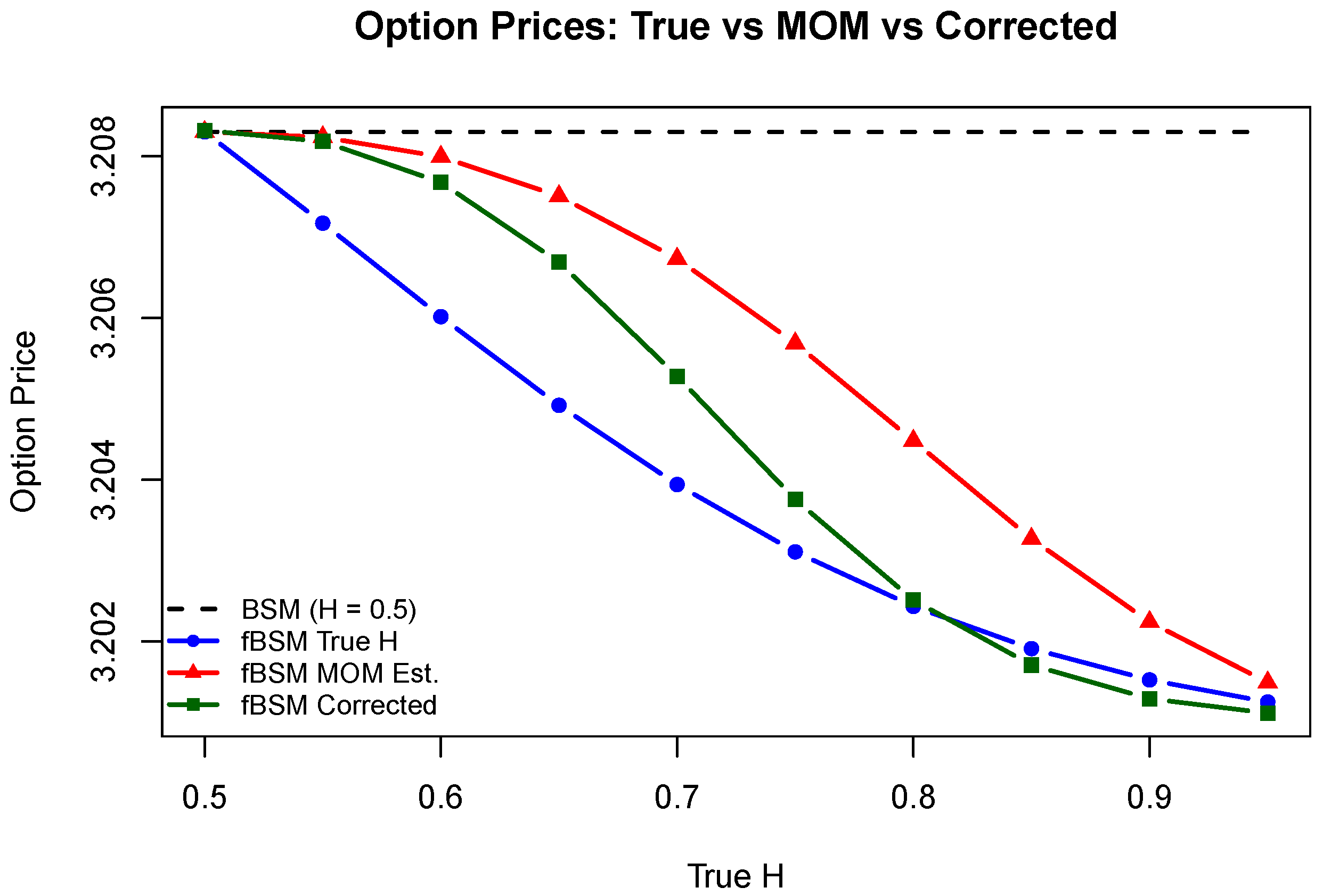
Figure 6 presents the resulting option prices across the different models. The fractional models yield prices that differ from the classical Black–Scholes baseline, especially when H is far from 0.5. Notably, the corrected estimator produces prices more consistent with those derived from the true H, whereas the uncorrected MOM estimator introduces larger pricing errors.

These results highlight the sensitivity of option prices to the value of H, reinforcing the importance of accurate estimation when applying fBSM models. In particular, the bias correction improves both the Hurst parameter estimates and the resulting price accuracy, supporting its use in financial applications.

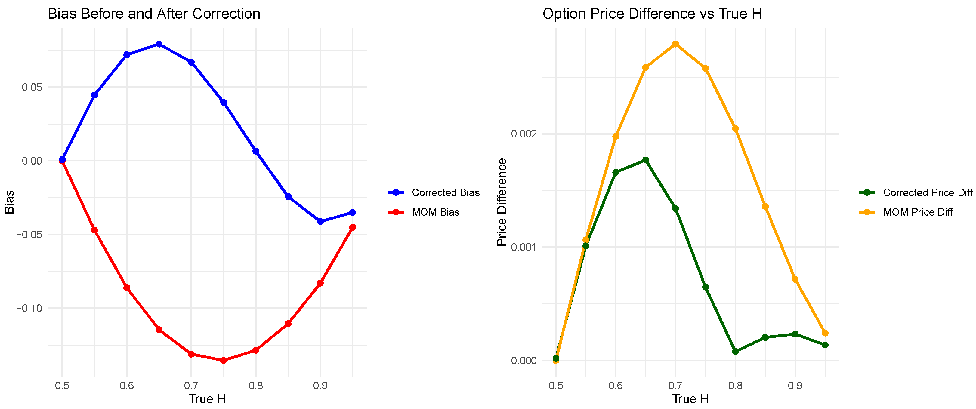
To quantify the improvement offered by the bias correction, Figure 7 presents two side-by-side plots: the left panel compares the bias before and after correction, and the right panel shows the absolute option price differences underestimated versus true H. Both panels show clear improvement after correction. In the left panel, the corrected estimator shows a substantial reduction in bias across all values of H, bringing the estimates closer to the true values. The right panel demonstrates that this reduction in bias also leads to lower pricing errors—especially in the region $H\in [0.65,0.8]$, where the original MOM bias was most pronounced. Overall, these results confirm that the proposed bias correction not only improves the statistical properties of the estimator but also enhances the practical accuracy of option pricing under the fractional Black–Scholes framework.

To quantitatively evaluate the performance improvements introduced by the bias correction strategy, we compute the root mean square error (RMSE) for both the Hurst parameter estimation and the resulting European call option prices.

Table 2. Root mean square error (RMSE) comparison for Hurst parameter estimation and corresponding option prices using MOM and bias-corrected MOM estimators.

Estimator	RMSE (H)	RMSE (Option Price)
MOM	0.0980	0.0018
Bias-Corrected MOM	0.0480	0.0010

presents the RMSE values for the MOM estimator and the bias-corrected estimator, averaged over 10 true H values in the range $[0.5,0.95]$.

As shown in Table 2, the bias correction nearly halves the RMSE in estimating the Hurst parameter and substantially reduces the RMSE in option pricing. This confirms that the bias correction improves both the statistical accuracy of H estimation and its financial implications in pricing, while adding negligible computational overhead.

4. Application to Real Financial Assets

Fractional models have been applied to option pricing in several contexts (Biagini et al., 2008; Comte et al., 2012; Mandelbrot, 1997). To demonstrate the practical implications of Hurst parameter estimation on option pricing, we apply our methodology to four representative financial assets: Natural Gas Futures, Apple Inc. (AAPL), Gold Futures, and Crude Oil Futures. These assets were chosen to cover a spectrum of volatility regimes and market characteristics, ranging from highly volatile energy commodities to more stable equity and precious metal series.

For each asset, daily adjusted closing prices are collected from Yahoo Finance. Let $P_t$ denote the adjusted closing price at time t. We compute daily log-returns as $r_t=\Delta log{P}_t=log\left(P_t\right)-log\left(P_{t-1}\right)$, from which annualized volatility is estimated based on a 252-trading-day convention. The Hurst parameter is then estimated using the Method of Moments (MOM), followed by application of our quadratic bias correction. These estimates are subsequently used to compute European call option prices under three frameworks: (i) the classical Black–Scholes model (BSM) with $H=0.5$, (ii) the fractional Black–Scholes model (fBSM) with ${\widehat{H}}_{\mathrm{MOM}}$, and (iii) the fBSM with the corrected ${\widehat{H}}_{\mathrm{final}}$.

The data spans the following timeframes:

• Natural Gas Futures (NG = F): 1 January 2022 to 31 October 2024;
• Apple Inc. (AAPL): 1 January 2023 to 31 December 2023;
• Gold Futures (GC = F): 1 January 2022 to 31 December 2024;
• Crude Oil Futures (CL = F): 1 January 2020 to 31 October 2024.

Table 3. Descriptive statistics of daily log-returns ($r_t=\Delta log{P}_t$).

Asset	n	Mean	Std. Dev.	Skewness	Kurtosis	Min	Max
Natural Gas (NG = F)	711	−0.00041	0.05240	0.26	8.93	−0.300	0.382
Apple (AAPL)	249	0.00175	0.01255	−0.05	4.42	−0.049	0.046
Gold (GC = F)	751	0.00049	0.00919	−0.26	3.94	−0.035	0.031
Crude Oil (CL = F)	1214	0.00009	0.03829	−3.14	66.94	−0.602	0.320

reports descriptive statistics (sample size n, mean, standard deviation, skewness, kurtosis, minimum, and maximum) of daily log-returns for each asset. These raw features contextualize the model-based volatility and Hurst estimates presented later. We remove days with missing adjusted closes; n counts valid daily returns after differencing.

The option pricing parameters are fixed across all assets: initial stock price $S_0=100$, strike price $K=98$, risk-free rate $r=0.05$, and time to maturity $T=90/365$ years. These fixed parameters provide a stylized benchmark that isolates the role of $\widehat{H}$ in option pricing. By holding $(S_0,K,r,T)$ constant, we ensure that observed pricing differences stem directly from long-memory effects rather than heterogeneity in contract specifications. In practice, strike prices and maturities vary by asset and market conditions; extending the analysis to market-specific contracts is a natural next step.

Table 4. Volatility, Hurst parameter estimates, and option prices under BSM and fBSM models.

Asset	Volatility	${\widehat{\mathit{H}}}_{\mathbf{MOM}}$	${\widehat{\mathit{H}}}_{\mathbf{final}}$	BSM Price	fBSM (MOM)	fBSM (Corrected)
Natural Gas	0.8318	0.5566	0.6107	17.7497	17.3490	16.9020
Apple	0.1992	0.5002	0.4997	5.6901	5.6898	5.6905
Gold	0.1459	0.5001	0.4994	4.7263	4.7262	4.7268
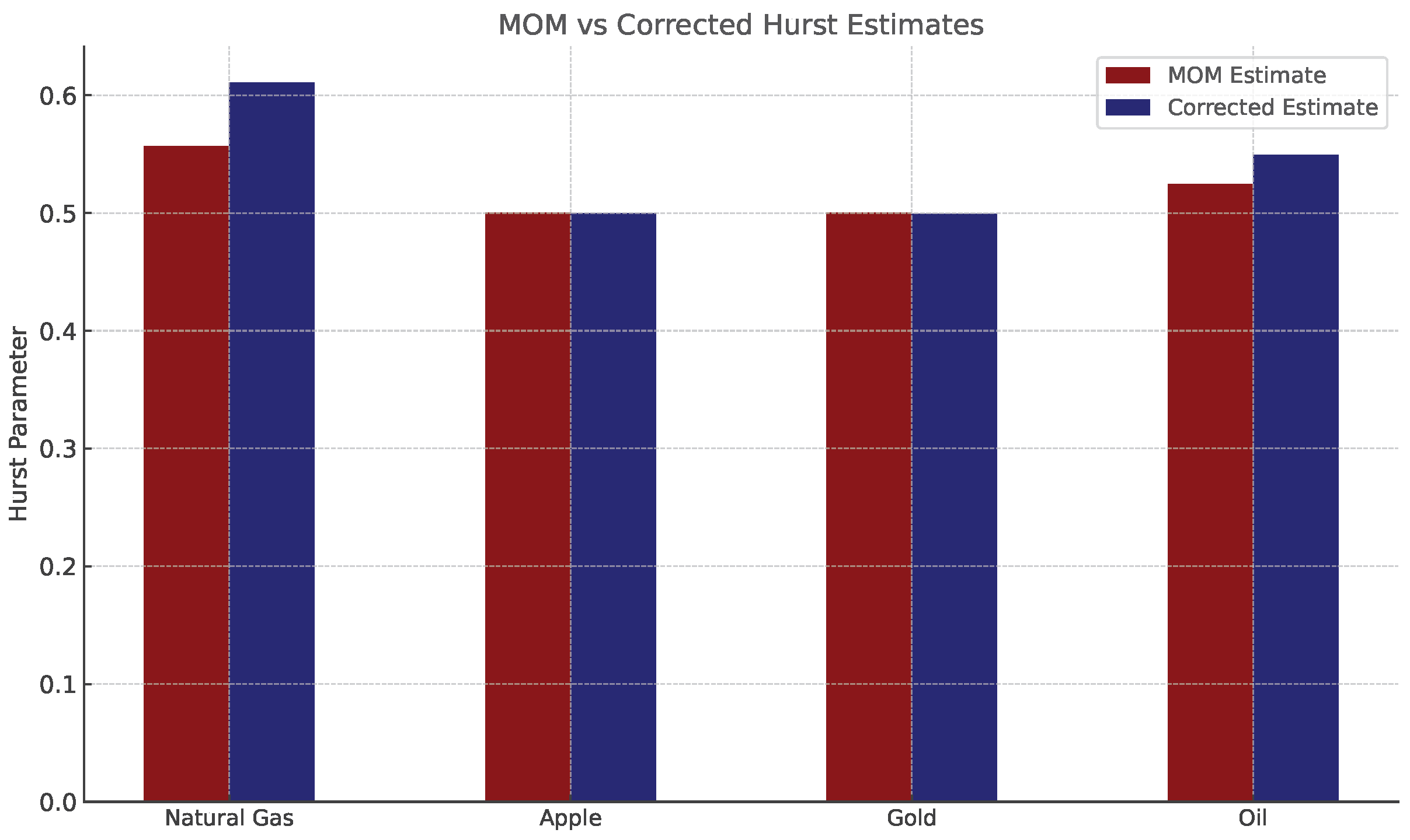
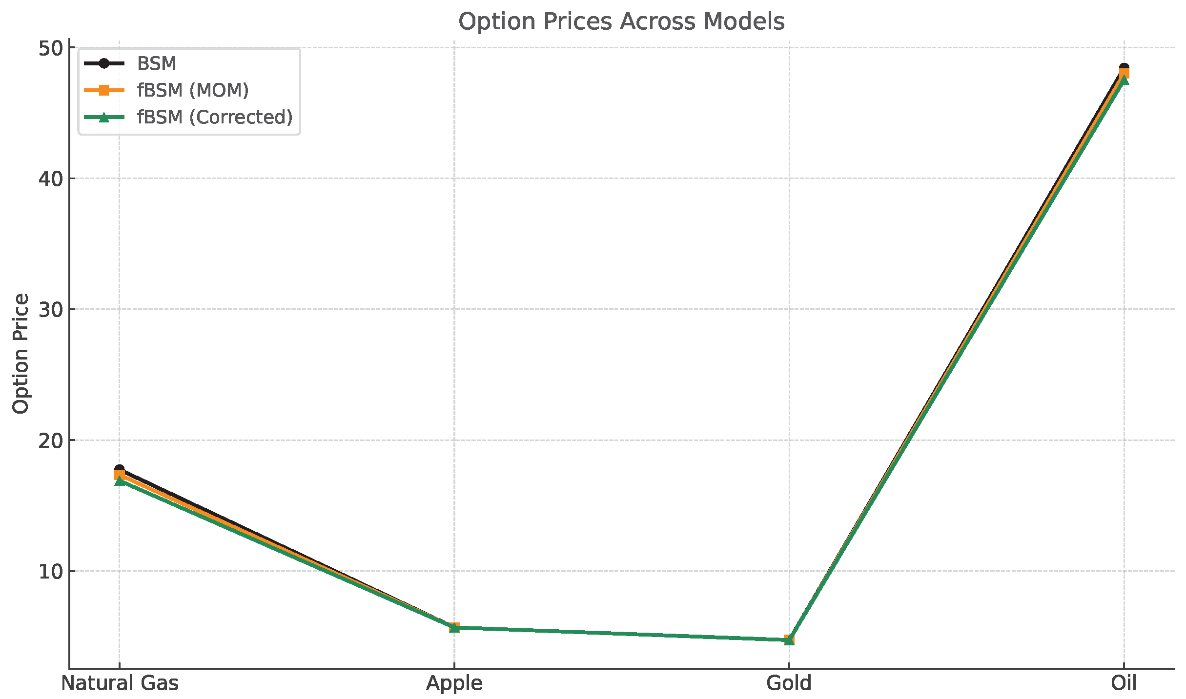
Oil	2.5648	0.5245	0.5492	48.4258	48.0039	47.5354

summarizes the estimated volatility, MOM, and corrected Hurst values, and the resulting option prices under the three modeling frameworks.

As a robustness check, we also compare our stylized benchmark with a realistic option contract for Apple Inc. (AAPL). On 29 December 2023, AAPL closed at approximately USD 192.5. Consider a European call option with strike price $K=190$ and time to maturity of three months (March 2024). Using the observed volatility $\sigma =0.1992$ and risk-free rate $r=0.05$, the classical Black–Scholes model yields a call price of about USD 7.85. Applying the fractional Black–Scholes model with ${\widehat{H}}_{\mathrm{MOM}}=0.5002$ and corrected ${\widehat{H}}_{\mathrm{final}}=0.4997$ produces nearly identical prices of USD 7.84 and USD7.85, respectively. This example confirms that for low-volatility, near-random-walk assets such as AAPL, bias in H estimation has minimal impact on option pricing, consistent with our benchmark findings.

As shown in Table 4, volatility varies widely across assets, with Crude Oil and Natural Gas exhibiting much higher volatility than Gold and Apple. Relative to the classical Black–Scholes model (BSM) with $H=0.5$, the fractional Black–Scholes model (fBSM) using the Method of Moments estimate ${\widehat{H}}_{\mathrm{MOM}}$ already produces noticeable deviations in option prices, particularly for the more volatile assets. This demonstrates the sensitivity of derivative pricing to long-memory effects when H departs from the random-walk case. Comparing fBSM (MOM) to fBSM (Corrected) further shows the role of bias correction: for Natural Gas and Oil, corrected estimates of H lower option prices by 0.4–0.5 units, highlighting the financial importance of mitigating estimator bias. By contrast, for Apple and Gold, which display relatively low volatility and Hurst values close to $0.5$, all three models—BSM, fBSM (MOM), and fBSM (Corrected)—yield nearly identical prices. This validates the intuition that near-random-walk assets are robust to bias in H estimation, while highly volatile, long-memory assets are much more sensitive to estimation accuracy.

Figure 8, Figure 9 and Figure 10 summarize these effects. Figure 8 compares MOM vs. corrected Hurst estimates, Figure 9 shows their impact on option prices, and Figure 10 illustrates implications for financial decision-making.

In sum, bias correction improves the reliability of Hurst parameter estimation, reduces option pricing error, and provides practitioners with a more robust framework for trading and hedging in long-memory markets. For Apple and Gold, corrections yield minimal changes, whereas for Natural Gas and Oil, pricing gaps of 0.4–0.5 units (equivalent to USD 40–USD 50 per contract under standard multipliers) highlight the tangible financial significance of accurate Hurst parameter estimation in volatile markets.

5. Discussion

Accurate estimation of the Hurst parameter H is critical when applying fractional models to financial time series, particularly in derivative pricing and risk management. While the Method of Moments (MOM) offers a computationally efficient closed-form estimator, our analysis confirms that it exhibits increasing negative bias as the true Hurst parameter deviates from 0.5, the range most relevant to long-memory processes in finance. If uncorrected, this bias propagates into systematic mispricing under the fractional Black–Scholes model (fBSM).

The proposed bias-corrected MOM estimator provides a practical solution to this challenge. It retains the computational simplicity of MOM while substantially reducing estimation error, as demonstrated through both simulation and real-data applications. Importantly, the correction improves pricing accuracy in volatile, long-memory markets such as energy commodities, where small parameter biases can translate into meaningful monetary consequences. By contrast, for relatively stable assets with low volatility and Hurst estimates near 0.5, the corrected and uncorrected models yield nearly identical prices, validating the robustness of such markets to estimator bias.

We emphasize that our focus is on improving the classical MOM estimator in contexts where closed-form simplicity and real-time implementability are essential. We deliberately do not benchmark against alternative estimators such as wavelet-based, log-periodogram, or Bayesian methods, as the contribution here is to enhance MOM’s accuracy without sacrificing efficiency. In related parametric formulations, the MOM estimator coincides with the MLE; however, prior bias corrections enforce boundary constraints at $H=\frac{1}{2}$ and $H=1$, whereas our correction is unconstrained on $H\in (0,1)$ (Pramanik et al., 2024). A natural next step is a distributed version of the bias-corrected MOM for very long or high-frequency series: partition the data into (possibly overlapping) blocks, estimate H locally, and then use a COR-style optimal subset-selection stage to retain the most informative blocks before aggregation, yielding a communication-efficient pipeline with improved stability and inference (Chen & Xie, 2014; G. Guo et al., 2024; Jordan et al., 2019).

These findings confirm that bias correction is not merely a statistical refinement but a financially significant adjustment in derivative pricing. Prior studies have highlighted the importance of long memory in financial modeling (e.g., Comte & Renault, 1998; Gatheral et al., 2018; Mandelbrot, 1997), yet few have directly addressed the systematic bias of standard estimators. By introducing and validating a bias-corrected MOM framework, this work narrows the gap between theoretical efficiency and practical accuracy in long-memory option pricing. Future research may extend the approach to benchmark comparisons, alternative estimation frameworks, and broader classes of derivatives to further explore the trade-off between simplicity and precision in fractional financial modeling.

6. Conclusions

This paper introduced a bias-corrected Method of Moments (MOM) estimator for the Hurst parameter H, offering a closed-form and computationally efficient approach that substantially reduces the bias of the classical MOM. Simulation experiments and empirical applications confirmed that the corrected estimator improves both parameter accuracy and option pricing under the fractional Black–Scholes model.

Beyond European call options, the corrected estimator has potential for other derivatives sensitive to long-memory effects, such as barrier and Asian options, and for high-frequency or streaming estimation settings. Future work could extend this framework by benchmarking against alternative estimators, exploring integration with Bayesian or maximum likelihood methods, and assessing robustness under model misspecification (e.g., jump diffusion or regime-switching). Finally, evaluating the economic value of improved H estimation in portfolio management, hedging strategies, and algorithmic trading would provide further insight into its practical impact.