Bitcoin Supply, Demand, and Price Dynamics
Abstract
1. Introduction
2. Background
2.1. Bitcoin’s Fixed Supply
2.2. Liquid Supply
2.3. Market Demand
2.4. Market Outflows
3. Methodology
3.1. Previous Bitcoin Supply-and-Demand Model
3.2. Modeling Context
3.3. Model Structure
3.3.1. Supply
3.3.2. Demand Function
3.3.3. Withdrawals from Liquid Supply
3.4. Baseline Model: Calibration
- The logistic adoption curve parameters were initially fixed at T* = 14 years and L_min = 0.05, giving a relatively slow rate of growth over the model’s time horizon, not reaching the saturation point until two years after the framework’s April 2036 (7th halving) time horizon.
- The demand multiplier was restricted to a choice of D = [10, 20, 30] because higher multiples seemed implausible over 2024–2025.
- The EZ parameter ρ was set to 2.0, a value that suggests the majority of allocators have relatively low time preferences. Given the continual flows into illiquid supply and the ancient 5+ year cohort, this seems consistent with market conditions since the 2024 halving.
- Baseline withdrawals, qbase, were limited to seemingly plausible 2024–2025 values of qbase = [1000, 2000, 3000].
- The withdrawal-sensitivity parameter, α, was set to 0.10, providing a modest reduction in daily Bitcoin purchase volume as price appreciates (11× price appreciation leads to 50% reduction in purchases).
3.5. Baseline Model: Exploration of Parameterization Impacts
3.5.1. Demand Multiplier
3.5.2. Epstein–Zin Intertemporal Substitution Parameter
3.5.3. Withdrawal Options
3.5.4. Withdrawal Sensitivity
3.5.5. Two-Way Interactions
3.6. Compound Annual Growth Rate
3.7. Monte Carlo Simulation with Uniform Parameter Distributions
4. Results
4.1. Baseline Model
4.2. Variations on the Baseline Model
4.2.1. Changes in the Demand-Shift Parameter
4.2.2. Changes in the Epstein–Zin Intertemporal Substitution
4.2.3. Changes in the Daily Withdrawals from Liquid Supply
4.2.4. Changes in the Withdrawal-Sensitivity Parameter
4.3. Combined Supply Parameter Changes
4.3.1. Changes in the Withdrawal-Sensitivity Parameter and Level of Withdrawal
4.3.2. Changes in the Withdrawal-Sensitivity and EIS Parameters
4.4. Monte Carlo Simulation
4.4.1. Price Forecast Distribution
4.4.2. Implications of Shifting Liquidity Assumptions
4.4.3. Exceedance Probabilities
5. Discussion
5.1. Growth in Demand
5.2. Comparison with Existing Financial Models
5.3. Liquid Supply and Execution Discipline
5.4. Hyperbolic Price Trajectories
5.5. Limitations and Future Research
6. Conclusions
Supplementary Materials
Author Contributions
Funding
Institutional Review Board Statement
Informed Consent Statement
Data Availability Statement
Conflicts of Interest
References
- Ang, A., Morris, T., & Savi, R. (2022). Asset allocation with crypto: Application of preferences for positive skewness. The Journal of Alternative Investments, 25, 7–28. [Google Scholar] [CrossRef]
- Arrow, K. J., Chenery, H. B., Minhas, B. S., & Solow, R. M. (1961). Capital-labor substitution and economic efficiency. The Review of Economics and Statistics 43, 225–250. [Google Scholar] [CrossRef]
- Augustin, P., Rubtsov, A., & Shin, D. (2023). The impact of derivatives on spot markets: Evidence from the introduction of Bitcoin futures contracts. Management Science, 69, 6752–6776. [Google Scholar] [CrossRef]
- Biais, B., Bisière, C., Bouvard, M., Casamatta, C., & Menkveld, A. J. (2023). Equilibrium Bitcoin pricing. The Journal of Finance, 78, 967–1014. [Google Scholar] [CrossRef]
- Bordo, M., Monnet, E., & Naef, A. (2019). The gold pool (1961–1968) and the fall of the bretton woods system: Lessons for central bank cooperation. The Journal of Economic History, 79, 1027–1059. [Google Scholar] [CrossRef]
- Ciaian, P., Rajcaniova, M., & Kancs, D. (2016). The economics of BitCoin price formation. Applied Economics, 48, 1799–1815. [Google Scholar] [CrossRef]
- Dyhrberg, A. H. (2016). Hedging capabilities of bitcoin. Is it the virtual gold? Finance Research Letters, 16, 139–144. [Google Scholar] [CrossRef]
- Epoch Management. (2025). The Bitcoin ecosystem: 2024 annual report. Available online: https://epochvc.io/pdf/Epoch-Bitcoin-Ecosystem-Report-2024.pdf (accessed on 21 August 2025).
- Epstein, L. G., & Zin, S. E. (1991). Substitution, risk aversion, and the temporal behavior of consumption and asset returns: An empirical analysis. Journal of Political Economy, 99, 263–286. [Google Scholar] [CrossRef]
- Feder-Sempach, E., Szczepocki, P., & Bogołębska, J. (2024). Global uncertainty and potential shelters: Gold, bitcoin, and currencies as weak and strong safe havens for main world stock markets. Financial Innovation, 10, 67. [Google Scholar] [CrossRef]
- Jacks, D. S. (2019). From boom to bust: A typology of real commodity prices in the long run. Cliometrica, 13, 201–220. [Google Scholar] [CrossRef]
- Ji, S., Kim, J., & Im, H. (2019). A comparative study of bitcoin price prediction using deep learning. Mathematics, 7, 898. [Google Scholar] [CrossRef]
- Kearney, J. J., & Perez-Delgado, C. A. (2021). Vulnerability of blockchain technologies to quantum attacks. Array, 10, 100065. [Google Scholar] [CrossRef]
- Mazur, M., & Polyzos, E. (2025). Spot Bitcoin ETFs: The effect of fund flows on Bitcoin price formation. The Journal of Alternative Investments, 27, 110–123. [Google Scholar] [CrossRef]
- Mehra, R., & Prescott, E. C. (1985). The equity premium: A puzzle. Journal of Monetary Economics, 15, 145–161. [Google Scholar] [CrossRef]
- Mejri, S., Leccadito, A., & Yildirim, R. (in press). Dynamic responses of Bitcoin, gold, and green bonds to geopolitical risk: A quantile wavelet analysis. Borsa Istanbul Review. [CrossRef]
- Mohamad, A. (2025). Do Bitcoin ETFs lead price discovery following their introduction in the Bitcoin market? Computational Economics, 66, 947–969. [Google Scholar] [CrossRef]
- Nabben, K. (2023). Cryptoeconomics as governance: An intellectual history from “Crypto Anarchy” to “Cryptoeconomics”. Internet Histories, 7(3), 254–276. [Google Scholar] [CrossRef]
- Nakamoto, S. (2008). Bitcoin: A peer-to-peer electronic cash system. Unpublished white paper. Available online: https://bitcoin.org/bitcoin.pdf (accessed on 21 August 2025).
- Narayanan, A., & Clark, J. (2017). Bitcoin’s academic pedigree. Communications of the ACM, 60, 36–45. [Google Scholar] [CrossRef]
- National Economic Council. (2025). Strengthening American leadership in digital financial technology. The President’s Working Group on Digital Asset Markets. Available online: https://www.whitehouse.gov/crypto/ (accessed on 21 August 2025).
- River Financial. (2022). What could Bitcoin mining look like at one zettahash? Available online: https://river.com/learn/files/river-bitcoin-mining-zettahash-report.pdf (accessed on 21 August 2025).
- Roberts, M. J., & Schlenker, W. (2013). Identifying supply and demand elasticities of agricultural commodities: Implications for the US ethanol mandate. American Economic Review, 103, 2265–2295. [Google Scholar] [CrossRef]
- Rudd, M. A. (2025). Bitcoin worlds. SSRN preprint. [CrossRef]
- Rudd, M. A., & Porter, D. (2025). A supply and demand framework for Bitcoin price forecasting. Journal of Risk and Financial Management, 18, 66. [Google Scholar] [CrossRef]
- SEC. (1982). The silver crisis of 1980. A report of the staff of the U.S. Securities and Exchange Commission (SEC). Available online: https://www.sechistorical.org/collection/papers/1980/1982_1001_SECSilverCrisis_01.pdf (accessed on 21 August 2025).
- Shiva Sankari, V., & Kavitha, R. (2025). Bitcoin adoption and price elasticity of demand: Cross-country insights. Humanities and Social Sciences Communications, 12, 930. [Google Scholar] [CrossRef]
- Sun, W., Jin, H., Jin, F., Kong, L., Peng, Y., & Dai, Z. (2022). Spatial analysis of global Bitcoin mining. Scientific Reports, 12, 10694. [Google Scholar] [CrossRef]
- van Huellen, S. (2020). Too much of a good thing? Speculative effects on commodity futures curves. Journal of Financial Markets, 47, 100480. [Google Scholar] [CrossRef]
- Wakker, P. P. (2008). Explaining the characteristics of the power (CRRA) utility family. Health Economics, 17, 1329–1344. [Google Scholar] [CrossRef] [PubMed]
- Wheatley, S., Sornette, D., Huber, T., Reppen, M., & Gantner, R. N. (2019). Are Bitcoin bubbles predictable? Combining a generalized Metcalfe’s Law and the Log-Periodic Power Law Singularity model. Royal Society Open Science, 6, 180538. [Google Scholar] [CrossRef] [PubMed]
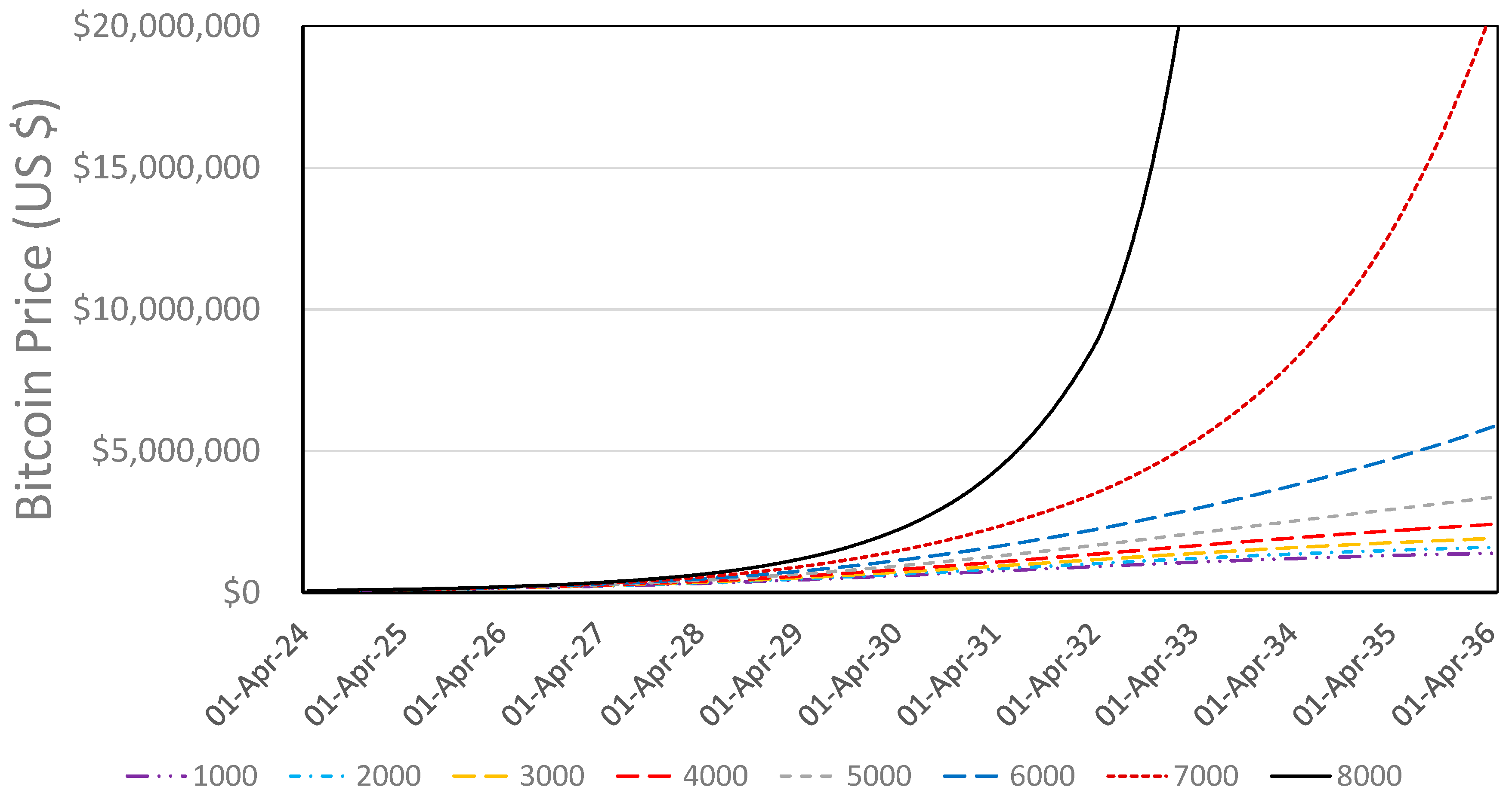
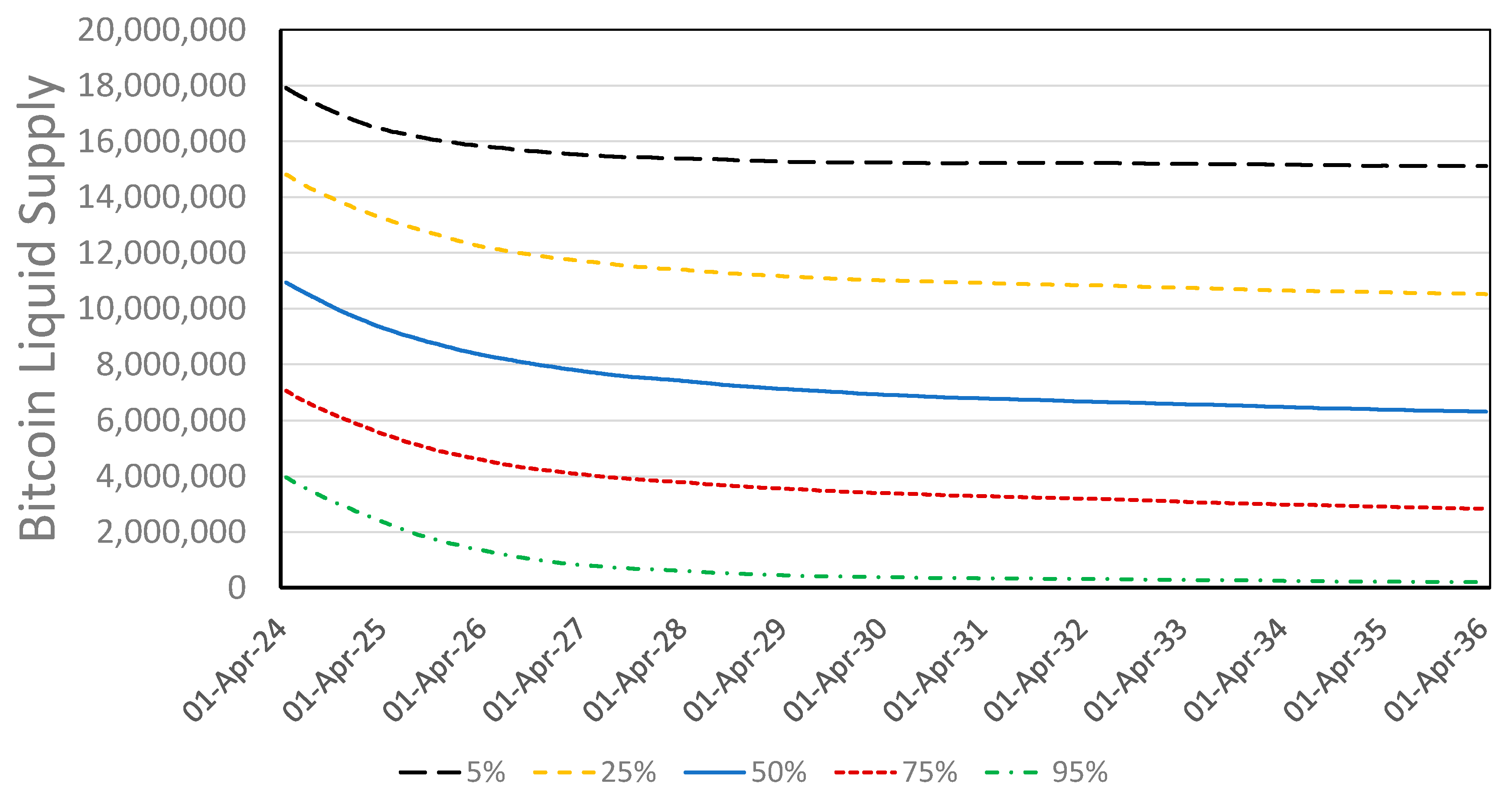
| # of Bitcoin | Value (Billion, USD) | % of Total Supply | |
|---|---|---|---|
| Total supply | 21,000,000 | USD 2476.1 | 100% |
| Remaining to be mined | 1,100,903 | USD 129.8 | 5.2% |
| Circulating supply | 19,899,097 | USD 2346.3 | 94.8% |
| Lost | |||
| Satoshi | 968,000 | USD 114.1 | 4.6% |
| Other | 1,570,000 | USD 185.1 | 7.5% |
| Effective circulating supply | 17,361,097 | USD 2047.1 | 82.7% |
| Institutions and governments | |||
| ETFs | 1,485,019 | USD 175.1 | 7.1% |
| Countries | 517,296 | USD 61.0 | 2.5% |
| Public companies | 900,868 | USD 106.2 | 4.3% |
| Private companies | 412,470 | USD 48.6 | 2.0% |
| Bitcoin mining companies | 107,858 | USD 12.7 | 0.5% |
| Locked in DeFi apps | 166,330 | USD 19.6 | 0.8% |
| Subtotal: Institutional | 3,589,841 | USD 423.3 | 17.1% |
| Individual/unknown holders | 13,771,256 | USD 1623.8 | 65.6% |
| Scenario | L_min | T* (Years) | D | qbase | Forecast Price, 21 April 2024 | Forecast Price, 29 July 2025 |
|---|---|---|---|---|---|---|
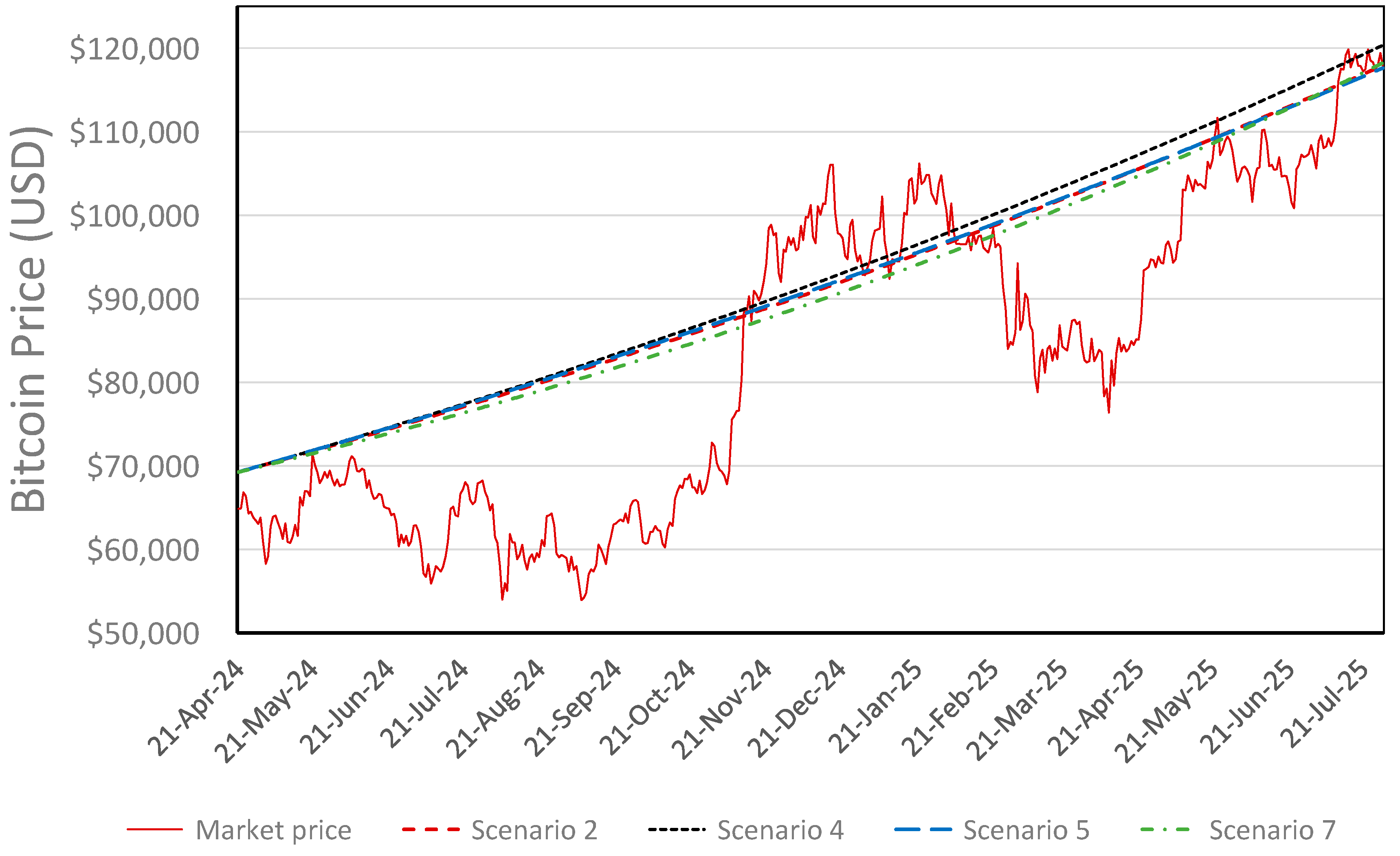
| 1 | 0.02 | 6 | 10 | 1000 | USD 69,229 | USD 119,932 |
| 2 | 0.05 | 14 | 20 | 1000 | USD 69,264 | USD 117,917 |
| 3 | 0.08 | 10 | 10 | 3000 | USD 69,257 | USD 119,296 |
| 4 * | 0.05 | 14 | 20 | 2000 | USD 69,264 | USD 120,340 |
| 5 | 0.06 | 16 | 20 | 2000 | USD 69,263 | USD 117,609 |
| 6 | 0.02 | 10 | 20 | 3000 | USD 69,241 | USD 119,274 |
| 7 | 0.03 | 12 | 20 | 3000 | USD 69,249 | USD 118,227 |
| 8 | 0.01 | 10 | 30 | 3000 | USD 69,235 | USD 119,382 |
| Scenario | L_min | T* (Years) | D | qbase | Price, 16 April 2036 | Market Cap, 16 April 2036 | Liquid Supply, 16 April 2036 | CAGR (12 Years) | Date for p = USD 1 M |
|---|---|---|---|---|---|---|---|---|---|
| 2 | 0.05 | 14 | 20 | 1000 | USD 1.39 | USD 29.0 T | USD 9.92 M | 29.1% | 15 October 2032 |
| 4 * | 0.06 | 16 | 20 | 2000 | USD 1.47 | USD 30.7 T | USD 7.22 M | 29.7% | 19 February 2033 |
| 5 | 0.03 | 12 | 20 | 3000 | USD 1.97 | USD 41.0 T | USD 5.82 M | 32.9% | 21 August 2030 |
| 7 | 0.05 | 14 | 20 | 2000 | USD 1.60 | USD 33.4 T | 7.48 M | 30.6% | 24 February 2032 |
| Variation | D | ρ | qbase | α | Price, 16 April 2036 | Market Cap, 16 April 2036 | Liquid Supply, 16 April 2036 | CAGR (12 Years) | Date for p = USD 1 M |
|---|---|---|---|---|---|---|---|---|---|
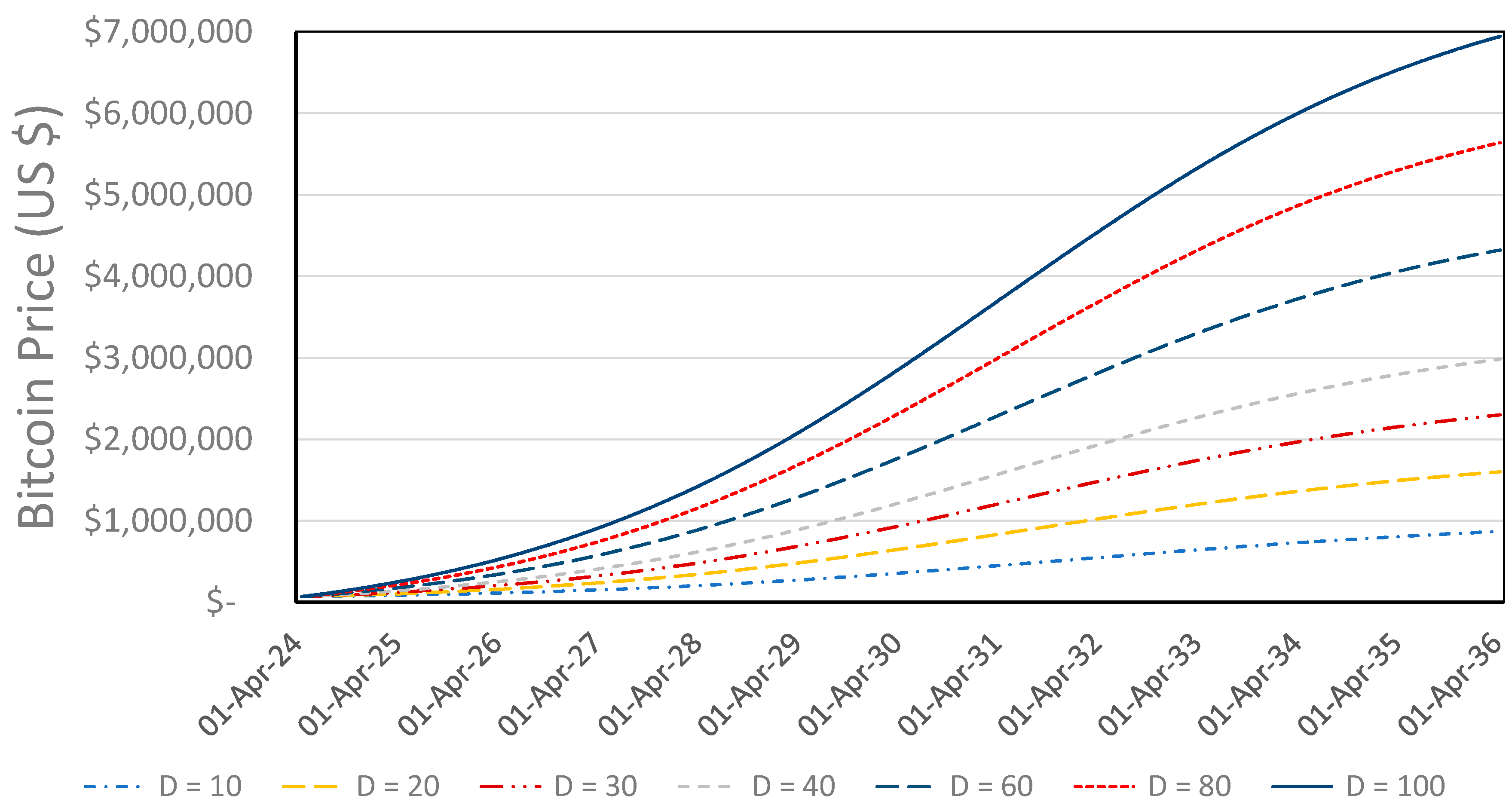
| 01 | 10 | 0.20 | 2000 | 0.10 | USD 0.87 M | USD 18.1 T | 6.38 M | 24.2% | n/a |
| 02 | 20 | 0.20 | 2000 | 0.10 | USD 1.60 M | USD 33.4 T | 7.48 M | 30.6% | 24 February 2032 |
| 03 | 30 | 0.20 | 2000 | 0.10 | USD 2.30 M | USD 47.9 T | 8.14 M | 34.7% | 9 July 2030 |
| 04 | 40 | 0.20 | 2000 | 0.10 | USD 2.98 M | USD 62.1 T | 8.59 M | 37.6% | 16 August 2029 |
| 05 | 60 | 0.20 | 2000 | 0.10 | USD 4.32 M | USD 90.0 T | 9.20 M | 41.9% | 27 July 2028 |
| 06 | 80 | 0.20 | 2000 | 0.10 | USD 5.64 M | USD 117.5 T | 9.60 M | 45.1% | 3 December 2027 |
| 07 | 100 | 0.20 | 2000 | 0.10 | USD 6.94 M | USD 144.6 T | 9.89 M | 47.6% | 20 June 2027 |
| Variation | D | ρ | qbase | α | Price, 16 April 2036 | Market Cap, 16 April 2036 | Liquid Supply, 16 April 2036 | CAGR (12 Years) | Date for p = USD 1 M |
|---|---|---|---|---|---|---|---|---|---|
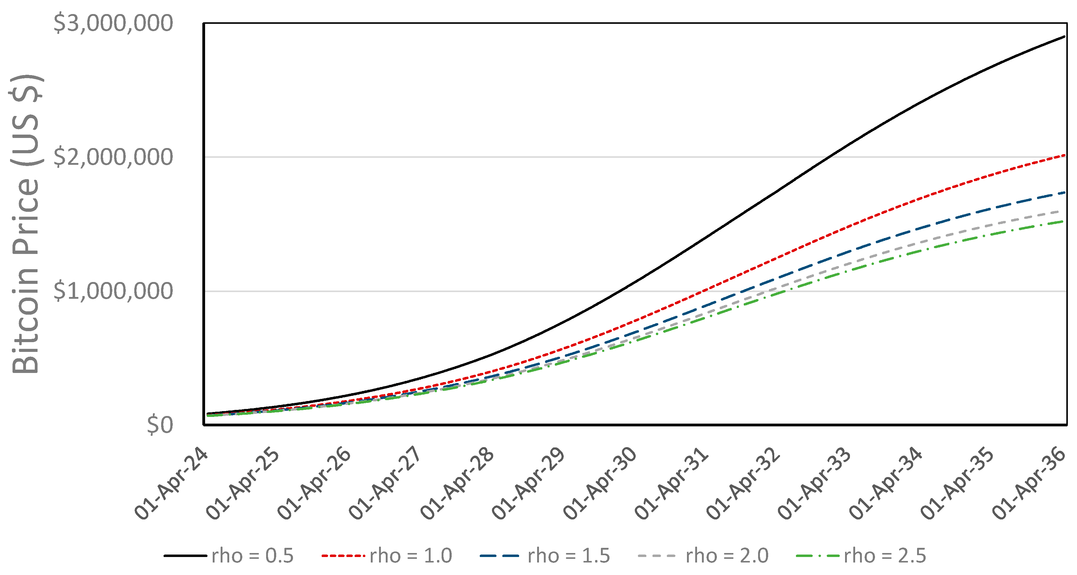
| 01 | 20 | 0.5 | 2000 | 0.10 | USD 2.90 M | USD 60.4 T | 8.39 M | 24.2% | 27 January 2030 |
| 02 | 20 | 1.0 | 2000 | 0.10 | USD 2.01 M | USD 41.2 T | 7.83 M | 30.6% | 29 March 2031 |
| 03 | 20 | 1.5 | 2000 | 0.10 | USD 1.74 M | USD 36.2 T | 7.60 M | 34.7% | 21 October 2031 |
| 04 | 20 | 2.0 | 2000 | 0.10 | USD 1.60 M | USD 33.4 T | 7.48 M | 30.7% | 24 February 2032 |
| 05 | 20 | 2.5 | 2000 | 0.10 | USD 1.52 M | USD 31.7 T | 7.41 M | 41.9% | 19 May 2032 |
| Variation | D | ρ | qbase | α | Price, 16 April 2036 | Market Cap, 16 April 2036 | Liquid Supply, 16 April 2036 | CAGR (12 Years) | Date for p = USD 1 M |
|---|---|---|---|---|---|---|---|---|---|
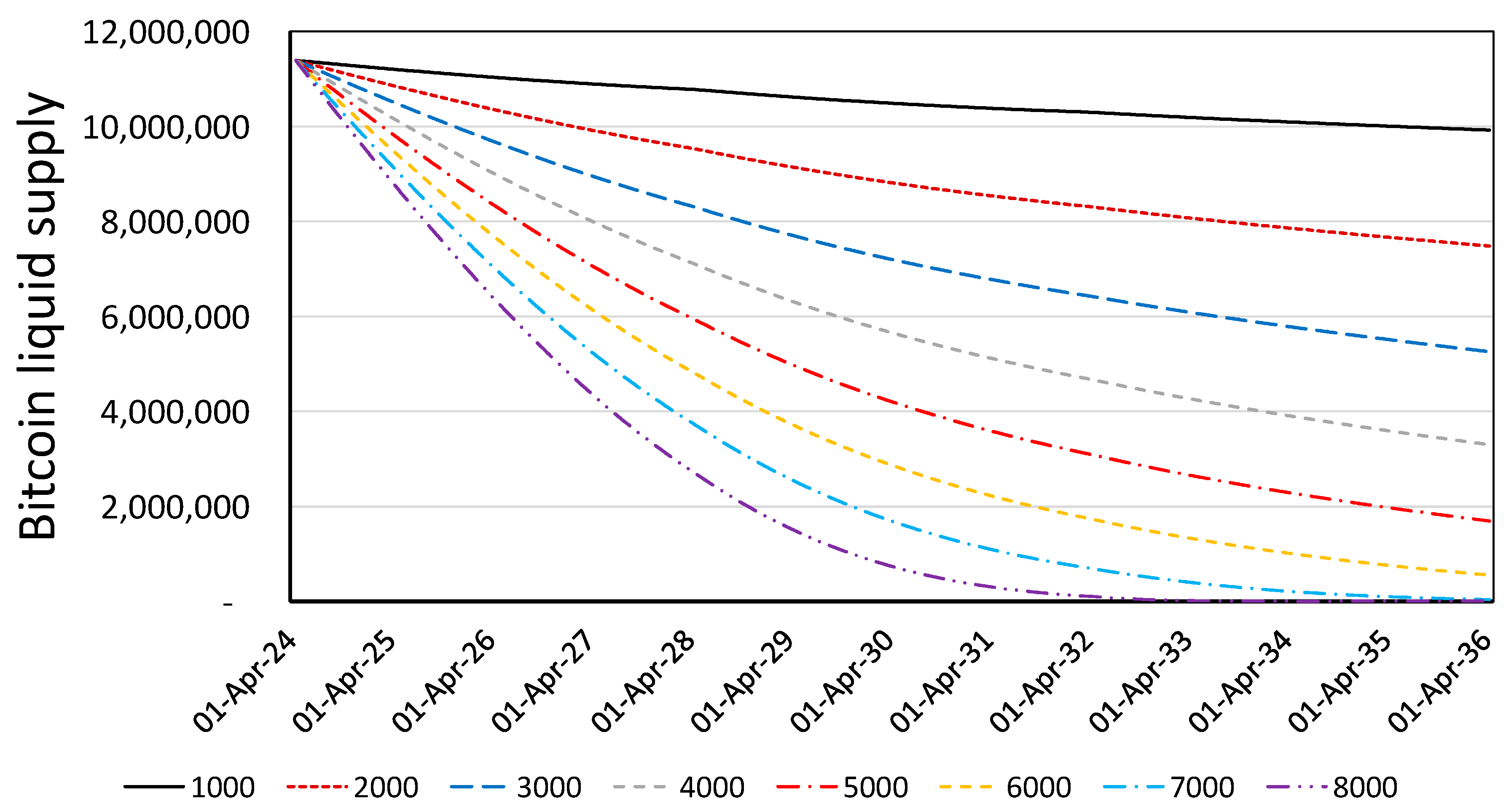
| 01 | 20 | 0.20 | 1000 | 0.10 | USD 1.39 M | USD 29.0 T | 9.92 M | 29.1% | 15 October 2032 |
| 02 | 20 | 0.20 | 2000 | 0.10 | USD 1.60 M | USD 33.4 T | 7.48 M | 30.6% | 24 February 2032 |
| 03 | 20 | 0.20 | 3000 | 0.10 | USD 1.91 M | USD 39.8 T | 5.26 M | 32.6% | 22 July 2031 |
| 04 | 20 | 0.20 | 4000 | 0.10 | USD 2.41 M | USD 50.2 T | 3.30 M | 35.17% | 30 December 2030 |
| 05 | 20 | 0.20 | 5000 | 0.10 | USD 3.36 M | USD 70.1 T | 1.70 M | 39.0% | 18 June 2030 |
| 06 | 20 | 0.20 | 6000 | 0.10 | USD 5.86 M | USD 122.1 T | 0.56 M | 45.6% | 13 December 2029 |
| 07 | 20 | 0.20 | 7000 | 0.10 | USD 20.69 M | USD 431.2 T | 0.04 M | 61.7% | 19 Jun 2029 |
| 08 | 20 | 0.20 | 8000 | 0.10 | USD 46.56 M | USD 970.2 T | <0.01 M | 73.0% | 3 January 2029 |
| Variation | D | ρ | qbase | α | Price, 16 April 2036 | Market Cap, 16 April 2036 | Liquid Supply, 16 April 2036 | CAGR (12 Years) | Date for p = USD 1 M |
|---|---|---|---|---|---|---|---|---|---|
| 01 | 20 | 0.20 | 2000 | 0.025 | USD 1.87 M | USD 38.9 T | 5.50 M | 32.3% | 30 October 2031 |
| 02 | 20 | 0.20 | 2000 | 0.050 | USD 1.73 M | USD 36.0 T | 6.42 M | 31.5% | 17 December 2031 |
| 03 | 20 | 0.20 | 2000 | 0.10 | USD 1.60 M | USD 33.4 T | 7.48 M | 30.6% | 24 February 2032 |
| 04 | 20 | 0.20 | 2000 | 0.20 | USD 1.49 M | USD 31.2 T | 8.58 M | 29.9% | 20 May 2032 |
| 05 | 20 | 0.20 | 2000 | 0.30 | USD 1.44 M | USD 30.1 T | 9.19 M | 29.6% | 12 July 2032 |
| 06 | 20 | 0.20 | 2000 | 0.40 | USD 1.41 M | USD 29.5 T | 9.60 M | 29.3% | 21 August 2032 |
| 07 | 20 | 0.20 | 2000 | 0.50 | USD 1.39 M | USD 29.0 T | 9.89 M | 29.1% | 17 September 2032 |
| Variation | D | ρ | qbase | α | Price, 16 April 2036 | Market Cap, 16 April 2036 | Liquid Supply, 16 April 2036 | CAGR (12 Years) | Date for p = USD 1 M |
|---|---|---|---|---|---|---|---|---|---|
| 01 | 20 | 0.20 | 2000 | 0.025 | USD 1.87 M | USD 38.9 T | 5.50 M | 32.3% | 30 October 2031 |
| 02 | 20 | 0.20 | 2000 | 0.050 | USD 1.73 M | USD 36.0 T | 6.42 M | 31.5% | 17 December 2031 |
| 03 | 20 | 0.20 | 2000 | 0.10 | USD 1.60 M | USD 33.4 T | 7.48 M | 30.6% | 24 February 2032 |
| 04 | 20 | 0.20 | 2000 | 0.20 | USD 1.49 M | USD 31.2 T | 8.58 M | 29.9% | 20 May 2032 |
| 05 | 20 | 0.20 | 2000 | 0.30 | USD 1.44 M | USD 30.1 T | 9.19 M | 29.6% | 12 July 2032 |
| 06 | 20 | 0.20 | 2000 | 0.40 | USD 1.41 M | USD 29.5 T | 9.60 M | 29.3% | 19 August 2032 |
| 07 | 20 | 0.20 | 2000 | 0.50 | USD 1.39 M | USD 29.0 T | 9.89 M | 29.1% | 17 September 2032 |
| 08 | 20 | 0.20 | 4000 | 0.025 | hyperbolic | hyperbolic | 0.22 M | n/a | 20 June 2030 |
| 09 | 20 | 0.20 | 4000 | 0.050 | USD 3.52 M | USD 73.4 T | 1.55 M | 39.6% | 5 September 2030 |
| 10 | 20 | 0.20 | 4000 | 0.10 | USD 2.41 M | USD 50.2 T | 3.30 M | 35.2% | 30 December 2030 |
| 11 | 20 | 0.20 | 4000 | 0.20 | USD 1.92 M | USD 40.0 T | 5.19 M | 32.7% | 30 May 2031 |
| 12 | 20 | 0.20 | 4000 | 0.30 | USD 1.75 M | USD 36.5 T | 6.26 M | 31.6% | 3 September 2031 |
| 13 | 20 | 0.20 | 4000 | 0.40 | USD 1.66 M | USD 34.5 T | 6.99 M | 31.0% | 11 November 2031 |
| 14 | 20 | 0.20 | 4000 | 0.50 | USD 1.60 M | USD 33.3 T | 7.52 M | 30.6% | 2 January 2032 |
| 15 | 20 | 0.20 | 8000 | 0.025 | hyperbolic | hyperbolic | <0.01 M | n/a | 3 May 2028 |
| 16 | 20 | 0.20 | 8000 | 0.050 | hyperbolic | hyperbolic | <0.01 M | n/a | 30 July 2028 |
| 17 | 20 | 0.20 | 8000 | 0.10 | hyperbolic | hyperbolic | <0.01 M | n/a | 3 January 2029 |
| 18 | 20 | 0.20 | 8000 | 0.20 | USD 5.17 M | USD 107.8 T | 0.72 M | 44.0% | 2 September 2029 |
| 19 | 20 | 0.20 | 8000 | 0.30 | USD 3.16 M | USD 65.8 T | 1.92 M | 38.3% | 18 February 2030 |
| 20 | 20 | 0.20 | 8000 | 0.40 | USD 2.57 M | USD 53.5 T | 2.91 M | 35.9% | 21 June 2030 |
| 21 | 20 | 0.20 | 8000 | 0.50 | USD 2.28 M | USD 47.4 T | 3.70 M | 34.5% | 24 September 2030 |
| Variation | D | ρ | qbase | α | Price, 16 April 2036 | Market Cap, 16 April 2036 | Liquid Supply, 16 April 2036 | CAGR (12 Years) | Date for p = USD 1 M |
|---|---|---|---|---|---|---|---|---|---|
| 01 | 100 | 0.20 | 2000 | 0.025 | USD 7.79 M | USD 162.2 T | 7.87 M | 49.1% | 3 June 2027 |
| 02 | 100 | 0.20 | 2000 | 0.050 | USD 7.30 M | USD 152.2 T | 8.94 M | 48.3% | 10 June 2027 |
| 03 | 100 | 0.20 | 2000 | 0.10 | USD 6.94 M | USD 144.6 T | 9.89 M | 47.6% | 20 June 2027 |
| 04 | 100 | 0.20 | 2000 | 0.20 | USD 6.68 M | USD 139.2 T | 10.68 M | 47.2% | 2 July 2027 |
| 05 | 100 | 0.20 | 2000 | 0.30 | USD 6.57 M | USD 136.8 T | 11.05 M | 47.0% | 9 July 2027 |
| 06 | 100 | 0.20 | 2000 | 0.40 | USD 6.50 M | USD 135.4 T | 11.28 M | 46.8% | 14 July 2027 |
| 07 | 100 | 0.20 | 2000 | 0.50 | USD 6.45 M | USD 134.5 T | 11.44 M | 46.8% | 18 July 2027 |
| 08 | 100 | 0.20 | 4000 | 0.025 | USD 11.06 M | USD 230.4 T | 3.90 M | 53.5% | 19 March 2027 |
| 09 | 100 | 0.20 | 4000 | 0.050 | USD 9.09 M | USD 189.4 T | 5.77 M | 51.0% | 3 April 2027 |
| 10 | 100 | 0.20 | 4000 | 0.10 | USD 7.98 M | USD 166.3 T | 7.49 M | 49.4% | 24 April 2027 |
| 11 | 100 | 0.20 | 4000 | 0.20 | USD 7.30 M | USD 152.1 T | 8.94 M | 48.3% | 18 May 2027 |
| 12 | 100 | 0.20 | 4000 | 0.30 | USD 7.03 M | USD 146.4 T | 9.65 M | 47.8% | 1 June 2027 |
| 13 | 100 | 0.20 | 4000 | 0.40 | USD 6.87 M | USD 143.2 T | 10.09 M | 47.5% | 11 June 2027 |
| 14 | 100 | 0.20 | 4000 | 0.50 | USD 6.77 M | USD 141.1 T | 10.40 M | 47.3% | 18 June 2027 |
| 15 | 100 | 0.20 | 8000 | 0.025 | hyperbolic | hyperbolic | <0.01 M | n/a | 20 October 2026 |
| 16 | 100 | 0.20 | 8000 | 0.050 | hyperbolic | hyperbolic | 1.21 M | n/a | 17 November 2026 |
| 17 | 100 | 0.20 | 8000 | 0.10 | USD 11.63 M | USD 242.4 T | 3.52 M | 54.1% | 28 December 2026 |
| 18 | 100 | 0.20 | 8000 | 0.20 | USD 9.01 M | USD 187.7 T | 5.88 M | 50.9% | 15 February 2027 |
| 19 | 100 | 0.20 | 8000 | 0.30 | USD 8.19 M | USD 170.6 T | 7.11 M | 49.7% | 16 March 2027 |
| 20 | 100 | 0.20 | 8000 | 0.40 | USD 7.77 M | USD 161.9 T | 7.89 M | 49.0% | 5 April 2027 |
| 21 | 100 | 0.20 | 8000 | 0.50 | USD 7.51 M | USD 156.5 T | 8.47 M | 48.6% | 20 April 2027 |
| Variation | D | ρ | qbase | α | Price, 16 April 2036 | Market Cap, 16 April 2036 | Liquid Supply, 16 April 2036 | CAGR (12 Years) | Date for p = USD 1 M |
|---|---|---|---|---|---|---|---|---|---|
| 01 | 100 | 0.05 | 4000 | 0.025 | USD 26.73 M | 556.9 T | 6.17 M | 65.2% | 3 May 2026 |
| 02 | 100 | 0.05 | 4000 | 0.050 | USD 18.45 M | 384.4 T | 7.43 M | 60.2% | 29 May 2026 |
| 03 | 100 | 0.05 | 4000 | 0.10 | USD 13.69 M | 282.5 T | 8.63 M | 56.2% | 8 July 2026 |
| 04 | 100 | 0.05 | 4000 | 0.20 | USD 10.85 M | 226.1 T | 9.69 M | 53.2% | 30 August 2026 |
| 05 | 100 | 0.05 | 4000 | 0.30 | USD 9.73 M | 202.8 T | 10.23 M | 51.9% | 4 October 2026 |
| 06 | 100 | 0.05 | 4000 | 0.40 | USD 9.11 M | 189.9 T | 10.57 M | 51.0% | 29 October 2026 |
| 07 | 100 | 0.05 | 4000 | 0.50 | USD 8.71 M | 181.5 T | 10.81 M | 50.5% | 17 November 2026 |
| 08 | 100 | 0.25 | 4000 | 0.025 | USD 10.05 M | 209.4 T | 3.67 M | 52.3% | 20 April 2027 |
| 09 | 100 | 0.25 | 4000 | 0.050 | USD 8.48 M | 176.7 T | 5.61 M | 50.1% | 3 May 2027 |
| 10 | 100 | 0.25 | 4000 | 0.10 | USD 7.60 M | 158.3 T | 7.38 M | 48.8% | 20 May 2027 |
| 11 | 100 | 0.25 | 4000 | 0.20 | USD 7.06 M | 147.0 T | 8.88 M | 47.8% | 10 June 2027 |
| 12 | 100 | 0.25 | 4000 | 0.30 | USD 6.84 M | 142.5 T | 9.60 M | 47.5% | 22 June 2027 |
| 13 | 100 | 0.25 | 4000 | 0.40 | USD 6.71 M | 139.9 T | 10.05 M | 47.2% | 30 June 2027 |
| 14 | 100 | 0.25 | 4000 | 0.50 | USD 6.63 M | 138.2 T | 10.36 M | 47.1% | 6 July 2027 |
| Probability Band | Price, 16 April 2036 | Market Cap, 16 April 2036 | Liquid Supply, 16 April 2036 | CAGR (12 Years) | Date for USD 1 M Price |
|---|---|---|---|---|---|
| 5% | USD 1.66 M | 34.6 T | 15.11 M | 31.0% | 5 April 2031 |
| 25% | USD 3.40 M | 80.0 T | 10.52 M | 39.1% | 22 October 2028 |
| 50% | USD 5.17 M | 107.6 T | 6.31 M | 44.1% | 12 October 2027 |
| 75% | USD 7.11 M | 148.1 T | 2.84 M | 47.9% | 16 December 2026 |
| 95% | USD 19.64 M | 409.2 T | 0.20 M | 61.0% | 9 March 2026 |
| Date | 95% | 75% | 50% | 25% | 5% |
|---|---|---|---|---|---|
| 31 December 2025 | USD 0.07 M | USD 0.16 M | USD 0.27 M | USD 0.44 M | USD 0.82 M |
| 31 December 2026 | USD 0.15 M | USD 0.36 M | USD 0.61 M | USD 1.03 M | USD 2.05 M |
| 31 December 2027 | USD 0.29 M | USD 0.68 M | USD 1.09 M | USD 1.90 M | USD 3.80 M |
| 31 December 2028 | USD 0.48 M | USD 1.16 M | USD 1.80 M | USD 2.96 M | USD 5.85 M |
| 31 December 2029 | USD 0.71 M | USD 1.56 M | USD 2.54 M | USD 3.99 M | USD 7.99 M |
| 31 December 2030 | USD 0.95 M | USD 2.03 M | USD 3.22 M | USD 4.84 M | USD 10.02 M |
| 31 December 2031 | USD 1.15 M | USD 2.46 M | USD 3.81 M | USD 5.49 M | USD 11.67 M |
| 31 December 2032 | USD 1.35 M | USD 2.78 M | USD 4.29 M | USD 6.01 M | USD 14.19 M |
| 31 December 2033 | USD 1.46 M | USD 3.04 M | USD 4.64 M | USD 6.43 M | USD 16.31 M |
| 31 December 2034 | USD 1.56 M | USD 3.24 M | USD 4.91 M | USD 6.77 M | USD 18.09 M |
| 31 December 2035 | USD 1.64 M | USD 3.37 M | USD 5.12 M | USD 7.04 M | USD 19.43 M |
| 16 April 2036 | USD 1.67 M | USD 3.41 M | USD 5.17 M | USD 7.10 M | USD 19.67 M |
| Date | 95% | 75% | 50% | 25% | 5% |
|---|---|---|---|---|---|
| 31 December 2025 | USD 1.3 T | USD 3.2 T | USD 5.4 T | USD 8.7 T | USD 16.4 T |
| 31 December 2026 | USD 3.1 T | USD 7.3 T | USD 12.4 T | USD 20.8 T | USD 41.3 T |
| 31 December 2027 | USD 5.9 T | USD 13.7 T | USD 22.8 T | USD 38.7 T | USD 77.0 T |
| 31 December 2028 | USD 9.8 T | USD 22.2 T | USD 36.8 T | USD 60.4 T | USD 119.3 T |
| 31 December 2029 | USD 14.6 T | USD 31.9 T | USD 52.0 T | USD 81.7 T | USD 163.6 T |
| 31 December 2030 | USD 19.4 T | USD 41.8 T | USD 66.3 T | USD 99.5 T | USD 206.1 T |
| 31 December 2031 | USD 23.7 T | USD 50.7 T | USD 78.6 T | USD 113.3 T | USD 241.1 T |
| 31 December 2032 | USD 27.4 T | USD 57.6 T | USD 88.8 T | USD 124.4 T | USD 293.8 T |
| 31 December 2033 | USD 30.3 T | USD 63.0 T | USD 96.2 T | USD 133.4 T | USD 338.3 T |
| 31 December 2034 | USD 32.5 T | USD 67.4 T | USD 102.2 T | USD 140.7 T | USD 375.9 T |
| 31 December 2035 | USD 34.1 T | USD 70.3 T | USD 106.6 T | USD 144.6 T | USD 404.6 T |
| 16 April 2036 | USD 34.5 T | USD 71.0 T | USD 107.6 T | USD 148.9 T | USD 409.9 T |
| Project | Description and Primary Output | |
|---|---|---|
| 1 | Estimate α from data | Recover the local elasticity of executed withdrawals to price (baseline ε ≈ −α) by regressing net spot outflows and ETF creations on price; output: time-varying α series with confidence intervals. |
| 2 | Identify state-dependent α | Use event studies around accounting/regulatory shifts and large treasury announcements to estimate how α tightens in momentum and relaxes in drawdowns; output: response functions. |
| 3 | Build a liquid supply metric | Combine exchange balances, ETF holdings, and encumbrance adjustments to produce a liquid supply estimate; validate sustainable and low-float corridors; output: defensible target liquidity thresholds. |
| 4 | ETF plumbing and bottlenecks | Analyze creation/redemption frictions, authorized-participant concentration, and basis-trade capacity; stress-test how bottlenecks propagate to liquid supply; output: limits-to-scalability map. |
| 5 | Map collateral encumbrance | Measure rehypothecation intensity and an “encumbrance ratio” by venue/custodian; output: encumbrance time series and its impact on effective float. |
| 6 | Discrete choice study of selling | Field a choice experiment to estimate holders’ propensity to sell in the face of price milestones, volatility, taxes, and access to BTC-backed credit; output: willingness-to-accept curve to refine liquid supply. |
| 7 | Scenario analysis (policy regimes) | Simulate sovereignty-first vs. stability-first paths with explicit pacing and collateral policies; output: time-to-threshold metrics and distributional outcomes under each regime. |
| 8 | Pathway analysis | Identify minimal configurations (float band, α bin, demand regime, derivatives state, encumbrance) sufficient/necessary for hyperbolic paths; output: truth tables with consistency/coverage. |
Disclaimer/Publisher’s Note: The statements, opinions and data contained in all publications are solely those of the individual author(s) and contributor(s) and not of MDPI and/or the editor(s). MDPI and/or the editor(s) disclaim responsibility for any injury to people or property resulting from any ideas, methods, instructions or products referred to in the content. |
© 2025 by the authors. Licensee MDPI, Basel, Switzerland. This article is an open access article distributed under the terms and conditions of the Creative Commons Attribution (CC BY) license (https://creativecommons.org/licenses/by/4.0/).
Share and Cite
Rudd, M.A.; Porter, D. Bitcoin Supply, Demand, and Price Dynamics. J. Risk Financial Manag. 2025, 18, 570. https://doi.org/10.3390/jrfm18100570
Rudd MA, Porter D. Bitcoin Supply, Demand, and Price Dynamics. Journal of Risk and Financial Management. 2025; 18(10):570. https://doi.org/10.3390/jrfm18100570
Chicago/Turabian StyleRudd, Murray A., and Dennis Porter. 2025. "Bitcoin Supply, Demand, and Price Dynamics" Journal of Risk and Financial Management 18, no. 10: 570. https://doi.org/10.3390/jrfm18100570
APA StyleRudd, M. A., & Porter, D. (2025). Bitcoin Supply, Demand, and Price Dynamics. Journal of Risk and Financial Management, 18(10), 570. https://doi.org/10.3390/jrfm18100570


