Abstract
Expected Shortfall (ES) is a risk measure that is acquiring an increasingly relevant role in financial risk management. In contrast to Value-at-Risk (VaR), ES considers the severity of the potential losses and reflects the benefits of diversification. ES is often calculated using Historical Simulation (HS), i.e., using observed data without further processing into the formula for its calculation. This has advantages like being parameter-free and has been favored by some regulators. However, the usage of HS for calculating ES presents a potentially serious drawback: It strongly depends on the size of the sample of historical data, being typically reasonable sizes similar to the number of trading days in one year. Moreover, this relationship leads to systematic underestimation: the lower the sample size, the lower the ES tends to be. In this letter, we present examples of this phenomenon for representative stocks and bonds, illustrating how the values of the ES and their averages are affected by the number of chosen data points. In addition, we present a method to mitigate the errors in the ES due to a low sample size, which is suitable for both liquid and illiquid financial products. Our analysis is expected to provide financial practitioners with useful insights about the errors made using Historical Simulation in the calculation of the Expected Shortfall. This, together with the method that we propose to reduce the errors due to finite sample size, is expected to help avoid miscalculations of the actual risk of portfolios.
1. Introduction
Value-at-Risk (VaR; (Choudhry, 2013)) and Expected Shortfall (ES; also called Conditional Value at Risk—CVaR—and Conditional Tail—CTE—if the returns follow continuous distributions; (Acerbi & Tasche, 2002; McNeil et al., 2005)) have gradually become quantities of the utmost importance in the area of risk management. VaR does not consider the severity of the losses beyond a given threshold, while ES gives more weight to more severe losses. In addition, VaR is not subadditive, hence, it does not properly reflect the reduction of risk through diversification (McNeil et al., 2005). In contrast, using ES as the baseline risk measure guarantees that the risk of a portfolio will never be higher than the sum of the risks of the sub-portfolios that form it (Acerbi & Tasche, 2002). It is interesting to note that the most commonly used quantity to measure risk, i.e., the volatility of returns (which is the denominator of the ubiquitous Sharpe ratio to provide risk-adjusted returns), is by definition a standard deviation, and hence it is subadditive; however, VaR, a widely used alternative for risk measurement, is amazingly not required to be coherent with the benefits of diversification. Even though the ES also presents some disadvantages (like being strictly speaking non-elicitable (Carrillo Menéndez & Hassani, 2021)), the aforementioned properties make it a reliable risk measure whose usage is increasing among Finance practitioners.
In this short article, we discuss methods to calculate the ES accurately. We compare them to the method of Historical Simulation (HS), defined as using a discrete set of observed returns, without fitting them to any probability density function (pdf). Our analysis focuses on the amount of data employed to evaluate the ES. This article is structured as follows. In Section 2 (Literature), we make a concise overview of articles on estimators of the Expected Shortfall. In Section 3 (Data), we mention the financial products that we use for our analysis. The bulk of our research is presented in Section 4 (Methods and results, which we present together for the sake of clarity). This section is divided into three subsections. In the first one, we describe how discrete datasets are fitted to probability density functions. In the second one, we display How the Expected Shortfall from Historical Simulation depends on the size of the dataset. In the third one, we propose a method for accurate ES calculations. Finally, in Section 5 (Conclusions), we make a summary of the whole research. More extensive results are presented in the Supplementary Information.
2. Literature
There exist numerous non-parametric, parametric, and semi-parametric estimators for the Expected Shortfall; a detailed list can be found in the review written by Nadarajah et al. (2014). Different versions of the—non-parametric—Historical Simulation method (e.g., Peracchi & Tanase (2008)’s) are probably the most widely used. Parametric estimators can be defined assuming a given probability distribution, e.g., a fat-tailed distribution (Chen & Chen, 2012; Hellmich & Kassberger, 2011) which suits well to the observed returns (Chen et al., 2008).
Brazauskas et al. (2008) provide formulas for the errors of historical estimators, i.e., for the difference between the ES of a continuous random variable and its estimator based on discrete datasets (see further remarks in the first section of the Supplementary Information) as well as equations for the differences between the referred theoretical ES and the ES calculated assuming given distributions (exponential, Pareto and log-normal). Specifically, several authors have researched the impact of the number of points of the sample (sample size) on different properties of the ES. Liu and Staum (2010) evaluated the relative root mean squared error of the Expected Shortfall using distinct methods as a function of the number of simulated payoffs in the context of nested Monte Carlo simulation of portfolios; Wong (2008) analyzed the outliers of a normality test based on the ES as a function of the sample size; Maio et al. (2017) also calculated the ES using HS and other methods, yet only for two different sample sizes (1 k and 100 k points).
The analysis presented in this article differs from the analysis presented in the referred ones. Our goal is to provide the community of financial Mathematics and risk management with insights on the features of the Expected Shortfall by providing a clear and intuitive presentation of them based on real market data, as well as to suggest methods for the accurate calculation of ES through fat-tailed distributions which are not very commonly taken into account. For the sake of simplicity and intuitiveness, we analyze single financial products rather than portfolios and focus on heuristics.
3. Data
We have analyzed the time series of two bonds and two stocks whose principal details are presented in Table 1. We have chosen bonds and stocks because they are among the most traded financial products (other financial products are commonly considered alternative). Moreover, the chosen products correspond to diverse sectors (chemistry, technology, finance, and energy) and different developed regions (North America and Europe). In 2023, Apple stock was the third most traded of the components of the SP500 index, accounting for approximately 4% of its total traded volume in USD; that year, SHEL stock was the most traded among the components of the FTSE100 index, accounting for approximately 8% of its total traded volume in GBP. The time series of the bonds were downloaded from finanzen.net; the time series of the stocks were downloaded from Yahoo Finance (finance.yahoo.com). All the employed time series have daily periodicity. Our theses are a consequence of generic mathematical properties, not of specific features of financial products. Therefore, we deem it unnecessary to tackle a higher number of time series.

Table 1.
List of financial products whose time series were used in this research.
We have calculated absolute returns for bonds and logarithmic returns for stocks. In the latter case, we considered reinvestment of dividends. Further explanations on the procedure to calculate the returns for stocks are presented in Ref. (García-Risueño et al., 2023). We did not consider reinvestment of the coupon payments of the analyzed bonds because, due to the fact that the accrued interest must be paid to the bond seller, the bond price does not abruptly change due to coupon payments. We define the logarithmic return of the price of a stock A as the difference of the logarithms of the prices (Hafez & Lautizi, 2019), this is:
where t and represent the time and natural logarithm (), respectively; indicates the time of the time series immediately previous to t (in our analysis, t and differ in one trading day). Note that we call to the random variable and to its outcomes.
4. Methods and Results
In this section, we present the manner in which we performed our calculations and their outcomes in an attempt to reveal the effect of the sample size on the ES and how eventual inaccuracies might be mitigated.
4.1. Fitting to Probability Distributions
We have considered four different probability distributions, including three fat-tailed ones, to fit the time series of returns. These are the well-known normal distribution (Gaussian probability density function), the non-centered (and potentially skewed) t-student distribution, the generalized hyperbolic distribution, and the Lévy stable distribution. Some authors have already applied parametric estimators based on these fat-tailed distributions to the calculation of the Expected Shortfall (Chen & Chen, 2012; Hellmich & Kassberger, 2011). This set of distributions was chosen just for illustrating purposes, i.e., to present the properties and usefulness of the method, which consists of fitting the returns to fat-tailed distributions. The finance practitioner can also include other distributions and select them for the calculation of the ES if the observed data fits them better.
For the normal distribution, the location (loc) and scale parameters are simply the average and standard deviation of the returns. Concerning the fat-tailed distributions, we fitted them using the maximum likelihood method, minimizing a loss function defined as follows:
where stands for the number of datapoints (returns) and is the tested probability density function. Therefore, the lower the loss function, the more accurate the fitting of the probability density function to the dataset. We call the set of two, four, or five parameters of the distribution. The minimization of the loss function was carried out using the gradient descent method with step size à la Barzilai–Borwein (Barzilai & Borwein, 1988), including some randomness in the calculations (to reach different local minima of the loss function) and using different initial values of the parameters of the distributions. Further explanations of the fitting to distributions can be viewed in (García-Risueño et al., 2023; Johnson et al., 1995) or in the shared source code used in our calculations.
In Figure 1, we present an example of the fitting of the analyzed probability density functions to one of the chosen datasets (returns of the BASF bond, in this case; similar plots for the other analyzed products are presented in the Supplementary Information. In Figure 1, the dark blue bars represent the histogram of the absolute returns of the bond price, and the continuous lines represent the probability density functions. In this case, the loss function is minimal for the generalized hyperbolic function. This happens in 3 out of the 4 analyzed products. The non-centered t-student has minimal loss function in the remaining case. The parameters from our fitting, as well as their corresponding loss functions, are presented in Table 2, Table 3, Table 4 and Table 5. Our results indicate that fat-tailed distributions fit much better to the histogram of data than normal (Gaussian) distributions, which agrees with results from previous research works (Chen & Chen, 2012). In the Supplementary Information we present example Q-Q plots for the analyzed probability distributions for all the analyzed financial products.
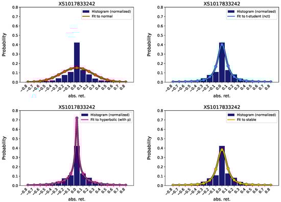
Figure 1.
Fitting of observed absolute returns of the price of a bond (ISIN XS1017833242)—represented in the histogram—to different probability density functions. Top, left: Normal; Top, right: Non-centered t-student; Bottom, left: Generalized hyperbolic; Bottom, right: Lévy stable.
Table 2.
Parameters of the fitting of the returns to normal probability distributions.
Table 3.
Parameters of the fitting of the returns to non-centered t-student (nct) probability distributions. Bold font indicates the best fitting among all four analyzed distributions.
Table 4.
Parameters of the fitting of the returns to generalized hyperbolic (g. hyp.) probability distributions. Bold font indicates the best fitting among all four analyzed distributions.
Table 5.
Parameters of the fitting of the returns to Levy stable probability distributions.
We will use the fitted distributions to generate synthetic data, which will be used for inferring properties of the ES of the returns of financial products. The usage of synthetic data has been encouraged by prestigious authors (López de Prado, 2018). In order to avoid too extreme values, we establish truncation values for the synthetic data. If the generated random numbers—which correspond to absolute returns of bonds—are above +30 or below −30 (note that the prices of bonds are usually measured so that they are about 100 currency units), then the generated synthetic datum is discarded, and another random number is generated. We deem these round values reasonable for bonds; for example, the bond with ISIN US33616CAB63 (First Republic Bank) fell over 23 in a single day in spring 2023. For the stocks of Shell, we set maximum and minimum truncation limits of log(1.4) and log(0.6), which are consistent with historical extreme values of oil companies (+36% of BP on 1969 June 4 and −47% of Marathon Oil Corporation on 2020 March 3). For the stock of Apple Inc we establish limits of log(0.48) and log(1.33), consistent with its historical extrema. These truncation limits () will also be used when we perform numerical integration to calculate the Expected Shortfall of probability density functions (this is using Equation (3) below with integration limit instead of ).
4.2. How the Expected Shortfall from Historical Simulation Depends on the Size of the Dataset
The Expected Shortfall is a risk measure equal to the conditional expectation of a return r (financial loss) given that r is below a specified quantile (Brazauskas et al., 2008). If the return r is considered to be a continuous random variable, then the Expected Shortfall can be defined as follows:
where is the probability density function of the return; is the value of the return such that , being the confidence level the number which represents the total probability of the most adverse returns to be considered in the calculation of the ES. The multiplicative factor is sometimes omitted from the definition of the ES; see, for instance, equation (8.52) of (McNeil et al., 2005). Other equivalent definitions exist, e.g., where indicates expected value, and ES, VaR is the Expected Shortfall and Value-at-Risk for confidence level of the analyzed return. To sum up, the Expected Shortfall provides the average expected loss for the worst-case scenarios (Acerbi & Tasche, 2002), with those scenarios depending on a predetermined threshold (for example, the 5% worst possible losses).
Despite definition (3), the Expected Shortfall is frequently calculated by considering just observed values of a given return . For example, the European Banking Authority (European Banking Authority, 2020) specifies the formula that follows for its calculation:
(this formula was found in Peracchi and Tanase (2008)) where the signs indicate the integer part (floor) of x and the indices (i) of are ordered so that are monotonically increasing; we set (2.5%). This way of proceeding ignores altogether other non-observed values of the returns. Such values were possible but did not take part in the calculation; hence, potentially important information is discarded. On the one hand, Equation (4) has the advantage that it does not require any assumption on the actual distribution of the returns (i.e., if it is normal, generalized hyperbolic, etc.). On the other hand, the cost of making this assumption may be to distort the calculated Expected Shortfall strongly. The arbitrariness of the choice of the underlying probability distribution can be partly mitigated by analyzing different ones, as we do in this research work.
To quantify whether the usage of Historical Simulation (Equation (4)) severely distorts the calculation of the ES, we proceed as follows. We fit the collection of returns of a given financial product for a given time range (see Table 1) to four different probability density functions. Among them, we choose the one whose loss function (Equation (2)) is minimal, i.e., which has the maximum likelihood (see numbers in bold in Table 3 and Table 4). We then generate synthetic datasets using the parameters of the chosen distribution. Each synthetic dataset consists of points. For each value of , we generate half a million synthetic datasets; for each of them, we calculate the ES using Equation (4). We then calculate the mean, median, standard deviation, and 95% confidence interval of this collection of 500 k ESs for each . For the returns of the analyzed BASF bond, these quantities are presented in Figure 2-top. The solid lines of the upper subplots clearly indicate that the average Expected Shortfall tends to increase in a monotonical manner with the sample size. It converges to steady values (plateau) for high values of but requires relatively high numbers of returns to approach it. For example, the mean and median of the ES of the synthetic data are far from their converged values for .
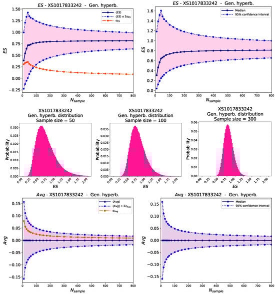
Figure 2.
Top: Relationship between the ES calculated using the historical method (HS) and the number of data points of the sample size. Left: Standard deviation (red) and average plus/minus twice the standard deviation (blue); Right: Median and 95% confidence interval. Center: Histograms of the expected shortfalls obtained with synthetic data of the absolute returns of a bond (ISIN XS1017833242) as a function of the number s of the generated random values for each ES calculation. Left: ; Center: ; Right: . Bottom: Relationship between the average of the synthetic data (identical to those of the top figures) and the number of data points of the sample size. Left: Standard deviation (red) and average plus/minus twice the standard deviation (blue); Right: Median and 95% confidence interval. The synthetic data was generated using a generalized hyperbolic distribution.
Such a monotonical increase is a consequence of the highly nonlinear definition of the Expected Shortfall. For example, if we calculate the average of the synthetic data instead of the ES, we will notice that there is no trend with the size of the dataset. This can be viewed in Figure 2-bottom, which presents the mean, median, standard deviation, and confidence interval of the average of each synthetic dataset that was used in the calculations for Figure 2-top. Here, the solid lines are horizontal; the sizes of the differences of the mean of the averages for different values of are far lower than the standard deviation (orange curve in Figure 2-top, left).
In the Supplementary Information, we present graphs similar to Figure 2, which correspond to the other financial products listed in Table 1. They all confirm that the average ES monotonically increases with the sample size until it reaches a plateau.
4.3. Expected Shortfall from Fitting to Small Datasets
The results presented in the previous section indicate that the usage of Historical Simulation (i.e., using observed values only) in the calculation of the ES is potentially inaccurate and prone to systematic errors (underestimation of the ES). This drawback can be mitigated by increasing the sample size. However, such a solution may not always be either feasible or accurate. Simply increasing the number of returns used in the HS calculation would probably require using older data, which may be stale. The economic conditions, as well as the inner operation of a company, tend to change over time; hence, the obsolescence of data may lead to inaccurate results. Moreover, there exist illiquid products, like many corporate bonds, for which the returns are unknown for many dates. In those cases, one is forced to perform calculations with few returns (datasets of small size), thus leading to potentially severe inaccuracies, as indicated by Figure 2 (which corresponds to absolute returns of a bond price) and by figures presented in the Supplementary Information. Can this inconvenience be overcome? In this section, we present a method to mitigate the problem.
Since the inaccuracies in the Expected Shortfall calculation are a consequence of not considering non-observed, though possible, extreme values, the impact of their neglect can be eased by finding an approximation to them. We can infer the probability density function from the analyzed dataset, as indicated above. Even if this dataset consists of a few points, the fitting will provide probabilities for extreme values, which can be used in the calculation of the Expected Shortfall.
We exemplify this way to proceed with the results displayed in Figure 3. In the plots on top, which correspond to the BASF bond, the dash-dotted lines correspond to the mean and median of the 2000 values of the ES of different sets of synthetic data using HS (from Equation (4)). The dashed lines represent the mean and median of the ES obtained by fitting each dataset to a generalized hyperbolic probability density function and then using such continuous functions to calculate the ES. Since the continuous probability density functions are less prone to underestimate the extreme values (tails) than Historical Simulation, the values of the dashed line are always above the values of the dash-dotted line. These results indicate that if we take the ES of the fitting to the large (whole) observed dataset (gray horizontal line in Figure 3-top) as our baseline, then fitting to probability distributions provides more accurate results than HS. The effect is especially strong for low values of the sample size.
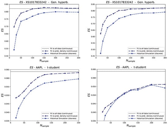
Figure 3.
Comparison of the mean (left) and median (right) of the Expected Shortfall of datasets of different sizes (). The dash-dotted curves (Historical Simulation) correspond to the ES of collections of observed returns calculated with Equation (4); the dashed curves correspond to ES calculated from fitting those collections of observed returns to fat-tailed distributions. Gray horizontal lines correspond to the ES from the fitted distribution of the whole dataset. The plots on top correspond to a BASF bond (fitted to generalized hyperbolic distributions); the plots on the bottom correspond to the AAPL stock (fitted to non-centered t-student distributions).
The analyzed bonds (BASF and Charles Schwab, which are liquid) can be considered proxies of other corporate bonds, which can be illiquid. We prefer to use such liquid bonds (proxies) in our analysis to account for illiquid bonds to avoid distortions in the price due to low supply and demand. Such distortions, often noticeable as large values of the bid-ask spreads of illiquid bonds, would increase the complexity of the products and thus opaque the ES-vs-sample size analysis, whose clear presentation is among the main goals of this paper. For illiquid bonds, just a few returns are known, and hence, taking values of a proxy (e.g., BASF’s) bond is expected to reasonably give an account of the modeled product (illiquid bond). However, this is not the case for stocks (shares of companies traded in stock exchanges). Though there exist many small companies whose stocks have very low trading volume (and may not be purchased even once a day), the vast majority of the volume of traded stocks corresponds to very liquid products, which are traded numerous times a day. Therefore, the fitting of observed data for calculating accurate ES may, in principle, not look necessary for stocks because their daily prices are known. Conversely, we think that the fitting procedure is also worthwhile for stocks. This is because the number of days to be used for calculating the ES ( in Equation (4)) is arbitrary. If one wants to calculate risks with a given horizon (e.g., 126 days, the usual number of trading days in a semester), the market conditions may have changed during that time, making the oldest data stale. In that case, it may be more appropriate to choose, e.g., 63 days instead. However, from our previous analysis (Figure 2-top), we know that such a small number of data would distort ES if calculated through historical simulation, leading to a non-converged value (below the plateau). Therefore, a wiser way to proceed would be to use recent data, to fit them to a fat-tailed distribution, and finally to calculate the ES of that distribution.
In Figure 3-bottom, we present data analogous to those of Figure 3-top, yet with the corresponding calculations performed differently. For every sample, with size (x-axis of the figures), we no longer randomly generated returns of the price of the analyzed product. In contrast, we took the last returns of the stock price. This was carried out for every single trading date of the analyzed time interval (see Table 1). Therefore, each point displayed in Figure 3-bottom is not the average of 2000 trials, but the average of a number of trials equal to the total number of returns of the time interval (5 years) minus .
In Figure 3-bottom, we also present a horizontal gray line that indicates the ES from the distribution fitted to the whole dataset. Note that this is just a reference; it does not need to be equal to the calculated values (blue lines). This is because the ES may abruptly change for sudden strong price drops. For example, if , the ES may be 0.05 the first year, 0.01 the second year, 0.03 the third year, etc., and the average of these numbers would not need to be the ES of the whole (5-year) dataset, which may closer to 0.05 if the strongest price dips concentrated in that period.
Fitting a dataset to probability density functions is more computationally demanding than a simple calculation of the ES using Historical Simulation. However, due to the capabilities of present-day computing facilities (García-Risueño & Ibáñez, 2012), such calculations are affordable. The calculations whose results are presented in this article were performed on a personal laptop (MacBook Pro 13-inch M1 2020, i.e., not on a cluster or other supercomputing facility) and were carried out within a few weeks. The code was run in Python 3.11, using recent versions of numpy and scipy.stats modules (Harris et al., 2020; Virtanen et al., 2020).
5. Conclusions
In this article, we have shown a presentation about how the method of Historical Simulation tends to systematically underestimate the Expected Shortfall of random variables like the returns of financial products. This phenomenon is due to the fact that observed sample datasets are forcedly finite and, hence, cannot cover the virtually infinite possible values that correspond to continuous probability distributions. This limitation has a low impact when calculating some quantities, like the sample average. However, it has a dramatic impact on the calculation of the ES, which strongly depends on the minimum values of the sample, which in turn tend to be lower for higher numbers of points in the sample. Our results indicate that potentially severe errors made using Historical Simulation may be frequent if the number of considered datapoints is not close to the number of trading days of a year; nevertheless, taking so much data may lead to staleness of the data (due to changes in the economic situation). This strongly advises against the usage of Historical Simulation for calculating the Expected Shortfall; we encourage Regulators to seriously consider the potential impact of such practice. We have indicated two methods to mitigate the inaccuracies in the ES: increasing the sample size and—most recommended—fitting the sample dataset to a continuous, fat-tailed probability density function (preferably the generalized hyperbolic density function) to be used for calculating the Expected Shortfall. This can be made using the code used for the calculations of this article, which is freely distributed. We expect that our research work provides insights on important statistical properties to Finance practitioners, and that it helps in their risk management activities.
Possible future research lines include considering other fat-tailed distributions, like Johnson’s , as well as more sophisticated fittings of the observed returns, e.g., based on autoregressive schemes or neural networks. A more comprehensive comparison of the parametric methods proposed in this paper with other parametric and non-parametric approaches using real market data for different kinds of financial products is also in scope.
Supplementary Materials
Supplementary Information containing additional equations and results can be downloaded at: https://www.mdpi.com/article/10.3390/jrfm18010034/s1.
Funding
This research received no external funding. The author carried out all the activities related to this paper independently of his job in banking and insurance, using his own time and resources. The views expressed in this article are solely those of the author and do not reflect the official position or views of VidaCaixa, CaixaBank or the University of Zaragoza.
Informed Consent Statement
Not applicable.
Data Availability Statement
The code employed in our calculations is publicly available in the github repository of the first author: https://github.com/pablogr/FIN_paper_ES_fat_tails, accessed on 6 January 2025. This code can be used to perform an analysis of the convergence of the ES for dates and financial products freely chosen by the user. It is freely distributed with the sole condition of citing its source and this article.
Acknowledgments
The author is grateful to Eduardo Ortas and to Jesús Asín (University of Zaragoza) for interesting discussion and revision of the manuscript, as well as to the anonymous reviewers of the submitted version, whose remarks nicely contributed to improve it.
Conflicts of Interest
The author declares no conflicts of interest. He also declares that he had jobs in banking and insurance during the time he carried out this research.
Abbreviations
The following abbreviations are used in this manuscript:
| CVaR | Conditional Value-at-Risk |
| ES | Expected Shortfall |
| HS | Historical Simulation |
| nct | non-centered t-student |
| probability density function | |
| VaR | Value-at-Risk |
References
- Acerbi, C., & Tasche, D. (2002). Expected shortfall: A natural coherent alternative to value at risk. Economic Notes, 31(2), 379–388. [Google Scholar] [CrossRef]
- Barzilai, J., & Borwein, J. M. (1988). Two-point step size gradient methods. IMA Journal of Numerical Analysis, 8(1), 141–148. [Google Scholar] [CrossRef]
- Brazauskas, V., Jones, B. L., Puri, M. L., & Zitikis, R. (2008). Estimating conditional tail expectation with actuarial applications in view. Journal of Statistical Planning and Inference, 138(11), 3590–3604. [Google Scholar] [CrossRef]
- Carrillo Menéndez, S., & Hassani, B. K. (2021). Expected Shortfall reliability-added value of traditional statistics and advanced artificial intelligence for market risk measurement purposes. Mathematics, 9(17), 2142. [Google Scholar] [CrossRef]
- Chen, X. F., & Chen, G. B. (2012). Pattern search for generalized hyperbolic distribution and financial risk measure. Applied Mechanics and Materials, 155, 424–429. [Google Scholar] [CrossRef]
- Chen, Y., Härdle, W., & Jeong, S.-O. (2008). Nonparametric risk management with generalized hyperbolic distributions. Journal of the American Statistical Association, 103(483), 910–923. [Google Scholar] [CrossRef][Green Version]
- Choudhry, M. (2013). An introduction to value-at-risk. John Wiley & Sons. [Google Scholar]
- European Banking Authority. (2020). Final Draft RTS on the calculation of the stress scenario risk measure under article 325bk(3) of regulation (EU) No 575/2013 (Capital Requirements Regulation 2—CRR2). EBA Publications. [Google Scholar]
- García-Risueño, P., & Ibáñez, P. E. (2012). A review of high performance computing foundations for scientists. International Journal of Modern Physics C (IJMPC), 23, 1230001. [Google Scholar] [CrossRef]
- García-Risueño, P., Ortas, E., & Moneva, J. M. (2023). The effect of fat tails on rules for optimal pairs trading. Available online: https://papers.ssrn.com/sol3/papers.cfm?abstract_id=4518354 (accessed on 9 January 2025).
- Hafez, P., & Lautizi, F. (2019). Machine learning and event detection for trading energy futures. In T. Guida (Ed.), Big data and machine learning in quantitative investment (pp. 169–185). John Wiley & Sons. [Google Scholar]
- Harris, C. R., Millman, K. J., van der Walt, S. J., Gommers, R., Virtanen, P., Cournapeau, D., Wieser, E., Taylor, J., Berg, S., Smith, N. J., Kern, R., Picus, M., Hoyer, S., van Kerkwijk, M. H., Brett, M., Haldane, A., del Río, J. F., Wiebe, M., Peterson, P., … Oliphant, T. E. (2020). Array programming with NumPy. Nature, 585(7825), 357–362. [Google Scholar] [CrossRef] [PubMed]
- Hellmich, M., & Kassberger, S. (2011). Efficient and robust portfolio optimization in the multivariate generalized hyperbolic framework. Quantitative Finance, 11(10), 1503–1516. [Google Scholar] [CrossRef]
- Johnson, N. L., Kotz, S., & Balakrishnan, N. (1995). Continuous univariate distributions, volume 2 (Vol. 289). John Wiley & Sons. [Google Scholar]
- Liu, M., & Staum, J. (2010). Stochastic kriging for efficient nested simulation of Expected Shortfall. Journal of Risk, 12(3), 3. [Google Scholar] [CrossRef]
- López de Prado, M. (2018). Advances in financial machine learning. John Wiley & Sons. [Google Scholar]
- Maio, S., Macri, P., & Maurette, M. (2017). Risk measurement using extreme values theory. Available online: https://papers.ssrn.com/sol3/papers.cfm?abstract_id=3829785 (accessed on 9 January 2025).
- McNeil, A. J., Frey, R., & Embrechts, P. (2005). Quantitative risk management: Concepts, techniques and tools. Princeton University Press. [Google Scholar]
- Nadarajah, S., Zhang, B., & Chan, S. (2014). Estimation methods for expected shortfall. Quantitative Finance, 14(2), 271–291. [Google Scholar] [CrossRef]
- Peracchi, F., & Tanase, A. V. (2008). On estimating the conditional expected shortfall. Applied Stochastic Models in Business and Industry, 24(5), 471–493. [Google Scholar] [CrossRef]
- Virtanen, P., Gommers, R., Oliphant, T. E., Haberland, M., Reddy, T., Cournapeau, D., Burovski, E., Peterson, P., Weckesser, W., Bright, J., van der Walt, S. J., Brett, M., Wilson, J., Millman, K. J., Mayorov, N., Nelson, A. R. J., Jones, E., Kern, R., Larson, E., … SciPy 1.0 Contributors. (2020). SciPy 1.0: Fundamental Algorithms for scientific computing in Python. Nature Methods, 17, 261–272. [Google Scholar] [CrossRef] [PubMed]
- Wong, W. K. (2008). Backtesting trading risk of commercial banks using Expected Shortfall. Journal of Banking & Finance, 32(7), 1404–1415. [Google Scholar]
Disclaimer/Publisher’s Note: The statements, opinions and data contained in all publications are solely those of the individual author(s) and contributor(s) and not of MDPI and/or the editor(s). MDPI and/or the editor(s) disclaim responsibility for any injury to people or property resulting from any ideas, methods, instructions or products referred to in the content. |
© 2025 by the author. Licensee MDPI, Basel, Switzerland. This article is an open access article distributed under the terms and conditions of the Creative Commons Attribution (CC BY) license (https://creativecommons.org/licenses/by/4.0/).