Long-Run Trade Relationship between the U.S. and Canada: The Case of the Canadian Dollar with the U.S. Dollar

Abstract

This study investigates the long-run relationship between the U.S. dollar and the Canadian dollar by analyzing the bilateral exchange rate induced by nominal and real shocks. The methodology centers on a structural vector autoregressive (SVAR) model, including the analysis of impulse response and variance decomposition to account for the impact of nominal and real shocks on exchange rate movements. This study also decomposes real shocks into demand and supply factors from both Canada and the U.S. and compares their impacts on the nominal and real exchange rates. The results are compared to shocks driven by country-specific nominal factors. This study uses quarterly data from December 1972 to December 2023. The findings suggest that real shocks have a permanent impact on both the nominal and real exchange rates, compared to nominal shocks, which have a temporary impact. Country-specific real supply-side factors have a more significant impact than country-specific real demand-side factors. Country-specific nominal factors barely impacted the nominal and real exchange rates between the U.S. and Canada.

1. Background to Study

Five keywords are making the buzz in the headlines nowadays. Dubbed the 5Ds, they are deglobalization, decarbonization, demographics, debt, and dovish policies (Moulle-Berteaux 2023). These secular factors are directly contributing to inflation, at a structural level, in major developed economies, including Canada and the U.S. Since COVID-19, deglobalization and decarbonization have added to the volatility of prices globally. For instance, while the consumer price index (CPI) changed from 1.2% in 2020 to 8% in 2022 before decreasing by 4.1% year-over-year, Canada also experienced a similar trend, with the CPI changing from 1.4% in 2020 to 6.8% in 2022, before falling by 3.9% in 2023. During the same period, the trade balance relative to the Gross Domestic Product (GDP) ranged between −3.9% (2023) and −4.6% (2022) in the U.S. Comparatively, Canada has, after 10 years of experiencing negative values, started to continuously report positive trade balances, ranging between 0.4% and 1.2% of the nation’s GDP. Post-COVID-19, both developed economies reported real GDP, which increased, on a year-to-year basis, at a decreasing rate, with the U.S. (Canada) real GDP increasing at 2.5% (1.1%), respectively (Factset 2024). Further, while the wholesale price indices (WPI) for both countries showed a positive correlation, the nominal exchange rate between the Canadian dollar fluctuated between 0.7 U.S. dollars (USD) per Canadian dollar (CAD) to 0.8 USD during the period of 2020-early 2024. Finally, imports have been dropping for both developed entities, with the U.S. (Canada) experiencing a fall of 4.9% (2.2%) in 2023. In the same vein, exports dropped in the U.S. (Canada) by 2.2% (5%). Energy commodities such as crude oil have not been spared either, with the West Texas Intermediate (WTI) crude oil futures price fluctuating from USD 20 per barrel in 2020 to a settlement price of USD 103.89 in March 2022 and trading around USD 80 per barrel in early 2024 (Chicago Mercantile Exchange Group 2024).

One of the major causes of price volatilities in commodities can be attributed to government actions regarding climate change and investors gradually orienting their investments toward sustainable equity finance (Gurrib et al. 2023). While government-based initiatives on speedier decarbonization and reduced greenhouse emissions are plentiful, with notable international cooperation among various key global players such as the U.S. and Canada (Plotnick 1963), the mechanisms driving the green transition have also shifted focus to local initiatives. For instance, the rise in the implementation of carbon pricing and increased interest in local renewable energies led to various countries adopting protectionist measures as a fuel for deglobalization. While globalization brought a delocalization of production to geographical areas with lower costs of production and lower environmental standards, policymakers in the U.S. are promoting the adoption of strategies to bring production back to the leading nation. As an example, the Inflation Reduction Act necessitates that part of a product is U.S.-made. Sánchez (2023) posits that while on-shoring or near-shoring the production of strategic goods such as minerals can allow countries to benefit from lower transportation costs and avoid supply chain issues, multilateralism is recommended by sanctioning countries that pursue aggressive trade policies or wars against other countries.

Alternatively stated, post-COVID-19 supply chain disruptions, the Russia–Ukraine war and the U.S.–China trade war can be attributed as major causes of fluctuations in current trade activities and commodity prices globally. Increases in energy commodity prices, particularly in crude oil and natural gas, affect each nation differently based on whether the economy is an importer or exporter of commodities in general (Lee and Hussain 2023). For instance, exchange rate fluctuations for commodity currencies, such as the Australian dollar, were primarily driven by gas price shocks resulting from the ongoing war in Ukraine (Sokhanvar and Lee 2023).

Canada is of particular interest, as it is a major consumer, producer, and exporter of energy. Specifically, Canada is among the top ten producers of natural gas, oil, hydropower, uranium, nuclear power, biofuels, and wind. Energy contributes to 10% of the country’s GDP, with the petroleum and electricity industries contributing 7.2% and 1.7% (Natural Resources Canada 2023). The energy sector also represents a major stream of capital investments and trade flows. Even though the country has a broad range of free trade agreements with about 70% of the global economy, demand for exports has been mostly driven by the U.S. While it can be argued that the termination of the North American Free Trade Agreement (NAFTA) had a negative impact on Canadian exports, the effect was offset by the Canada–United States–Mexico Agreement (CUSMA) in mid-2020 (Global Affairs Canada 2020). With major industries based in the primary sector, Canada is the fourth (fifth) largest producer of crude oil (natural gas) globally, with the third largest oil reserves. More than 95% of its oil is exported to the U.S. (Canadian Association of Petroleum Producers n.d.). Conversely, 60% of U.S. imports come from Canada. In addition to its huge reserves of natural gas, Canada is the fourth largest metallurgical coal exporter, after Australia, Russia, and the U.S. (Government of Canada 2024). A total of 100% of Canada’s exported electricity is destined for the U.S., with 92% of the electricity imported by the U.S. from Canada. Finally, Canada is the second largest exporter of uranium globally (Canada Nuclear Safety Commission 2023), with 64% of its exports heading to the U.S. and Europe (Canada Action 2024).

In light of the critical importance of the energy sector in Canada, the trade dynamics between Canada and the U.S., and several additional factors that are currently affecting the global financial markets, including deglobalization; localized decarbonization with Canada’s sustained commitment to the phase-out of conventional coal-fired electricity nationally by 2030 (International Energy Agency 2022); the Russia–Ukraine war; and the U.S–China trade war, it is imperative to investigate the relationship between the Canadian dollar and U.S. dollar. Specifically, it is also valuable to understand which country-specific factors drive the exchange rate between the two countries, especially given that they are important trading partners to each other; both countries are leading consumers, producers, and exporters of energy globally; and the Canadian dollar per U.S. dollar is one of the most actively traded currency pairs.

While it is expected that a structural model constructed to determine exchange rates should be able to shed light on variables that contribute to nominal and exchange rate changes, evidence from the extant literature is mixed. For instance, Kim and Enders (1991) and Baillie and McMahon (1989) find no cointegrating relationships between bilateral exchange rates and various macroeconomic indicators. Comparatively, Dibooglu and Enders (1995) and Butt et al. (2023) found more significant relationships between macroeconomic factors such as oil price, interest rates differentials and exchange rates. Importantly, Meese and Rogoff (1983) and Frankel and Rose (1995) support that macroeconomic models can be limited in terms of the information included in exchange rate determination.

Instead of regressing macroeconomic variables onto exchange rates, we borrow and extend (Enders and Lee 1997) by adopting the technique proposed by (Blanchard and Quah 1988) to defragment exchange rate movement into the changes induced by nominal and real factors. A similar notable study is (Nakatani 2017), which examined the effects of real shocks and financial shocks on exchange rates in emerging markets, where productivity shocks were used as shocks in the real sector and risk premium shocks as financial shocks. The latter found that although both productivity shocks in the real sector and risk-premium-based shocks from financial markets affect exchange rates in emerging markets, the impact of shocks depends on crisis periods. Importantly, the author points to the significant effect of monetary policy can have on exchange rates.

For our study, we decompose the Canadian dollar relative to the U.S. dollar into movements caused by nominal shocks compared to those caused by real shocks. Our primary contribution is to further understand the long-run relationship between the Canadian dollar and the U.S. dollar in an unprecedented period backed by deglobalization and decarbonization. Specifically, we showcase the differential impacts of real and nominal shocks using impulse responses and variance decompositions on nominal and exchange rates. In line with the prior literature, we further decompose the real shocks into demand- and supply-driven factors and analyze the impact of these country-specific factors on the nominal and real exchange rates. This also enables us to compare country-specific real demand and supply shocks to country-specific nominal shocks in the exchange rate.

We differ from (Enders and Lee 1997) and (Nakatani 2017) in two important aspects. Firstly, we are extending the data analysis from 1973–1992 to December 1972–December 2023, thereby giving us a more important gauge of the long-run relationship between the two countries’ currencies. Secondly, we are analyzing the effect of real government expenditure, real GNP, and nominal money supply on the nominal and real exchange rate, compared to (Enders and Lee 1997), who analyze the impact of the ratio of log real government expenditure in one country relative to the other country, the ratio of log real GNP between both countries, and the ratio of log nominal money supply between the two countries, and (Nakatani 2017), who used productivity shocks to capture shocks in the real economy, and risk premium shocks as financial shocks. Specifically, we use real government expenditure as a measure of demand shock and real GNP as a supply shock, while retaining the money supply (M2) is used as a nominal shock. Since we are more interested in the impact of country-specific shocks on the real and nominal exchange rate, we retained the use of the log of demand/supply variables and money supply factors from Canada and the U.S. Last, but not least, Nakatani’s (2017) notable study focused on the exchange rates of emerging markets during crises compared to our focus on the Canadian/U.S. exchange rate.

The rest of the paper is organized as follows: Section 2 provides some literature reviews on exchange rate determination, commodity currencies, real and nominal exchange rates, and the demand and supply factors affecting exchange rates. Section 3 summarizes the methodologies and data used. Section 4 provides the data and some preliminary analysis. Section 5 provides the research findings. We rest our case with some concluding remarks.

2. Literature Review

2.1. Exchange Rate Determination

The U.S. and Canadian dollars are major world currencies and as such have drawn a significant amount of attention in academia. There exist swathes of research that examine the relationship between the two currencies using different methodologies. The effects of oil shocks on the U.S. exchange rate have been well-documented (Ji et al. 2020; Malik and Umar 2019). A new adjusted relative strength index was employed to study the connection between energy markets and exchange rates in the findings suggest an inverse relationship between energy and currency markets. Other commodities such as gold have also impacted the currency exchange rates (Jia et al. 2023).

Trade is a major factor in determining the exchange rate. Dogru et al. (2019) show the role the balance of trade plays in determining the exchange rates. Covered interest parity and contractions of cross-border bank lending in dollars were shown to go hand in hand with the strong U.S. dollar (Avdjiev et al. 2019). The authors reveal the role of the dollar as a key barometer of risk-taking capacity in global capital markets. Bussière et al. (2020) report that quantity elasticities are significantly below one and export prices are significantly affected by exchange rate changes. Bruno and Shin (2023) show the interaction between the U.S. dollar and international trade. The study reveals a novel channel of exchange rate transmission that goes in the opposite direction to the competitiveness channel.

Monetary and fiscal policy have been studied as major drivers of the exchange rate. The effects of monetary policy regime on the relative importance of nominal exchange rates were studied by (Eichenbaum et al. 2021) who found that the current real exchange rate predicts future changes in the nominal exchange rate. The effects of monetary policy announcements on exchange rate dynamics in the U.S. have been studied by (Gründler et al. 2023). The results suggest that while the short-run effects on the exchange rate are mainly due to policy shocks, the medium-run response is guided by information effects. Similarly, the effect of monetary policy surprises on the exchange rate behavior was studied by (Gürkaynak et al. 2021), who found that conditioning on possible information effects driving longer-term interest rates, there appears to be additional drivers of exchange rates. Fiscal shocks such as government spending have been shown to affect the real exchange rate. The study by (Bénétrix and Lane 2013) implies that the impact of public sector expenditure changes across different types of spending, with shocks to public investment generating larger and more persistent real appreciation than shocks to government consumption.

Global shocks have also been shown to affect the exchange rates. The effects of extreme events such as COVID-19 and the war in Ukraine have been studied (Hanif et al. 2023; Sokhanvar et al. 2023). Greenwood et al. (2023) developed a model in which specialized bond investors must absorb shocks to the supply and demand for long-term bonds in two currencies. Their proposed model matches several important empirical patterns. Empirical patterns include the co-movement between exchange rates and term premia. The study also finds that central banks’ quantitative easing policies affect exchange rates.

2.2. Real and Nominal Shocks

Fisher and Huh (2002) document the sensitivity of exchange rate and trade balance to real shocks such as supply and demand disruptions. In the case of highly interconnected economies like Canada and the USA, the demand shocks may lead to a substantial fluctuation in the bilateral exchange rate due to changes in import and export levels. This also applies to supply shocks like the change in natural resources availability, geopolitical stability, natural disasters, or technological advancement that directly affect the production capacity and trade flow between countries, such issues can significantly and immediately affect the bilateral exchange rate (Sarangi et al. 2022). For instance, the fluctuation in oil prices may cause an immediate and significant demand shock. In detail, the increase in oil prices will lead to an appreciation of the CAD relative to the USD since the Canadian economy relies on oil exports (Youssef and Mokni 2020). On the supply side, unexpected and sudden changes in the production level due to technological advancement or disruptions in supply chains (e.g., COVID-19) or natural disasters can cause a supply shock. These shocks have a variant impact on the currency exchange rates through the change in the prices of goods and services between the two countries.

On the other hand, the monetary approach to exchange rate theory is the main source of information about the link between money supply and exchange rates. According to this theory, a currency’s supply and demand, which are impacted by variables like interest rates, inflation forecasts, and economic growth, determine its price (Adaramola and Dada 2020). This theory states that, all else being equal, a rise in a nation’s money supply raises inflation and decreases demand for that nation’s currency, which causes it to weaken. Thus, when the money supply is reduced, foreign capital tends to be attracted to higher interest rates and lower inflation rates, which leads to currency appreciation (Mussa 1976; Frenkel 1976). This perspective is also empirically supported, studies utilizing structural Vector Auto-Regression (VAR) models and cointegration analysis indicate that demand and supply shocks can cause significant and long-term changes in the behavior and dynamics of currency exchange rates (Zhou 1995).

Exchange rate fluctuations also might be affected due to nominal shocks, which typically arise from the change in money supply and the country’s monetary policy. For instance, inflation expectations and interest rates are directly and positively associated with the money supply, causing an increase in inflation and depreciating the currency value. This depreciation can initially have a negative impact on countries’ trade balance, as imports become more expensive, and exports increase without experiencing a corresponding growth in foreign demand. However, the long-term effects of these nominal shocks can vary depending on the elasticities of demand for traded goods and the speed at which prices adjust in both local and foreign markets. These effects are vital to exploring and understanding the nominal dynamics between the CAD and USD. In the context of CAD and USD, (Sarno and Taylor 2001) delve deeply into this dynamic, explaining how policy differences between the Federal Reserve and the Bank of Canada can cause notable fluctuations in exchange rates. Research has indicated that significant swings in the CAD/USD exchange rate might result from divergences in the monetary policy outlook between the Federal Reserve and the Bank of Canada. For instance, the U.S. dollar is likely to depreciate relative to the Canadian dollar if the Canadian monetary policy is contractionary and the U.S. monetary policy is expansionary (Lane and Milesi-Ferretti 2007).

The other literature has discussed the impact of real government expenditure and currency demand shocks and documented that these two factors are pivotal in determining the exchange rate dynamics between the CAD and USD (Lavoie and Seccareccia 2006). In this regard, real domestic currency depreciation is typically the result of expansionary fiscal policy, which is shown in more government expenditure. This is because such spending usually results in more aggregate demand than supply, which drives up local prices in comparison to overseas prices and lowers the real exchange rate. Particularly, the government spending, monetary policy, and the real exchange rate align with the above discussion, as an increase in government purchases leads to a decline in the currency exchange rate due to the change in the country’s balance of payments and the goods and market equilibrium conditions (Bouakez and Eyquem 2015).

2.3. Structural Vector Autoregressions

Recently, machine learning has been actively applied to model financial asset movements (Gurrib and Kamalov 2022; Kamalov et al. 2021). Particularly, it has been widely used to model exchange rate time series. Kamalov and Gurrib (2022) compared the performance of ten machine learning algorithms to forecast instances of significant fluctuations in currency exchange rates. The study finds that the proposed outlier detection methods substantially outperform traditional machine learning and finance techniques. Similarly, Mao et al. (2024) compared several machine learning models to explore the predictability of exchange rate trends and found that a combination of a long short-term model and convolutional neural network outperformed the Transformer model.

Structural vector autoregressions (SVARs) are a key type of time series model widely utilized for macroeconomic analysis. It is a well-established approach with solid theoretical underpinnings and a wide range of applications (Arias et al. 2018; Carriero et al. 2019). This model includes multiple linear autoregressive equations that capture the combined movements of economic variables. The residuals from these equations are blends of fundamental structural economic shocks, which are presumed to be orthogonal (Kilian 2013). With a limited number of assumptions, it is possible to estimate these relationships—known as shock identification—and describe the variables through linear equations of both current and past structural shocks. The coefficients in these equations, termed impulse response functions, depict how the variables in the model react dynamically to shocks. Various methods for identifying structural shocks have been discussed in the academic community, including short-run restrictions, long-run restrictions, and sign restrictions (Charfeddine and Barkat 2020; Liu et al. 2020; Yıldız et al. 2021).

However, despite SVAR’s advantages, the model still has certain limitations. First, there is the reliance on identification restrictions, which often require strong assumptions, such as the long-run neutrality of certain shocks, to distinguish between structural shocks. These assumptions may not always hold, potentially leading to biased or incorrect interpretations of the results (Baumeister and Hamilton 2019). Additionally, SVAR models can be sensitive to the choice of variables and lag length, and incorrect specifications may result in misleading conclusions.

SVAR models are frequently used to explore how macroeconomic shocks affect economies and to evaluate economic theories. Baumeister and Hamilton (2019) use SVAR with a less restrictive formulation to analyze the impact of shocks on oil supply and demand. The author finds that supply disruptions are a bigger factor in historical oil price movements and inventory accumulation a smaller factor than implied by earlier estimates. SVAR models have been particularly focused on examining the impacts of monetary and fiscal policy shocks, along with other nonpolicy shocks such as those related to technology and finance. Suhendra and Anwar (2022) employed SVAR to study the response of asset prices to monetary policy shock in Indonesia. These results suggest that an increase in monetary policy interest rate appreciates the exchange rate, lowers the stock price, and reduces bond yields. The SVAR model was used to investigate structural shocks in monetary policy, exchange rates, and stock prices in Iran. The results suggest that a structural shock on the exchange rate does not affect the stock price, but the monetary policy’s structural shock positively impacts the real exchange rate. Recently, the effects of COVID-19 on the price of SP500 were investigated by using an SVAR model. The results imply that a 1% increase in cumulative daily COVID-19 cases in the U.S. leads to an approximately 0.01% cumulative reduction in the S&P 500 Index after 1 day (Yilmazkuday 2023).

3. Methodology

3.1. Nominal and Real Shocks

As mentioned earlier, this study borrows and extends the study from (Enders and Lee 1997), which is based on the theoretical concepts laid out in (Blanchard and Quah 1988). Specifically, the theoretical framework from (Blanchard and Quah 1988) assumes that the first disturbance (shock) has no long-run effect on output and employment, while the second disturbance (shock) has no long-run effect on unemployment but may have a real effect on output. Given further that these shocks are uncorrelated over different leads/lags, these assumptions define these shocks. The authors demonstrate that the shocks with permanent effects are supply-related shocks and those with temporary effects are demand-related shocks using a traditional Keynesian view of fluctuations. Further, the orthogonality assumption that the demand and supply shocks are uncorrelated does not restrict the channels through which demand, and supply shocks affect output and unemployment. A similar study assumes that neither supply nor demand shocks have a permanent impact on unemployment, but both shocks can have a permanent effect on the output level (Evans 1987).

Under an exchange rate determination framework, the methodology from Blanchard-Quah’s study is first adopted by (Enders and Lee 1997) since it enables a decomposition of changes in nominal and real exchange rates into the movements caused by nominal and real shocks. The exact type of nominal shock is left unspecified, with however the characteristic of having no long-lasting effect on the exchange rate. In line with (Blanchard and Quah 1988), although if the real rate is treated as non-stationary, the restriction that the total of the coefficients on lagged and current values of nominal disturbances in the real exchange rate model requires that nominal shocks have only transitionary effect on real exchange rates. This is analogous to the concept of money neutrality in the long run. Residual changes in the real exchange rates are attributed to real shocks. Moreover, the factorization used in (Enders and Lee 1997) requires the use of 2 series (bivariate vector autoregressive equations) to identify the 2 types of shocks. The variance and covariance of the residuals from both equations are used to identify the two shocks. While a practical view of the global economy would be exposed to many different types of disturbances, thereby limiting the identification of at most two types of shocks in a 2 × 2 system, (Enders and Lee 1997) summarize that the 2 × 2 model, given some identification restrictions are imposed, is aligned with a wide range of open economy structural macroeconomic models. The Dornbusch overshooting model (Dornbusch 1976) helps to illustrate the different kinds of shocks and the identification restriction related to the non-lasting impact of nominal shocks on real variables. The model supports those real shocks (whether they originate from changes in aggregate supply or demand) can impact both nominal and real exchange rates. Permanent changes in supply or demand will result in permanent changes in nominal and real exchange rates. Comparatively, nominal shocks, such as changes in money supply within the local economy, can affect real variables only temporarily but can impact other nominal variables in the long run. Alternatively stated, a permanent change in the money supply can permanently impact the nominal exchange rate but have only a short-term effect on the real exchange rate. This is consistent with many conventional open economy macroeconomic models in multinational finance. While we do not replicate the illustration of (Enders and Lee 1997) on the different impacts of nominal and real shocks on an economy, some important findings from the application of the Dornbusch model need to be stated. The money supply shock has a proportional effect on the nominal exchange rate but no effect on the real exchange rate. Government expenditure and income shocks however have a permanent on both the nominal and real exchange rates. Alternatively stated, there are shocks that affect both the nominal and real exchange rates in the short run. However, as time passes by, some shocks will have no effect on the real exchange in the long run but may have a permanent effect on the nominal exchange rate. The model and its variables are all consistent with the concept that nominal shocks can have a permanent (temporary) on the nominal (real) exchange rate. Like (Enders and Lee 1997), we use the log of U.S. Real GNP to CAD real GNP as a supply shock measure, the log of U.S. real government expenditure to CAD real government expenditures to capture demand shock, and the log of U.S. nominal money supply (M1) relative to CAD nominal money supply as a proxy for nominal shock.

3.2. Nominal and Real Exchange Rate

While a nominal exchange rate reflects the price of one currency against another, the real exchange rate (RER) attempts to measure the value of a country’s goods against those of another country, a group of countries, or the rest of the world at the prevailing nominal exchange rate (Carrière-Swallow et al. 2021; Kelesbayev et al. 2022; Ahmad et al. 2023). RER is expressed as follows:

$${RER}_{xy}={NER}_{xy}\times {\displaystyle \frac{{WPI}_x}{{WPI}_y}},$$

(1)

where ${RER}_{xy}$ is the real exchange rate between 2 countries (x and y), ${NER}_{xy}$ is the nominal exchange rate, and ${\displaystyle \frac{{WPI}_x}{{WPI}_y}}$ is the wholesale price ratio between the 2 countries. For example, the real exchange rate between the U.S. and Canada would be ${RER}_{USDCAD}={NER}_{USDCAD}\times {\displaystyle \frac{{WPI}_{US}}{{WPI}_{CAD}}}.$

The wholesale price index (WPI), as opposed to the consumer price index (CPI), focuses on the price of goods traded by corporations (Demir and Razmi 2022).

3.3. Structural VAR Model

In this study, we adopt a linear vector autoregression (VAR) model to explore the relationships among variables under consideration. The linear VAR model is employed based on its common acceptance and applied in the analysis of macroeconomic time series data (Enders 2014; Sims 1980). Linear VAR models grant apparent and interpretable results, which are crucial for understanding the underlying economic dynamics between the U.S. and Canadian dollars. Even though nonlinear relationships might exist, previous literature has shown that linear models are often sufficient to capture the key interactions in similar contexts (Kilian and Lütkepohl 2017). Therefore, we maintain the assumption of linearity, recognizing that it aligns with the objective of our study to analyze the long-run impacts of real and nominal shocks on exchange rates.

Assume ${\in }_{\mathit{r}\mathit{t}}$ and ${\in }_{\mathit{n}\mathit{t}}$ are the zero-mean mutually uncorrelated real and nominal shocks, respectively. Formally, a 2 × 1 vector of the first differences in real and nominal exchange rates, ${z_t=[∆r_{t,}∆e_t]}^{\prime }$, can be illustrated with a bivariate moving average representation as follows:

$$z_t\equiv {[∆r_{t,}∆e_t]}^{\prime }=B\left(L\right){\in }_t$$

(2)

$$\left[{\displaystyle \genfrac{}{}{0pt}{}{∆r_t}{∆e_t}}\right]=\left[\begin{array}{c}\begin{array}{cc}{B}_{11}\left(L\right),& B_{12}\left(L\right)\\ B_{21}\left(L\right),& B_{22}\left(L\right)\end{array}\end{array}\right] \left[\begin{array}{c}\begin{array}{c}{\in }_{rt}\\ {\in }_{nt}\end{array}\end{array}\right]$$

(3)

where $r_t$ is the real exchange rate at time period t; $e_t$ is the nominal exchange rate at time t; ${\in }_t={\left[\begin{array}{c}{\in }_{rt},{\in }_{nt}\end{array}\right]}^{\prime }$ $;{\in }_{rt}$ is the real shock at time t; ${\in }_{nt}$ is the nominal shock at time t; $B_{ij}\left(L\right)$ for i, j = 1, 2 is an infinite-order polynomial in the lag operator L; $∆$ is the first-difference operator; and the innovations are normalized such that Var(${\in }_t)$ = I. The time paths of the effects of the various shocks on the real and nominal exchange rates are implied by the coefficients of the polynomials $B_{ij}$(L). The restriction that the nominal shocks have no long-run effect on the real exchange rate is represented by the restriction that the sum of the coefficients in $B_{12}\left(L\right)$ sum to zero; thus if $b_{ij}\left(k\right)$ is the kth coefficient in $B_{ij}\left(L\right):$

$$B_{12}\left(L\right)\equiv {\sum }_{j=0}^{\mathrm{\infty }}{b}_{12}\left(j\right)L^j \mathrm{a}\mathrm{n}\mathrm{d} {\sum }_{j=0}^{\mathrm{\infty }}{b}_{12}\left(j\right)=B_{12}\left(1\right)=0$$

(4)

Since $b_{12}\left(j\right)$ is the effect of ${\in }_n$ on $∆r$ after j periods, ${\sum }_{j=0}^{\mathrm{\infty }}{b}_{12}\left(j\right)$ is the cumulative effect of ${\in }_n$ on $∆r$ over time. Similarly, because ${r_t=\left(1-L\right)}^{-1}{B}_{11}\left(L\right){\in }_{rt}+{\left(1-L\right)}^{-1}{B}_{12}\left(L\right){\in }_{nt}={\sum }_{k=0}^{\mathrm{\infty }}{\sum }_{j=0}^k{b}_{11}\left(j\right){\in }_{rt-j}+{\sum }_{k=0}^{\mathrm{\infty }}{\sum }_{j=0}^k{b}_{12}\left(j\right){\in }_{nt-j},{\sum }_{j=0}^{\mathrm{\infty }}{b}_{12}\left(j\right)$ is the effect of ${\in }_n$ on $r$ in the long run. Subsequently, the restriction that $B_{12}\left(1\right)\equiv {\sum }_{j=0}^{\mathrm{\infty }}{b}_{12}\left(j\right)=0$ implies that the cumulative effect of ${\in }_n$ on $∆r$ over time is zero, and that is the long-run effect of ${\in }_n$ on r is zero. Alternatively stated, the nominal shock ${\in }_n$ has only short-run effects on the real exchange rate, whereas the real shock ${\in }_r$ may have long-run effects.

4. Data

In addition to the important role Canada plays in the global arena and with its U.S. counterpart, it is important to understand the two countries’ relative importance in trade. Consistent with (Gurrib and Kamalov 2019), the Canadian dollar and the U.S. dollar are among the most actively traded currency pairs as per the Bank of International Settlements triennial 2022 survey (Bank for International Settlements 2022). Specifically, Figure 1 reports that, during the 2001–2022 period, the Canadian dollar represented between 4 and 5% of all foreign currency trades, with a noticeable increase to 6.2% in 2022. Comparatively, the U.S. dollar remains the dominant currency globally, being present in between 85% and 90% of all trades.

Figure 2 displays the RER for Canada relative to the U.S. Due to the wholesale price index in Canada being always higher than in the U.S., this resulted in a lower RER. While this relationship has been maintained during the whole period under study, the spread between the NER and RER displays less (more) volatility in the short-run (long-run). From Figure 2, we interpret there are two kinds of shocks which we dub as nominal and real shocks. While the real shock affects both NER and RER in a similar way, the nominal shock affects the two rates distinctively. Consistent with the concept of long-run neutrality (King and Watson 1992), we assume the nominal shocks to have a temporary effect on RER. Alternatively stated, permanent changes in nominal variables have no effect on real variables in the long run.

This serves as the identification restriction to defragment the exchange rates time series. To remove the effect of outliers in the data, we use the log of U.S. Real GNP to CAD real GNP as a supply shock measure (y), the log of U.S. real government expenditure to CAD real government expenditures to capture demand shock, and the log of U.S. nominal money supply (M1) relative to CAD nominal money supply as a proxy for nominal shock. All data were sourced from Factset.

Preliminary Analysis

Descriptive statistics including mean, median, standard deviation, skewness, kurtosis, the Jarque-Bera test for normality, the Augmented Dickey–Fuller (ADF) test, and the number of counts in each sample series are reported in

Table 1. Descriptive statistics.

	WPI_CA	WPI_U.S.	Nominal USD/CAD	Real USD/CAD	WPI-U.S./ WPI-CA
Mean	391.678	330.030	1.237	1.043	0.849
Median	401.115	310.709	1.244	1.052	0.856
Standard deviation	142.439	121.213	0.158	0.088	0.057
Kurtosis	−0.331	−0.602	−0.650	−0.783	−0.549
Skewness	−0.049	0.190	0.083	−0.075	0.250
Jarque-Bera	1.019	4.319	3.843	5.427	4.713
p-value	0.601	0.115	0.146	0.066	0.095
ADF	−0.358	0.244	−0.1250	−2.5970	−2.6080
p-value	0.9124	0.9747	0.2350	0.0953	0.0930
Observations	205	205	205	205	205
	U.S. Real Gov. Exp.	CA Real Gov. Exp.	U.S. Real GNP	CA Real GNP	U.S. Money Supply	CA Money Supply
Mean	2752	336	13.230	1.120	6483.614	706.313
Median	2709	313	12	0.905	4184.100	449.658
Standard deviation	669	84	5	0.750	5543.982	639.924
Kurtosis	−1.267	−0.864	−1.265	−0.766	0.765	0.639
Skewness	−0.199	0.353	0.186	0.546	1.258	1.229
Jarque-Bera	15.068	10.634	14.853	15.187	59.052	55.070
p-value	0.001	0.005	0.001	0.001	0.000	0.000
ADF	−0.4620	1.5730	1.4430	2.9980	2.7830	3.7530
p-value	0.8946	0.9995	0.9991	1.0000	1.0000	1.0000
Observations	205	205	205	205	205	205

Note: Table 1 summarizes the descriptive statistics for the U.S. and Canadian wholesale price indices (WPI_U.S. and WPI_CA), wholesale price ratio for USD/CAD, nominal exchange rate (NER) and real exchange (RER) for the Canadian dollar relative to the U.S. dollar (USD/CAD), real government expenditures for U.S. and Canada, and the real GNP and money supply for U.S. and Canada. Real government expenditures, real Gross National Product (GNP) and money supply are in billion. M2 is used as the measure of money supply. In total, 205 quarterly-based observations are collected from Factset for December 1972–December 2023.

for the period of 29 December 1972 to 29 December 2023. We use M2 as a measure of money supply in line with (Huang 2020) who finds the indicator, compared to other money supply indicators, to have a significant impact on economic growth in the short run. GNP, as opposed to Gross Domestic Product (GDP), as the size of the commodities sector and export orientation are two critical factors that could render GNP significantly different from GDP (Tan et al. 2022). The average WPI for Canada was higher than its U.S. counterpart, resulting in wholesale price ratios which pushed the real exchange rate (RER) between the U.S. and Canadian dollar to be lower than the nominal exchange rate (NER).

Although the average real government expenditure from the U.S. is almost 9 times that of Canada, normalizing each country’s average with its own standard deviation results in an average/standard deviation value of 4.11 and 3.97 for the U.S. and Canada, respectively. Apart from the money supply for both countries, all variables exhibited negative kurtosis, with U.S. real government expenditure and U.S. real expenditure having the lowest kurtosis values. WPI for Canada (U.S.) was negatively (positively) skewed. The nominal (real) exchange rate for USD/CAD was positively (negatively) skewed. Except for U.S. real government expenditure, all other government expenditures, real GNPs, and money supplies were positively skewed, with the latter exhibiting the highest skewness. The p-value under the Jarque-Bera test rejects the hypothesis of normality for all series, except for WPI for both countries and the nominal exchange rate for USD/CAD. Except for the RER and wholesale price indices ratios, the p-values under the Augmented Dickey–Fuller (ADF) test at a 10% significance level support that all the series are non-stationary at a 5% significance level. This is in line with Dornbusch (1976), where long-run restrictions in a structural vector require at least one non-stationary variable. All variables were stationary after one-time differencing.

Table 2. Correlation analysis.

	WPI_CA	WPI_U.S.	Nominal USD/CAD	Real USD/CAD	WPI-U.S. /WPI-CA	U.S. Real Gov. Exp.	CA Real Gov. Exp.	U.S. Real GNP	CA Real GNP	U.S. Money Supply
WPI_U.S.	0.988	1.000
p-value	0.000	0.000
Nominal USD/CAD	0.301	0.183	1.000
p-value	0.000	0.000	0.000
Real USD/CAD	0.238	0.174	0.881	1.000
p-value	0.000	0.012	0.000	0.000
WPI-U.S./WPI-CA	(0.328)	(0.187)	(0.795)	(0.421)	1.000
p-value	0.000	0.000	0.000	0.000	0.000
U.S. Real Gov. Exp.	0.957	0.955	0.196	0.130	(0.256)	1.000
p-value	0.000	0.000	0.000	0.063	0.000	0.000
CA Real Gov. Exp.	0.968	0.988	0.135	0.155	(0.118)	0.961	1.000
p-value	0.000	0.000	0.054	0.026	0.092	0.000	0.000
U.S. Real GNP	0.965	0.975	0.184	0.187	(0.159)	0.973	0.982	1.000
p-value	0.000	0.000	0.000	0.000	0.022	0.000	0.000	0.000
CA Real GNP	0.962	0.982	0.133	0.169	(0.089)	0.945	0.991	0.988	1.000
p-value	0.000	0.000	0.058	0.016	0.206	0.000	0.000	0.000	0.000
U.S. Money supply	0.905	0.930	0.123	0.216	(0.013)	0.857	0.952	0.928	0.966	1.000
p-value	0.000	0.000	0.078	0.000	0.855	0.000	0.000	0.000	0.000	0.000
CA Money supply	0.906	0.934	0.117	0.215	(0.002)	0.858	0.955	0.927	0.967	0.998
p-value	0.000	0.000	0.096	0.000	0.978	0.000	0.000	0.000	0.000	0.000

reports the Pearson pairwise correlation coefficients and corresponding p-values. Both countries’ wholesale price indices were strongly positively correlated with each other (0.988), and other macroeconomic indicators including real government expenditures, real GNPs, and money supplies, with correlation values ranging between 0.905 and 0.968. This supports the globalized IMPACT of these two partner countries where their inflation policies (represented by WPIs), economic activity (real GNP) and monetary policy (money supply) measures are strongly positively linked with each other. While both WPIs shared moderate positive correlations with the nominal and real USD/CAD, both countries’ inflationary measures were negatively correlated with the wholesale price ratio. More importantly, the nominal USD/CAD was strongly negatively correlated with the wholesale price ratio (−0.795), with the real USD/CAD also witnessing a negative correlation of −0.421 with the wholesale price ratio. Both real government expenditures were positively correlated with the nominal and real exchange rates. The wholesale price ratio was however negatively correlated with both the U.S. and Canada’s real government expenditures, real GNPs, and money supplies. However, the relationship between the wholesale price ratio and Canada’s real GNP, and both countries’ money supply was insignificant. Except for the abovementioned negative correlation between nominal USD/CAD and the wholesale price ratio, NER had a weak but positive relationship with all other variables. Similarly, this was observed for the RER, which has a weak but positive relationship with real government expenditure, real GNP, and money supply. This can be explained by the strong positive relationship between the nominal and real exchange rates for USD/CAD. While both countries share the strongest positive correlation of 0.998 in their money supply values, money supply from each country had a smaller effect on the wholesale price indices for each country, compared to real government expenditure and real GNP. In light of the above preliminary analysis, we decompose NER and RER movements into the components produced by nominal and real shocks as per

Table 3. Autocorrelations for December 1972–December 2023.

ρ(k)	k = 1	2	3	4	5
Without first order differencing
NER	0.961	0.916	0.879	0.838	0.796
RER	0.93	0.856	0.801	0.737	0.663
With first order differencing
NER	0.081	−0.101	0.036	0.016	−0.057
RER	0.025	−0.137	0.06	0.075	−0.056

Note: ρ(k) represents the autocorrelation between ${\varnothing }_t$ and ${\varnothing }_{t-1}$. NER (RER) denotes the nominal (real) exchange rate for USD/CAD, where the latter represents the exchange rate for the Canadian dollar per U.S. dollar. Variables are in logs.

. While nominal shocks can only affect the USD/CAD in the short run, real shocks can cause permanent effects on the USD/CAD in the long run.

Prior to running the structural VAR model, we transform our data into a log and check for stationarity using correlograms and the Augmented Dickey–Fuller test, in line with (Enders and Lee 1997). From the correlograms of the nominal and real USD/CAD illustrated in Figure 3, the autocorrelation function decays slowly supporting both level series are non-stationary. This is in line with (Huang 2020), where long-run restrictions in a structural vector require at least one non-stationary variable. Although not reported here, both NER and RER were stationary after one-time differencing.

5. Research Findings

While this study employs a linear VAR model, there exist various nonlinear extensions of VAR models, such as Threshold VAR (TVAR) (Balke 2000), Smooth Transition VAR (STVAR) (Granger and Teräsvirta 1993), Markov Switching VAR (MSVAR) (Krolzig 2013), Bayesian VAR (BVAR) (Banbura et al. 2010), Neural Network VAR (NN-VAR) (Kuan and Liu 1995), and GARCH-VAR (Ling and McAleer 2003). These models are designed to capture potential nonlinear dynamics that a linear model might overlook. The choice to focus on a linear VAR model in this study is driven by the need for clarity and consistency with the existing literature. However, exploring non-linear VAR models could offer additional insights, particularly in capturing complex dynamics in the data, and represent a promising direction for future research.

5.1. Lag Optimization

In line with

Table 4. Standard VAR lag selection.

Lag	LogL	LR	FPE	AIC	SC	HQ
0	999.609	NA	1.3 × 107	−10.180	−10.146	−10.166
1	1010.102	20.663	1.22 × 107	−10.246	−10.145	−10.205
2	1012.760	5.181	1.23 × 107	−10.232	−10.064	−10.164
3	1015.074	4.462	1.26 × 107	−10.215	−9.981	−10.120
4	1019.371	8.201	1.25 × 107	−10.218	−9.917	−10.096
5	1021.178	3.411	1.28 × 107	−10.195	−9.983	−10.046

Note: Table 4 displays the lag order selection for a standard VAR model, based on Schwarz (SC), Hannan–Quinn (HQ) and Akaike information criteria (AIC). The VAR model uses the difference in the log nominal exchange rate for USD/CAD and the difference in the log real exchange rate for USD/CAD. LR is the sequential modified LR test statistic (each test at a 5% level). FPE is the final prediction error. Values in italics denotes lag order selected by the criterion.

, we first estimate a standard VAR model using both nominal and real exchange rates. Appropriate lag length is selected based on the lag length criteria recommended by Schwarz (SC), Hannan–Quinn (HQ) and Akaike information criteria (AIC). A lag of 1 is selected based on the AIC and HQ information criterion. Although not reported here, correlograms show that the autocorrelations between differenced variables lie within 2 standard error bounds.

5.2. Structural VAR

In line with Equations (2) and (3), we impose a long-run restriction on the VAR model so that the cumulative effects of nominal shocks on real exchange rates are zero. The structural VAR is conditioned so that real shocks are still positioned to have a permanent effect on both nominal and real exchanges using structural factorization. The regression output is as follows:

$$\left[\begin{array}{c}∆{RER}_t\\ ∆{NER}_t\end{array}\right]=\left[\begin{array}{cc}0.035& 0\\ 0.028& 0.012\end{array}\right]\left[\begin{array}{c}{\in }_{rt}\\ {\in }_{nt}\end{array}\right]$$

where $∆{RER}_t$ and $∆{NER}_t$ represent the first difference between real and nominal exchange rates for the USD/CAD. ${\in }_{rt}$ and ${\in }_{nt}$ represent the real and nominal shocks. Although not reported here, all the non-zero coefficients are significantly different from zero.

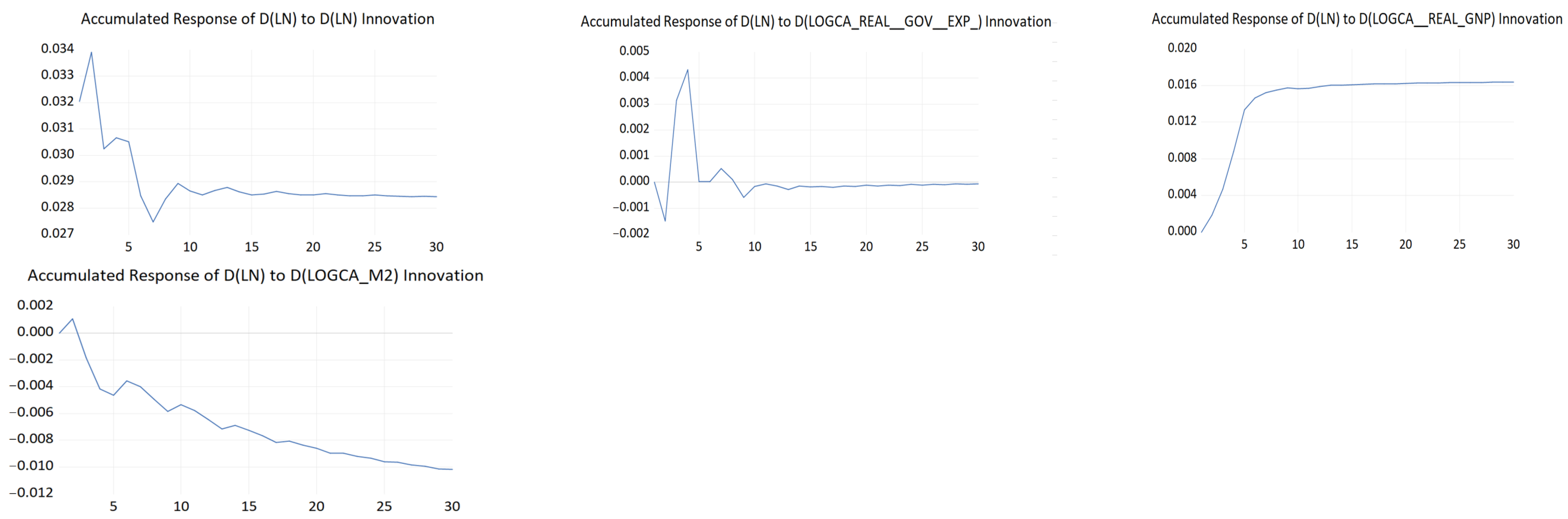
5.3. Impulse Responses

Figure 3 reports the accumulated response of the real and nominal exchange rate of USD/CAD to real and nominal shocks. As witnessed below, the effect of nominal shock on the real USD/CAD quickly dissipates. Nominal shocks have a similar short-lasting effect on the nominal exchange rate. However, the effect of real shocks on the nominal and real exchange rate between the Canadian dollar and U.S. dollar is permanent. Specifically, while we observe a sudden increase for both NER and RER following a real shock, the effect of the real shock overshoots before stabilizing at a higher than before RER. Comparatively, for the NER, the effect of a real shock is a sudden and permanent increase. This suggests that while real shocks have a more long-lasting effect on the nominal and real exchange rate, real shocks tend to lead to an overshooting in the short-run which, however, corrects itself as the market converges to its new long-run equilibrium. This is consistent with the overshooting model of (Dornbusch 1976), where a real shock (e.g., an expansion in demand for output) leads to an increase in demand for money which, in turn, is accompanied by rising interest rates and appreciation of the local currency. This process lingers until output returns to its initial level and price level and exchange rate converge to their new long-run equilibrium. For the nominal exchange rate, real shocks lead to a permanent effect on the nominal exchange rate as observed above. These results are consistent with the findings of (Enders and Lee 1997).

To complement the above analysis, variance decomposition analysis is included to analyze the impact of the real and nominal shocks on both real and nominal exchange rates. For brevity,

Table 5. Variance decomposition (December 1972–December 2023).

Variable	∆RER	∆RER	∆NER	∆NER
Shock	${\in }_{rt}$	${\in }_{nt}$	${\in }_{rt}$	${\in }_{nt}$
1-quarter	98.489	1.511	80.153	19.847
3-quarters	97.589	2.411	80.311	19.689
5-quarters	97.588	2.412	80.311	19.689
7-quarters	97.588	2.412	80.311	19.689
9-quarters	97.588	2.412	80.311	19.689

Note: Table 5 represents the variance decomposition analysis of real and nominal shocks on ∆RER and ∆NER, where ∆RER (∆NER) is the first difference in real (nominal) Canadian dollars per U.S. dollar. ${\in }_{rt}$ ($\in \_nt)$ denotes the real (nominal) shocks. Five quarters are reported. Values are in percentages.

includes only the first five quarters. Consistent with earlier findings from Figure 3, nearly 98% of the variability in real CAD/USD is explained by real shocks, with the remaining 2% from nominal shocks. Similarly, for the nominal CAD/USD, most of the variation (80%) is attributed to real shocks, with the remaining 20% attributed to nominal shocks.

5.4. Real and Nominal Shocks

While the above analysis supports that real and nominal shocks have some discernable impact on the real and nominal USD/CAD, the above analysis does not identify the real and nominal shocks as specific macroeconomic or financial variables. To this effect, we test, in line with the existing literature review, for real shocks, using real government expenditure as a measure of demand shock and real GNP as a supply shock. Money supply (M2) is used as a nominal shock. Impulse response analysis is carried out for each of the shocks, from both Canada and the U.S., on the NER and RER, respectively, with results reported in Figure 4. Differenced log of real government expenditure and differenced log of real GNP were used as real demand and supply shocks, and the nominal log of money supply (M2) was used as a measure of nominal shock. Accumulated responses for the first 30 quarters following the shocks are reported, using the Cholesky (degree of freedom adjusted) decomposition method. All variables were stationary after first-order differencing using the ADF stationary test. Based on maximizing Schwarz, Hannan–Quinn, and Akaike information criteria, one lag and four lags were used in VAR models with U.S. and Canadian shock variables, respectively. A few observations can be made as follows.

First, both U.S. and Canadian money supply have a marginal decrease on both the real and nominal USD/CAD. A slower decay was noticed on the NER following a shock from the Canadian money supply. This is in line with earlier findings that nominal shocks have only a temporary effect on real and nominal exchange rates.

Secondly, supply shocks from real GNP from both countries resulted in a noticeable increase in the real and nominal USD/CAD, before stabilizing at a higher rate after five quarters. This is consistent with earlier findings that real shocks have a permanent effect on both NER and RER. A less significant response was observed on the NER following a shock from the U.S. real GNP, compared to a similar shock from the Canadian real GNP.

Results for the demand-side shocks were mixed. A shock from the Canadian’s real government expenditure resulted in an increase and permanent impact on the RER. This is in line with earlier findings that real shocks cause a permanent effect on RER. Comparatively, a shock from Canada’s real government expenditure also resulted in an increase in the NER, before returning to its original state within five quarters.

Further, a shock from U.S. real government expenditure resulted in lower NER and RER and stabilizing at a new rate after five quarters. Last, but not least, a self-shock resulted in an initial increase in the RER, before falling to stabilize at a lower but positive increase in the RER. This was also the case, for a self-shock in the RER in a system involving Canadian shocks. Comparatively, a self-shock resulted in an increase and permanent impact for NER, in a system involving U.S. shocks. Although not reported here, self-shocks for both NER and RER contributed mostly to the variance decompositions of NER and RER.

6. Concluding Remarks

Deglobalization and decarbonization are important drivers of inflation globally, and more particularly for countries like Canada and the U.S., which are among the leading consumers, producers, and exporters of energy. COVID-19 can be attributed to being a root cause of deglobalization, with a rise in volatility of prices in the last 4 years. After a decade, Canada has begun to witness sustained positive trade balances. Post-COVID-19, both countries yielded real GDP that was increasing at a decreasing rate. While both economies’ wholesale price indices are positively correlated, the nominal exchange rate ranged between 0.7 U.S. dollars (USD) per Canadian dollar (CAD) to 0.8 U.S. during the period 2020–early 2024. Last, but not least, both exports and imports fell in 2023. With this backdrop of events, triggers and facts, this study sheds light on the long-run relationship between the Canadian dollar and the U.S. dollar by (i) showcasing that real shocks affect both the nominal and real exchange rate of USD/CAD and that nominal shocks have only a temporary effect on the USD/CAD; (ii) how real demand and supply shocks impact the nominal and real exchange rate, compared with a shock from nominal factors; (iii) how country-specific (U.S. and Canada) factors affect the USD/CAD in the long run.

Both the U.S. and Canada are strong partners in trade, with their inflation policies (represented by WPIs), economic activity (real GNP) and monetary policy (money supply) measures being strongly positively linked with each other. Both economies’ inflation measures were negatively correlated with the wholesale price ratio, with the higher WPI for Canada, leading to the real rate being lower than the nominal exchange rate. The nominal USD/CAD was strongly negatively correlated with the wholesale price ratio. Although both countries share a strong positive correlation in their money supplies, the money supply from each country had a reduced effect on the wholesale price indices for each country, compared to real government expenditure and real GNP.

Accumulated responses of the real and nominal exchange rates to nominal and real shocks support that the effect from nominal shocks quickly vanishes. Conversely, the effect of real shocks on the nominal and real exchange rate between the Canadian dollar and the U.S. dollar is permanent. Specifically, although we observe a sudden increase for both NER and RER following a real shock, on one hand, the effect of the real shock overshoots before stabilizing at a higher than before RER. On the other hand, the effect of a real shock is a sudden and permanent increase. This result suggests that while real shocks have a more long-lasting effect on the nominal and real exchange rate, real shocks tend to lead to an overshooting in the short-run which, however, corrects itself as the market congregates to its new long-run equilibrium. Most of the variation in real (nominal) USD/CAD is explained by real (nominal) shocks.

Using real government expenditure from Canada and the U.S. as demand factors, both countries’ real GNP as supply factors, and both nations’ nominal money supply as nominal factors, we conduct an analysis of the response of these impulses on the NER and RER. Both the U.S. and Canada’s money supply led to an insignificant decrease in both real and nominal USD/CAD. This is consistent with our earlier findings that nominal shocks have only a temporary effect on the real and nominal exchange rates. Supply shocks from both countries’ real GNPs led to a rise in both real and nominal USD/CAD before stabilizing at a higher rate after five quarters. This is aligned with earlier findings that real shocks have a permanent effect on both NER and RER. A less significant response was detected on the NER following a shock from the U.S.’s real GNP compared to a similar shock from Canada’s real GNP. Findings for demand-side factors were mixed. A shock from Canada’s real government expenditure led to a rise and permanent impact on the RER. This is consistent with earlier findings that real shocks cause a permanent effect on RER. Conversely, a shock from Canada’s real government expenditure also yielded a rise in the NER, before, however, returning to its original state within five quarters. Overall findings support that real shocks have a permanent impact on both the real and nominal USD/CAD exchange rate. Supply-side (real GNP) factors support this conclusive remark more than demand-side (real government expenditure) factors, with nominal money supply barely impacting the long-run relationship between the U.S. dollar and the Canadian dollar.

Overall, the results have some key policy implications which can be summarized as follows. First, policy makers need to be aware that wholesale price indices in Canada are higher than those in the U.S. This is particularly important, as this results in a real exchange rate being lower than its nominal counterpart. Monetary policy actors need to consider this price information when deciding how inflation across borders can affect trade between the two nations. Second, findings support that real factors tend to affect nominal and real exchange rates permanently compared to nominal-based factors such as money supply. It takes roughly five quarters for the effect to stabilize permanently. Specifically, real supply-side factors, in the form of real GNP, tend to advocate for a permanent shock on real and nominal exchange rates. Only Canada’s real government expenditure, as a demand-factor, tends to have a positive long-lasting impact on the USD/CAD. This suggests that this news announcement from Canada plays a critical role in the relationship between the two North American currencies.

This study relies exclusively on a linear VAR model, which fundamentally focuses on obtaining linear relationships among the study variables. While this approach is widely accepted and provides a clear framework for analyzing the impact of real and nominal shocks on exchange rates, it does not account for possible non-linear relationships (Balke 2000). Nonlinear VAR models, such as TVAR, STVAR, MSVAR, BVAR, NN-VAR, and GARCH-VAR, could show additional dynamics that are not captured by a linear model (Granger and Teräsvirta 1993; Krolzig 2013; Banbura et al. 2010; Kuan and Liu 1995; Ling and McAleer 2003).

Future research could benefit from investigating these nonlinear models to determine whether they provide a more nuanced understanding of the relationships between the variables.

Further, in line with the pioneering work of Blanchard and Quah (1988), the vector autoregressive model can also take into account other specific variables such as unemployment and productivity-based factors as shock variables on nominal and real exchange rates. Finally, researchers can also explore how this relationship cognates with other key partner countries as part of the deglobalized world, especially when it comes to the leading foreign currency pairs actively traded globally.

References

1. Adaramola, Anthony Olugbenga, and Oluwabunmi Dada. 2020. Impact of inflation on economic growth: Evidence from Nigeria. Investment Management & Financial Innovations 17: 1–13. [Google Scholar] [CrossRef]
2. Ahmad, Ahmad Hassan, Eric J. Pentecost, and Marie M. Stack. 2023. Foreign aid, debt interest repayments and Dutch disease effects in a real exchange rate model for African countries. Economic Modelling 126: 106434. [Google Scholar] [CrossRef]
3. Arias, Jonas E., Juan F. Rubio-Ramírez, and Daniel F. Waggoner. 2018. Inference based on structural vector autoregressions identified with sign and zero restrictions: Theory and applications. Econometrica 86: 685–720. [Google Scholar] [CrossRef]
4. Avdjiev, Stefan, Wenxin Du, Catherine Koch, and Hyun Song Shin. 2019. The dollar, bank leverage, and deviations from covered interest parity. American Economic Review: Insights 1: 193–208. [Google Scholar] [CrossRef]
5. Baillie, Richard T., and Patrick C. McMahon. 1989. The Foreign Exchange Market: Theory and Econometric Evidence. Cambridge: Cambridge University Press. [Google Scholar]
6. Balke, Nathan S. 2000. Credit and Economic Activity: Credit Regimes and Nonlinear Propagation of Shocks. Review of Economics and Statistics 82: 344–49. [Google Scholar] [CrossRef]
7. Banbura, Marta, Domenico Giannone, and Lucrezia Reichlin. 2010. Large Bayesian Vector Autoregressions. Journal of Applied Econometrics 25: 71–92. [Google Scholar] [CrossRef]
8. Bank for International Settlements. 2022. Triennial Central Bank Survey. Bank of International Settlements. Available online: https://www.bis.org/statistics/rpfx22.htm (accessed on 12 December 2023).
9. Baumeister, Christiane, and James D. Hamilton. 2019. Structural interpretation of vector autoregressions with incomplete identification: Revisiting the role of oil supply and demand shocks. American Economic Review 109: 1873–910. [Google Scholar] [CrossRef]
10. Bénétrix, Agustín S., and Philip R. Lane. 2013. Fiscal shocks and the real exchange rate. International Journal of Central Banking 32: 1–32. Available online: https://www.ijcb.org/journal/ijcb13q3a1.htm (accessed on 12 December 2023).
11. Blanchard, Olivier Jean, and Danny Quah. 1988. The Dynamic Effects of Aggregate Demand and Supply Disturbances (Working Paper No. 2737). National Bureau of Economic Research. Available online: https://www.nber.org/system/files/working_papers/w2737/w2737.pdf (accessed on 12 December 2023).
12. Bouakez, Hafedh, and Aurélien Eyquem. 2015. Government spending, monetary policy, and the real exchange rate. Journal of International Money and Finance 56: 178–201. [Google Scholar] [CrossRef]
13. Bruno, Valentina, and Hyun Song Shin. 2023. Dollar and exports. The Review of Financial Studies 36: 2963–96. [Google Scholar] [CrossRef]
14. Bussière, Matthieu, Guillaume Gaulier, and Walter Steingress. 2020. Global trade flows: Revisiting the exchange rate elasticities. Open Economies Review 31: 25–78. [Google Scholar] [CrossRef]
15. Butt, Shamaila, Muhammad Ramzan, Wing-Keung Wong, Muhammad Ali Chohan, and Suresh Ramakrishnan. 2023. Unlocking the secrets of exchange rate determination in Malaysia: A Game-Changing hybrid model. Heliyon 9: e19140. [Google Scholar] [CrossRef] [PubMed]
16. Canada Action. 2024. Environmental Leadership in Natural Resources. Available online: https://www.canada.ca/en/natural-resources-canada/news/2021/06/canada-in-a-changing-climate-national-issues-report.html (accessed on 10 February 2024).
17. Canada Nuclear Safety Commission. 2023. Regulatory Action. Available online: https://www.cnsc-ccsn.gc.ca/eng/acts-and-regulations/regulatory-action/impala-canada-ltd/ (accessed on 15 March 2024).
18. Canadian Association of Petroleum Producers. n.d. Oil and Natural Gas in Canada. Available online: https://www.capp.ca/energy/canadas-energy-mix/ (accessed on 12 January 2024).
19. Carriero, Andrea, Todd E. Clark, and Massimiliano Marcellino. 2019. Large Bayesian vector autoregressions with stochastic volatility and non-conjugate priors. Journal of Econometrics 212: 137–54. [Google Scholar] [CrossRef]
20. Carrière-Swallow, Yan, Nicolás E. Magud, and Juan F. Yépez. 2021. Exchange rate flexibility, the real exchange rate, and adjustment to terms-of-trade shocks. Review of International Economics 29: 439–83. [Google Scholar] [CrossRef]
21. Charfeddine, Lanouar, and Karim Barkat. 2020. Short-and long-run asymmetric effect of oil prices and oil and gas revenues on the real GDP and economic diversification in oil-dependent economy. Energy Economics 86: 104680. [Google Scholar] [CrossRef]
22. Chicago Mercantile Exchange Group. 2024. Crude Oil Futures and Options. CME Group. Available online: https://www.cmegroup.com/markets/energy/crude-oil/light-sweet-crude.html (accessed on 21 March 2024).
23. Demir, Firat, and Arslan Razmi. 2022. The real exchange rate and development theory, evidence, issues and challenges. Journal of Economic Surveys 36: 386–428. [Google Scholar] [CrossRef]
24. Dibooglu, Selahattin, and Walter Enders. 1995. Multiple cointegrating vectors and structural economic models: An application to the French Franc/US Dollar exchange rate. Southern Economic Journal 61: 1098–116. [Google Scholar] [CrossRef]
25. Dogru, Tarik, Cem Isik, and Ercan Sirakaya-Turk. 2019. The balance of trade and exchange rates: Theory and contemporary evidence from tourism. Tourism Management 74: 12–23. [Google Scholar] [CrossRef]
26. Dornbusch, Rudiger. 1976. Expectations and exchange rate dynamics. Journal of political Economy 84: 1161–76. [Google Scholar] [CrossRef]
27. Eichenbaum, Martin, Benjamin K. Johannsen, and Sergio Rebelo. 2021. Monetary policy and the predictability of nominal exchange rates. The Review of Economic Studies 88: 192–228. [Google Scholar] [CrossRef]
28. Enders, Walter. 2014. Applied Econometric Time Series. New York: Wiley. [Google Scholar]
29. Enders, Walter, and Bong-Soo Lee. 1997. Accounting for real and nominal exchange rate movements in the post-Bretton Woods period. Journal of International Money and Finance 16: 233–54. [Google Scholar] [CrossRef]
30. Evans, George W. 1987. Output and Unemployment Dynamics in the United States: 1950–1985. London: London School of Economics. [Google Scholar]
31. Factset. 2024. Investment Research. Available online: https://www.factset.com/solutions/investment-research (accessed on 16 January 2024).
32. Fisher, Lance A., and Hyeon-Seung Huh. 2002. Real exchange rates, trade balances and nominal shocks: Evidence for the G-7. Journal of International Money and Finance 21: 497–518. [Google Scholar] [CrossRef]
33. Frankel, Jeffrey A., and Andrew K. Rose. 1995. Empirical research on nominal exchange rates. Handbook of International Economics 3: 1689–729. [Google Scholar] [CrossRef]
34. Frenkel, Jacob A. 1976. Inflation and the Formation of Expectations. Journal of Monetary Economics 1: 403–21. [Google Scholar] [CrossRef]
35. Global Affairs Canada. 2020. The Canada-United States-Mexico Agreement: Economic Impact Assessment. Available online: https://www.international.gc.ca/trade-commerce/assets/pdfs/agreements-accords/cusma-aceum/cusma-impact-repercussion-eng.pdf (accessed on 19 July 2024).
36. Government of Canada. 2024. Coal Facts. Available online: https://natural-resources.canada.ca/our-natural-resources/minerals-mining/mining-data-statistics-and-analysis/minerals-metals-facts/coal-facts/20071 (accessed on 14 April 2024).
37. Granger, Clive W. J., and Timo Teräsvirta. 1993. Modeling Nonlinear Economic Relationships. Oxford: Oxford University Press. [Google Scholar]
38. Greenwood, Robin, Samuel Hanson, Jeremy C. Stein, and Adi Sunderam. 2023. A quantity-driven theory of term premia and exchange rates. The Quarterly Journal of Economics 138: 2327–89. [Google Scholar] [CrossRef]
39. Gründler, Daniel, Eric Mayer, and Johann Scharler. 2023. Monetary policy announcements, information shocks, and exchange rate dynamics. Open Economies Review 34: 341–69. [Google Scholar] [CrossRef]
40. Gurrib, Ikhlaas, and Firuz Kamalov. 2019. The implementation of an adjusted relative strength index model in foreign currency and energy markets of emerging and developed economies. Macroeconomics and Finance in Emerging Market Economies 12: 105–23. [Google Scholar] [CrossRef]
41. Gurrib, Ikhlaas, and Firuz Kamalov. 2022. Predicting bitcoin price movements using sentiment analysis: A machine learning approach. Studies in Economics and Finance 39: 347–64. [Google Scholar] [CrossRef]
42. Gurrib, Ikhlaas, Firuz Kamalov, Olga Starkova, Adham Makki, Anita Mirchandani, and Namrata Gupta. 2023. Performance of Equity Investments in Sustainable Environmental Markets. Sustainability 15: 7453. [Google Scholar] [CrossRef]
43. Gürkaynak, Refet S., A. Hakan Kara, Burçin Kısacıkoğlu, and Sang Seok Lee. 2021. Monetary policy surprises and exchange rate behavior. Journal of International Economics 130: 103443. [Google Scholar] [CrossRef]
44. Hanif, Waqas, Walid Mensi, Mohammad Alomari, and Jorge Miguel Andraz. 2023. Downside and upside risk spillovers between precious metals and currency markets: Evidence from before and during the COVID-19 crisis. Resources Policy 81: 103350. [Google Scholar] [CrossRef]
45. Huang, Chunhua. 2020. Research on the linkage relationship between different levels of money supply and economic growth based on VAR model. Paper presented at 2020 2nd International Conference on Economic Management and Model Engineering (ICEMME), Chongqing, China, 20–22 November. [Google Scholar]
46. International Energy Agency. 2022. Canada 2022: Energy Policy Review. February 26. Available online: https://www.iea.org/reports/canada-2022 (accessed on 2 January 2024).
47. Ji, Qiang, Syed Jawad Hussain Shahzad, Elie Bouri, and Muhammad Tahir Suleman. 2020. Dynamic structural impacts of oil shocks on exchange rates: Lessons to learn. Journal of Economic Structures 9: 1–19. [Google Scholar] [CrossRef]
48. Jia, Yanjing, Zhiliang Dong, and Haigang An. 2023. Study of the modal evolution of the causal relationship between crude oil, gold, and dollar price series. International Journal of Energy Research 2023: 7947434. [Google Scholar] [CrossRef]
49. Kamalov, Firuz, and Ikhlaas Gurrib. 2022. Machine learning-based forecasting of significant daily returns in foreign exchange markets. International Journal of Business Intelligence and Data Mining 21: 465–83. [Google Scholar] [CrossRef]
50. Kamalov, Firuz, Ikhlaas Gurrib, and Khairan Rajab. 2021. Financial forecasting with machine learning: Price vs. return. Journal of Computer Science 17: 251–64. [Google Scholar] [CrossRef]
51. Kelesbayev, Dinmukhamed, Kundyz Myrzabekkyzy, Artur Bolganbayev, and Sabit Baimaganbetov. 2022. The impact of oil prices on the stock market and real exchange rate: The case of Kazakhstan. International Journal of Energy Economics and Policy 12: 163–68. [Google Scholar] [CrossRef]
52. Kilian, Lutz. 2013. Structural vector autoregressions. In Handbook of Research Methods and Applications in Empirical Macroeconomics. Cheltenham: Edward Elgar Publishing, pp. 515–54. [Google Scholar]
53. Kilian, Lutz, and Helmut Lütkepohl. 2017. Structural Vector Autoregressive Analysis. Cambridge: Cambridge University Press. [Google Scholar]
54. Kim, Jin-Ock, and Walter Enders. 1991. Real and monetary causes of real exchange rate movements in the Pacific Rim. Southern Economic Journal 57: 1061–70. [Google Scholar] [CrossRef]
55. King, Robert G., and Mark W. Watson. 1992. Testing Long Run Neutrality (September 1992). NBER Working Paper No. w4156. Available online: https://ssrn.com/abstract=226809 (accessed on 15 December 2023).
56. Krolzig, Hans-Martin. 2013. Markov-Switching Vector Autoregressions: Modelling, Statistical Inference, and Application to Business Cycle Analysis. Berlin/Heidelberg: Springer Science & Business Media, vol. 454. [Google Scholar]
57. Kuan, Chung-Ming, and Tung Liu. 1995. Forecasting exchange rates using feedforward and recurrent neural networks. Journal of Applied Econometrics 10: 347–64. [Google Scholar] [CrossRef]
58. Lane, Philip R., and Gian Maria Milesi-Ferretti. 2007. The external wealth of nations mark II: Revised and extended estimates of foreign assets and liabilities, 1970–2004. Journal of international Economics 73: 223–50. [Google Scholar] [CrossRef]
59. Lavoie, Marc, and Mario Seccareccia. 2006. The Bank of Canada and the modern view of central banking. International Journal of Political Economy 35: 44–61. [Google Scholar] [CrossRef]
60. Lee, Chien-Chiang, and Jafar Hussain. 2023. An assessment of socioeconomic indicators and energy consumption by considering green financing. Resources Policy 81: 103374. [Google Scholar] [CrossRef]
61. Ling, Shiqing, and Michael McAleer. 2003. Asymptotic theory for a vector ARMA-GARCH model. Econometric Theory 19: 280–310. [Google Scholar] [CrossRef]
62. Liu, Donghui, Lingjie Meng, and Yudong Wang. 2020. Oil price shocks and Chinese economy revisited: New evidence from SVAR model with sign restrictions. International Review of Economics & Finance 69: 20–32. [Google Scholar]
63. Malik, Farooq, and Zaghum Umar. 2019. Dynamic connectedness of oil price shocks and exchange rates. Energy Economics 84: 104501. [Google Scholar] [CrossRef]
64. Mao, Yuntao, Ziwei Chen, Siyuan Liu, and Yanfeng Li. 2024. Unveiling the potential: Exploring the predictability of complex exchange rate trends. Engineering Applications of Artificial Intelligence 133: 108112. [Google Scholar] [CrossRef]
65. Meese, Richard A., and Kenneth Rogoff. 1983. Empirical exchange rate models of the seventies: Do they fit out of sample? Journal of International Economics 14: 3–24. [Google Scholar] [CrossRef]
66. Moulle-Berteaux, Cyril. 2023. Global Multi-Asset Viewpoint: The Five Forces of Secular Inflation. Morgan Stanley Investment Management. Available online: https://www.morganstanley.com/im/publication/insights/articles/article_thefiveforcesofsecularinflation.pdf (accessed on 15 December 2023).
67. Mussa, Michael. 1976. Adaptive and regressive expectations in a rational model of the inflationary process. Journal of Monetary Economics 1: 423–42. [Google Scholar] [CrossRef]
68. Nakatani, Ryota. 2017. The effects of productivity shocks, financial shocks, and monetary policy on exchange rates: An application of the currency crisis model and implications for emerging market crises. Emerging Markets Finance and Trade 53: 2545–61. [Google Scholar] [CrossRef]
69. Natural Resources Canada. 2023. Energy Factbook 2023–24. Available online: https://energy-information.canada.ca/sites/default/files/2023-10/energy-factbook-2023-2024.pdf (accessed on 16 February 2024).
70. Plotnick, Alan R. 1963. Oil Imports: Protectionism vs. National Security. Challenge 11: 28–32. [Google Scholar] [CrossRef]
71. Sarangi, Pradeepta Kumar, Muskaan Chawla, Pinaki Ghosh, Sunny Singh, and P. K. Singh. 2022. FOREX trend analysis using machine learning techniques: INR vs. USD currency exchange rate using ANN-GA hybrid approach. Materials Today: Proceedings 49: 3170–76. [Google Scholar] [CrossRef]
72. Sarno, Lucio, and Mark P. Taylor. 2001. Official intervention in the foreign exchange market: Is it effective and, if so, how does it work? Journal of Economic Literature 39: 839–68. [Google Scholar] [CrossRef]
73. Sánchez, Juan José García. 2023. American Protectionism: Can It Work? Epicenter At the Heart of Research and Ideas, Harvard University. August 16. Available online: https://epicenter.wcfia.harvard.edu/blog/american-protectionism-can-it-work (accessed on 23 May 2024).
74. Sims, Christopher A. 1980. Macroeconomics and reality. Econometrica: Journal of the Econometric Society 48: 1–48. [Google Scholar] [CrossRef]
75. Sokhanvar, Amin, and Chien-Chiang Lee. 2023. How do energy price hikes affect exchange rates during the war in Ukraine? Empirical Economics 64: 2151–64. [Google Scholar] [CrossRef]
76. Sokhanvar, Amin, Serhan Çiftçioğlu, and Chien-Chiang Lee. 2023. The effect of energy price shocks on commodity currencies during the war in Ukraine. Resources Policy 82: 103571. [Google Scholar] [CrossRef]
77. Suhendra, Indra, and Cep Jandi Anwar. 2022. The response of asset prices to monetary policy shock in Indonesia: A structural VAR approach. Banks and Bank Systems 17: 104–14. [Google Scholar] [CrossRef]
78. Tan, Eu Chye, Chor Foon Tang, and Rupah Devi Palaniandi. 2022. What could cause a country’s GNP to be greater than its GDP? The Singapore Economic Review 67: 557–66. [Google Scholar] [CrossRef]
79. Yilmazkuday, Hakan. 2023. COVID-19 effects on the S&P 500 index. Applied Economics Letters 30: 7–13. [Google Scholar]
80. Yıldız, Bünyamin Fuat, Siamand Hesami, Husam Rjoub, and Wing-Keung Wong. 2021. Interpretation of oil price shocks on macroeconomic aggregates of South Africa: Evidence from SVAR. The Journal of Contemporary Issues in Business and Government 27: 279–87. [Google Scholar]
81. Youssef, Manel, and Khaled Mokni. 2020. Modeling the relationship between oil and USD exchange rates: Evidence from a regime-switching-quantile regression approach. Journal of Multinational Financial Management 55: 100625. [Google Scholar] [CrossRef]
82. Zhou, Su. 1995. The response of real exchange rates to various economic shocks. Southern Economic Journal 61: 936–54. [Google Scholar] [CrossRef]
Figure 1. Presence of Canadian dollar and USD in foreign currency trades. Note: Figure 1 reports the average daily turnover of Over-The-Counter (OTC) foreign exchange instruments for the Canadian dollar (CAD) and U.S. dollar (USD) for 2001–2022. Source: Bank for International Settlements (2022).
Jrfm 17 00411 g001
Figure 2. NER and RER for Canada (December 1972–December 2023). Note: Figure 2 displays the nominal exchange rates (NER) and real exchange rates (RER) for Canada, using quarterly wholesale price ratios for the period December 1972–December 2023.
Jrfm 17 00411 g002
Figure 3. Response of RER and NER to nominal and real shocks. Note: Figure 3 displays the accumulated response of real USD/CAD (RER) and nominal USD/CAD (NER) to real shocks (shock 1) and nominal shocks (shock 2).
Jrfm 17 00411 g003
Figure 4. Impulse responses of real and nominal shocks from the U.S. and Canada on NER and RER (December 1972–December 2023). Note: Figure 4 displays the response of the real and nominal USD/CAD to real and nominal shocks from Canada and the U.S. Differenced logs of real government expenditure and differenced logs of real GNP were used as real demand and supply shocks, and money supply (M2) was used as a measure of nominal shock. Accumulated responses for 30 first quarters following the shocks are reported, using Cholesky (degree of adjusted) decomposition. All variables were stationary after first-order differencing using the ADF stationary test. Based on maximizing Schwarz, Hannan–Quinn, and Akaike information criteria, 1 lag and 4 lags were used in VAR models with U.S. and Canadian shock variables, respectively. The period of study is December 1972–December 2023.
Jrfm 17 00411 g004aJrfm 17 00411 g004b