Abstract
This study aims to answer the question about the interactions between “investors’ fear”, two factors proposed by Fama & French, the Carhart momentum factor, andthe risk premium, and how these interactions were affected by two financial crises, the Dot-Com and Sub-Prime crises. This paper is the first empirical study that considers the effects of these financial crises. It is of critical importance as it changes the specificity of the empirical models for different periods, significantly affecting the results compared to previous research work. The main findings include a general negative change in fear over all of the sub-periods. Secondly, no consistent positive trend was observed in any of the risk premiums over time. After each crisis, the relationships between the endogenous variables had significant changes. More specifically, investors’ fear, on the first day of the week, appears to be systematically higher across all sub-periods except during the Sub-Prime crisis. Finally, after the Sub-Prime financial crisis, there is an almost complete loss of the explanatory power of the VAR models. Although fear does not seem to affect risk premiums or momentum, it was nevertheless found that the results are sensitive to the specification of the models.
1. Introduction
Merton (1980) made a significant contribution by showing that market returns, or the risk premium E(Rm-rf), are positively correlated with risk. This means that as the volatility of stock returns increases, so does the desired return for investors, resulting in an increase in the risk premium. Building on this, Fama and French (1993) introduced two additional factors—size (SMB) and value (HML)—to further explain changes in risk aversion. Lastly, Carhart (1997) added the momentum factor, proving that it, along with volatility and the Fama–French factors, aids in understanding the movements of the market premium. The VIX volatility index, created in 1993 by the Chicago Stock Ex-change, measures the anticipated volatility of the S&P 500 index of the American Money Market. It does so by calculating the implied variance from options prices on the S&P 500 index. With its inverse relationship to S&P 500 returns, coupled with its predictive nature, it is natural to view the VIX as a reflection of investor fear (Durand et al. 2011). The VIX expected volatility index has a direct impact on the market risk premium, as market returns are not constant but rather fluctuate over time. Typically, the measure of uncertainty is determined by the variation or expected variation in returns. This premium incentivizes investors to take on additional risk, as a higher return is offered. As uncertainty rises and the potential spread between market returns and the risk-free rate widens, investors are more inclined to invest. Otherwise, they would not be willing to take on extra uncertainty.
This study focuses on the relationship and impact between “investors’ fear”, two factors described by Fama and French (1993), and the Carhart (1997) momentum factor on the risk premium. The purpose of this research is to determine which variable influences one another, the direction of their influence, and if a causal relationship exists between them (as analysed by Granger). The study also investigates the duration of these interactions.
Our analysis concentrates on two major crisis periods. The time period of the COVID-19 crisis has also been included in our analysis, but as we have not passed enough time after the crisis, the crises which are studied in the form of “pre” and “post” are the first two mentioned. The first was triggered by the collapse of the Dot-Com bubble, which led to an economic recession. This was followed by a second period of recession caused by the Sub-Prime mortgage bubble bursting. In both cases, the initial financial boom turned out to be unsustainable and resulted in a dramatic collapse, sending shockwaves through the stock markets. Consequently, economic activity decreased and contracted. More specifically, this research focuses on how these interrelationships and interactions have evolved from January 1991 to February 2024, taking into consideration the two major financial crises that the American economy experienced during this period: the Dot-Com bubble and the Sub-Prime mortgage crisis which led to a global recession.
By examining five variables (the size factor, the value factor, the momentum factor, the risk factor, and the VIX index), using Vector Autoregressive (VAR) estimates and impulse response analysis results, we aim to gain insight into the effects of these crises on the relationship between “investors’ fear”, Fama and French’s factors, and the Carhart momentum factor.
The paper is organized as follows: In the next section, it is presented a literature review that focuses on the effects of the financial crises of Dot-Com and Sub-Prime and the applications of the Fama–French model in different economic scenarios. Furthermore, two hypotheses are examined and the expected outcomes for the upcoming empirical tests are presented. The research methodology is explained in detail, covering important elements such as sample selection and data coding. Moreover, we present and carefully analyse our empirical findings, concluding with a comprehensive discussion.
2. Literature Review and Hypothesis Development
This section presents a synopsis of the literature relative to the five endogenous variables examined in this study (the size factor, the value factor, the momentum factor, the risk factor, and the VIX index) and the research hypotheses developed.
2.1. The Size Factor
The “size factor” (SMB) indicates that smaller firms usually provide higher returns than larger firms (Fama and French 1993). This variable is a key indicator as to whether a smaller-cap stock has the potential to generate higher returns compared to a larger-cap stock. According to Roll (1981), the reason behind the existence of the premium can be attributed to difficulties in measuring risks and evaluating performance. Similarly, Shumway (1997) proposes that data and calculation issues are responsible for the observed pattern of the size premium. Additionally, behavioural perspectives have been put forth to explain this phenomenon. For instance, Kumar and Lee (2003) suggest that changes in investor sentiments play a significant role on the size premium trend. However, Durand et al. (2007) show that in the Australian market, variations in the size premium are closely linked to investors’ emotional reactions and tendencies to over- or under-react.
2.2. The Value Factor
The “value factor” (High Minus Low, or HML) states that stocks with a high book-to-financial value offer higher returns than low-value stocks (Fama and French 1993). The value factor indicates that undervalued stocks, known as “value stocks”, with a high market-to-book value ratio provide higher returns than overvalued stocks, known as “growth stocks”, with a lower market-to-book value ratio (Fama and French 1993). They incorporated the value factor (HML) into Merton’s model. Within this factor, value is determined by stocks with a high book-to-market value and growth by stocks with a low ratio of this value, depending on market capitalization. The difference in returns between these two types of stocks is usually mentioned as the “value-to-growth premium”. Research by Rozeff and Zaman (1998) indicates that market participants seem to exploit this premium by selling undervalued stocks and buying overvalued ones, thus changing their returns. According to La Porta et al. (1997), value premium is attributed to the overreaction of investors to the flow of information concerning earnings, which drives stocks away from their correct values. However, research by Houge and Lughran (2006) finds no evidence in favour of a value-to-growth premium, while other studies, such as Vassalou and Xing (2004) and Petkova and Zhang (2005) argue that HML reflects the expectations of investors about the possibility of bankruptcy and future financial well-being.
2.3. The Momentum Factor
The “momentum factor”, as analysed by Carhart (1997), attributes the upward or downward movement of stocks to the overreaction phenomenon of financial markets. The factor can be measured as the difference between the returns of the highest-returning stocks and the lowest-returning stocks over a period of 2 to 12 months prior. Jegadeesh and Titman (1993) examine the momentum factor in a portfolio that includes strongly bullish stocks in a long position or weak stock returns in the short position. Agarwal and Taffler (2008) state that the momentum effect is a consequence of the financial distress factor, combining its relationship with the HML and SMB factors. Barberis et al. (1998) highlight the relationship of momentum with the degree of underreaction to new information in a short-term period. Grinblatt and Han (2005) point out that investors who have not experienced losses or gains in their portfolios are more wary of selling unprofitable than profitable stocks. Campello et al. (2008) find a significant effect of momentum on the size premium and stock value, while Durand et al. (2011) focus on the interactions between HML, SMB, and momentum factors in the period of 1996–2007, highlighting the importance of the latter in the evolution of returns.
2.4. The Risk Factor
Extending the research field globally, many researchers have analysed the contribution of Fama–French model risk factors to international stock market spillovers and have studied the effects of risk factors, including momentum, on stock returns using the Bisnis-27 Index. The research results indicated that investors should consider risk premium, company size, and stock dynamics when they make investment decisions to achieve higher returns. The findings across various studies strongly emphasize the need for a discerning approach in making investment choices. This entails weighing not just risk factors and momentum, but also the symbiotic relationship between financial success and the tone of communication from a CEO. By considering these factors, investors can make informed decisions, fortified by a well-rounded understanding gleaned from these studies. This, in turn, elevates the overall discourse surrounding financial matters, imparting valuable insights into the complexities of risk assessment and performance evaluation (Mlawu et al. 2023). Adding another layer to this narrative, the role of CEO social capital emerges as a critical factor in shaping equity valuation dynamics (Luehlfing et al. 2023). In the same direction, Basdekis et al. (2023b) highlight the role of women executives in firms’ performance. Furthermore, Luehlfing et al. (2023) examine the complex relationship between tax avoidance and corporate risk tolerance, highlighting the crucial impact of corporate governance mechanisms. Researchers have examined the dynamic applications of the Fama–French model, investigating its utility across various economic conditions. Horvath and Wang (2021) conducted a thorough examination of the model’s performance during the unprecedented COVID-19 crisis, while Horvath and Wang (2021) explored its relevance in the US REIT market, taking into account factors such as financial distress and liquidity crises spanning from 2001 to 2020. Kostin et al. (2022) further evaluated the model’s validity in times of crisis, utilizing a select group of energy-sector companies during the COVID-19 pandemic as a case study. Basdekis et al. (2023a) examined the effect of ECB’s unconventional monetary policy on firms’ performance during the global financial crisis. In addition, Konstantinov and Fabozzi (2021) focused on the EMU bond market, while Chaudhary et al. (2020) examined the impact of COVID-19 on volatility in international stock markets. These comprehensive investigations contribute to a nuanced understanding of the robustness and applicability of the Fama–French model in diverse financial landscapes. These studies enhance and enrich our overall understanding of this model. Guo et al. (2022) extended their research to include the Chinese stock market in the post-financial crisis era. Finally, Viippola (2020) examined the impact of corporate social responsibility on stock returns during the challenging COVID-19 crisis.
Based on the above, the relationship between risk-neutral momentum and the autocorrelation of returns leads to the conclusion that risk-neutral momentum can be a new perspective for risk management. Despite the existence of studies focusing on the relationship between risk premium, Fama–French factors, momentum, and investors’ fear, limited research is available in those which include not only the factors mentioned above but also the effect of these two financial crises on previous interactions.
2.5. The VIX Index
The VIX index, also known as the “fear index”, reflects market expectations about future uncertainty and risk, affecting market performance. The VIX index is an important tool in the field of financial analysis. Through the VIX, investors can track market expectations concerning future uncertainty and risk. At the same time, this index links Merton’s theory of the positive relationship between return and risk with the Fama–French factors, including value, size, and momentum, as factors that affect the investment performance. Therefore, the VIX is also an important measure that combines market predictability with risk assessment, thus providing meaningful information for investors and analysts. The VIX represents investors’ expectations about the future volatility of the US stock market, S&P 500. When the VIX rises, it indicates that there is increased fear in the markets as investors expect increased volatility. Respectively, the retreating VIX indicates investors’ prosperity and confidence. In the field of market analysis, Merton’s theory states that market performance is positively related to risk, where increased risk requires higher returns. The Fama–French factors add value, company size, and momentum as additional investment performance factors. Also, the VIX reflects the uncertainty of the market, affecting the risk premium. When investors are worried due to increased fear, they demand higher profits to withstand this extra risk. Finally, the VIX is also an indicative of future market growth based on changes in expected volatility.
As evidenced, there is a substantial gap in research on the relationships between risk premium, Fama–French factors, momentum, and investor fear. Although Durand et al. (2011) stands as an exception, their research on these effects does not fully explore the causality behind them. As a result, the understanding of how these variables interact remains insufficient. The central aim of this paper is to bridge and alleviate this research gap. Therefore, the research hypotheses that are pursued are presented below:
H1:
Interactions between the endogenous variables did not remain constant over time and are different before and after each crisis.
Because of the importance of the Dot-Com and the Sub-Prime crises, it is expected that relationships between the variables largely change. Every crisis changes investors’ behaviour because of the changes in the regulatory framework. Furthermore, the interactions between the factors will also be examined, based on the findings of Durand et al. (2011).
H2:
There are interactions between the endogenous variables in all sub-periods.
The endogenous variables examined in this paper are the size factor, the value factor, the momentum factor, the risk premium, and the VIX index.
3. Data Presentation
The data set of the research consists of five variables, for which they have collected data in the form of a time series, over a period of twenty years. The data period of the study is from January 1994 to February 2024 and there are a total of 8353 daily measurements of the five endogenous variables. This period of time contains two financial crises (the Dot-Com and Sub-Prime crises) and a health crisis (COVID-19 pandemic crisis) which clearly also had financial dimensions. Regarding the period of the COVID-19 crisis, as we have not passed enough time after the crisis, we are not able to study it in terms of pre- or post-crisis. Regarding the fractioning of the whole time period, in order not to have elements of opportunism and arbitrariness in the methodology, it is important to have a definition from an outside third source to define recessions. This is the main utility of using the NBER. Based on the NBER we have divided the examined period from 04/1991 to 12/2015 into five sub-periods, according to the NBER’s calendar of recessions of the global economy. Initially, the two crisis periods include the Dot-Com and Sub-Prime crises; more specifically, the periods from March 2001 to October 2001 and from January 2008 to May 2009, respectively. Subsequently, we defined the periods of each, which are presented in Table 1 below. The fact that the number of observations varies significantly from one sub-period to another is necessitated by reality itself and the length of the time periods.

Table 1.
Sub-periods of the sample.
Table 2 below contains a list of variables as they appear in EViews, matching them with those described in the previous section.
Table 2.
Endogenous variables.
Table 3 below indicates the descriptive statistics for all five variables in all sub-periods. In Table 3, it is evident that the Jarque–Bera statistic is very large for all the variables. This statistic tests the following null hypothesis:
Table 3.
Descriptive statistics of the variables.
H0:
The variable follows a normal distribution, for each variable.
For a significance level of 5% (p-value ≡ “probability” ≈ 0 < 0.05), we reject the null hypothesis of the normal distribution. Thus, none of our endogenous variables in any sub-period appears to be normally distributed. We consider that Bonferroni correction for all the Jarque–Bera tests is not needed, as all p-values are close to 0.
For the market premium, we observe that its average value (“Mean”) is negative during the periods of the two crises. This result is justified by the fact that during the periods of crises, market returns are lower—negative in most of them—than the risk-free interest rate. As for the volatility of the premium (“Std. Dev.”), we observe that during the periods of the crises there is an increase compared to the periods before and after the two crises. In times of crisis, the returns on risky bonds are mainly negative, while their volatility rises due to an increase in risk. In fact, during the Sub-Prime crisis the volatility of the premium increased to a greater extent in relation to the Dot-Com crisis, which is a major indication of the peculiarity of the Sub-Prime crisis. Concerning the symmetry (“Skewness”) of the premium, we notice that it is quite close to 0; the distribution of the premium can be characterized as symmetrical. The kurtosis (“Kurtosis”) of the premium is of great interest. The pre-Dot-Com premium curvature was almost twice as high as during the Dot-Com crisis and has remained low in the post-Dot-Com period. Briefly, the premium had fat tails (a higher probability of extreme prices) while these largely weakened from the Dot-Com onwards. In all sub-periods after the Dot-Com crisis the kurtosis is above 5, so there are fat tails, but not as they were mentioned before the crisis in 2001. This phenomenon of hyperreaction of the markets has been widely studied in the empirical literature (La Porta et al. 1997).
The “size premium” (SMB) shows whether companies with smaller capitalizations outperform those with larger capitalizations. The descriptive statistics of this variable are also in Table 3. For the average price (“Mean”) of the size premium, we observe that it is positive in almost all periods, except for the one before the Dot-Com crisis, while it has a very small value close to zero. This means that, on average, the size premium did not exist for most of the 1990s although Campello et al. (2008) did not find anything similar. Of course, in their analysis, they had not divided the time horizon into sub-periods. The volatility of SMB (“Std. Dev.”) is small (<0.9) in all sub-periods and does not appear to be affected by either shock, as was the case with the market premium. The skewness of the SMB remains consistently negative over time, indicating that the largest number of observations are above the mean value which we have seen to be low. From the latter we can conclude that there is indeed a positive size premium, but this is more evident from 2000 onwards. The negative symmetry of course recedes (in absolute value) closer to zero during the period of the Sub-Prime crisis.
Finally, the kurtosis (“Kurtosis”) is large until the Dot-Com crisis and during the Sub-Prime crisis, indicative that there are fat tails in those periods, while before and after the Sub-Prime crisis it is too low. Thick tails in the kurtosis mean that there are large outliers in the difference in returns between small- and large-cap companies; this was the case up until the Dot-Com crisis and happened again in the recession that followed the Sub-Prime crisis.
The “value-to-growth premium” (HML), i.e., the difference in returns between listed companies with a high book-to-market ratio (value), minus the returns of those with a low book-to-market value (growth) ratio. From Table 3, we observe that the mean (“Mean”) is positive in most periods except during the Sub-Prime crisis when it became negative. This means that during this crisis, growth stocks outperformed, on average, the returns of value stocks. This means that investors have turned to growth stocks, which should not surprise us, as expansionary US monetary policy has triggered the rise in stock prices by showing investors that growth stocks have consistently deviated from their book value without reason to “be corrected”. The volatility (“Std. Dev.”) of the value-to-growth premium also remains chronically low, but increases considerably during periods of crises. Especially in the Sub-Prime crisis, where it almost tripled from the pre-crisis (and post-Dot-Com) period, although the pre-Sub-Prime period had the lowest volatility for HML. Skewness shows a somewhat strange behaviour: it is negative only in the Dot-Com period and before the Sub-Prime, while in the other periods it is positive. For kurtosis (“Kurtosis”), HML shows very fat tails (three times the kurtosis of the normal distribution) until the Dot-Com crisis, when it halves and remains low. Low, but always greater than the kurtosis of the normal distribution, so there are thick tails even after Dot-Com in the premium of value minus growth stocks, but to a much lesser extent.
For both SMB and HML, we observe that there is a countercyclicality only during the Dot-Com crisis period, while for the next crisis period (that of Sub-Prime) there is no countercyclicality in these two premiums. According to the findings of Campello et al. (2008), we expect countercyclical behaviour of SMB and HML (increasing in times of crisis), which occurs in the Dot-Com crisis, but it seems that this countercyclicality ceases to exist in the Sub-Prime crisis.
The “momentum factor” (WML) expresses whether stocks with high returns continue to have high returns or stocks with low returns continue to have low returns; that is, there is a maintenance of momentum in the stock returns of a market. The average value (“Mean”) of momentum is positive in all sub-periods except during the Sub-Prime crisis when it became negative. This means that stocks that previously (2 to 12 months before) had negative returns realized larger and/or positive returns. This is reasonable for a period of crisis, especially during Sub-Prime, as the peculiar monetary easing measures supported the positive development in the returns of most stocks. In other words, the stocks that fell due to the crisis, then recovered due to the passing of the main phase of the crisis and due to the monetary easing. In Dot-Com this did not appear, perhaps because the duration of the crisis was clearly shorter. As for the volatility (“Std. Dev.”) of the momentum factor, it increased—almost doubled—in the two periods of crises compared to the periods of “normality”, so we observe an increase in the volatility of momentum when the economic cycle recedes. For skewness and kurtosis, their behaviour changed greatly from the Dot-Com crisis onwards: in the pre-Dot-Com period, the symmetry was much lower (more negative); since then, the kurtosis was 19.03, which is more than three times the kurtosis in the rest of the period. Essentially, the most likely values of the momentum were quite a bit larger than its mean value, but the existence of such extremely thick tails may indicate that the pre-Dot-Com momentum distribution was quite broad after all. The broad distribution of momentum suggests that, perhaps finally, stocks have begun to show persistence in their returns since the beginning of the 21st century and beyond.
Based on the results from Table 3 below, there is a consistent pattern in the fluctuations of the “VIX” index, which measures the fear of investors. In comparison to the remaining factors and the market premium, the changes in the VIX index are smoother. The average percentage changes in the VIX index remained negative throughout all periods, indicating that investors have a tendency towards complacency. Moreover, the volatility of investors’ fear remained constant over time, with a slight increase noted only after the Sub-Prime crisis. Overall, the results suggest that investors are more likely to be complacent than scared, and their levels of fear do not show significant fluctuations even during times of crises. The analysis indicates that the skewness of the VIX, or the change in fear, is typically positive across all time periods. However, during the Sub-Prime crisis, this trend is reversed and becomes negative. This suggests that during this crisis, investor fear manifested itself predominantly in positive changes, surpassing the average level. It’s understandable that a crisis of this magnitude, especially with its prolonged duration, would induce a heightened sense of fear among investors. However, even during this challenging time, the low kurtosis values indicate that extreme changes in fear were not prevalent.
4. Results and Discussion
Τhis section is organized as follows: First, the correlations of the variables are discussed. The appropriate stationarity tests and causality tests follow. Finally, the Vector Autoregression (VAR) estimates accompanied with the impulse responses results are presented, and critically discussed against prior relative studies.
4.1. Correlations between Variables
Table 4 below presents the correlations between our five endogenous variables for each of the five sub-periods. To begin with, it is expected that investors’ fear is negatively and strongly related to market returns: when investors start to fear, the market should go down, and vice versa. We, therefore, observe in Table 4 that there is a negative correlation between DVIX and market premium—in all periods. In the next subsection we will examine Granger causality to determine the direction of this correlation: does fear drive the market down, or does fear increase when the market starts to go down? Furthermore, in Table 4 it is evident that the value-to-growth premium is quite—but negatively—correlated with the market premium. This correlation declines and, finally, from Sub-Prime onwards it becomes positive. Given how the value-to-growth premium is calculated, we can say that this applies until the Sub-Prime crisis growth stocks (whose returns are in the denominator of the HML) are more favoured by market returns than value stocks. Afterwards, it can be seen that the Sub-Prime crisis value stocks have been moving closer to market returns, which indicates that there has been a shift of investors towards stronger and quality bonds. The momentum factor and the market premium have a negative correlation after the Dot-Com crisis, positive earlier, and almost zero, but positive, after the Sub-Prime crisis. WML and HML are highly correlated (in absolute value) during the periods of the two crises, but with a different sign. In Dot-Com there is a positive correlation and in Sub-Prime there is a negative correlation. This means that in the Dot-Com crisis, momentum affected value stocks more than growth, while in Sub-Prime it affected growth more.
Table 4.
Correlations between the variables.
The above results of correlations are represented in the multiple scatter dot correlation matrix, in Figure 1.
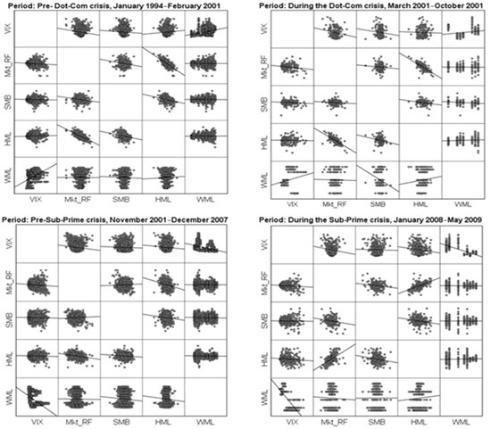
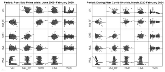
Figure 1.
Multiple scatter dot matrix, representing the correlations of the five endogenous variables across the periods of the study.
Observing both the table with the correlation coefficients and mainly the image with the scatter graphs, it follows that the correlation mechanisms of the variables change over time, both between the periods examined by the research, as well as within the periods. The change in the correlation mechanism within a selected period implies that there are probably structural events that change the behaviour of the market at time points other than the selected ones that mainly come from NBER. However, we ignore the structural breaks, and any relevant testing, for simplicity.
4.2. Stationarity Tests: Augmented Dickey–Fuller Tests
Table 5 represents the results of the augmented Dickey–Fuller stationarity tests. Firstly, we assume that the process of creating the variables (data generating process) remains unchanged throughout time. Therefore, for Augmented Dickey–Fuller (ADF) tests it is not necessary to split the sample into sub-periods. The ADF control of one variable yt has the following generalized form:
where t is the time, and Δ(∙) the differences of each variable. With the ADF test, the following hypothesis has been tested:
H0:
γ = 0
H1:
based on the critical values of the statistics. These statistics are also represented, via E Views, in the “Test critical values” field of Table 5.γ < 0
Table 5.
Unit Root Tests for the stationarity of the variables.
If H0 is valid, then the variable yt has a unit root and is not stationary. In our case, from the graphs made in E Views, the variables are very close to 0 (mean value). Therefore, we can assume a0 = 0. It is also noticed that there is no trend, so we can assume that a2 = 0. According to Enders (2015), an ARIMA(p,1,q) process can be approximated by an ARIMA(n,1,0) process for sufficiently large n, so (ADF1) is an appropriate form even if the yt process is an ARMA(p,q) for p,q ≥ 1. Finally, lmax is chosen according to the Schwartz criterion (Enders 2015). Therefore, this lmax provides the smallest “SIC” value. From all the above, the ADF test that is applied is presented below:
where yt represents each of our endogenous variables. The null H0: γ = 0 and its alternative remain as it was previously formulated. In Table 5 below, all five endogenous variables (MKT_RF, SMB, HML, WML, DVIX) are stationary and indeed with a p-value ≈ 0. So, for each of the variables, the null hypothesis is rejected (H0: γ = 0) (level of significance <1%), and we can conclude—with relative certainty—that the MKT_RF, SMB, HML, WML, and DVIX time series are stationary. Documenting that they are stationarity is necessary in order to estimate the VAR models in the next subsection.
4.3. Granger Causality Tests
In our analysis, pairwise Granger causality testing will be applied. In the first part of the pairwise Granger causality test for the variables Xt and Yt, the following VAR(p) model is estimated:
and then the following hypothesis is tested:
- -
- For variables Yt
- -
- For variables Xt
Table 6.
Granger Causality Tests (comparing pre- and post-crisis for the two economic crises).
Furthermore, Table 6 below contains the Granger causality for the period before the Sub-Prime crisis and during the Sub-Prime crisis. In the period before the Sub-Prime crisis, there is a complaint against Granger (the corresponding H_0 is rejected) (Ι) from the market premium to the size factor, to the premium of value stocks over growth, and to momentum; (II) from the premium of value stocks to the size factor; (III) from momentum to the size factor; and (IV) from investor fear to the size factor, to the premium of value stocks over growth. However, during the period of the Sub-Prime crisis, the Granger causality remains from the momentum and investors’ fear to the size factor, as before this crisis, and a two-way causality is created between the market premium and the factor of size.
These findings agree to some extent with those of Durand et al. (2011) for the entire period before, during, and after Dot-Com (before Sub-Prime). Thus, it is observed that the risk premium affects both the size and value factor, and investors fear the size factor, only before and after Dot-Com. It is therefore important to separate the analysis into sub-periods depending on whether there are financial disturbances or not. Also, we see that investor fear is starting to affect the value factor after the end of the Dot-Com crisis. At this point, we should mention the following contradiction: our results deviate from the results of Durand et al. (2011), who found anti-Granger causality from investor fear to all premiums. It is therefore obvious that if the sample is split into sub-periods, then this complaint disappears, while fear seems to affect only the factor of the size. But investors’ fear seems to be triggered by the factor of size and momentum, all the way back to Dot-Com.
On the other hand, Durand et al. (2011) found that all factors except momentum affect fear. Also, the market is affected by momentum, which is expected, at least in times of smoothness; as a stock’s momentum increases the market is adapted to this increase as well. Finally, the risk premium also affects the factor of size and value, as found by Durand et al. (2011) but only until the Dot-Com crisis. Then, as it is observed, only the value factor affects the risk premium, as we expected from the results of Durand et al. (2011). Briefly, this means that the explanatory power of our endogenous variables to predict or cause market movements (as excess returns over risk-free) is small. This is to be expected, because if we could predict the market, things would be very different. Finally, we notice that the Dot-Com crisis and the Sub-Prime crisis differ greatly. In the first, there was no correlation between the endogenous variables, while in the second we found several. This, perhaps, is due to the duration of the two crises. The Dot-Com and subsequent US recession lasted less than a year, while the post-Sub-Prime recession lasted almost two years. The stock market disruption lasted less, but in any case, within two years, investors adjusted their behaviour, and we can see this in the existence of objections during the Sub-Prime crisis.
It is important to note that after each crisis, there is a notable shift in the connections between the internal factors. This is evident especially during times of crisis, when existing relationships are disrupted, and new patterns emerge. However, an interesting exception to this trend can be observed after the Sub-Prime crisis. As we will see in the next section on VAR estimation, there are no clear causal effects or interactions among the variables. This could be due to the significant transformative impact of the 2007–2008 crisis, or the monetary policies implemented by major central banks, which have greatly influenced yields and market dynamics.
4.4. Vector Autoregression (VAR) Estimates, before and after Crises
After having proved that the endogenous variables are stationary, and examined Granger causality, we can move on to VAR analysis. The analysis we do at this point concerns the two crises for which we have comparative data before and after the crisis. The VAR models, in their general form, are presented as follows:
(VAR1) in its most compact form:
although in some estimations, a second-order lag was not needed, i.e., C2 = 0. The vector Z that represents the endogenous variables is also used by Durand et al. (2011): contains five dummy variables, JAN, MON, TUE, WED, THU, each of which takes the value 1 if we have, respectively, January, Monday, Tuesday, Wednesday, Thursday. The days of the week were chosen because differences are observed in the returns of the stocks and the considered premiums depending on the days of the week, while January was chosen because the SMB has been observed to be higher during this month (Durand et al. 2011). The number of lags was automatically selected in the E Views environment, based on the overall Akaike criterion (AIC) according to Lütkepohl (2005). That is, with the possibility of (VAR1) having up to 10 lags, for each sub-period, as many as minimized the AIC as by Lütkepohl (2005) and Enders (2015) were finally selected.
In Table 7 below, we have the estimates of (VAR1), with one lag based on AIC, for the period before the Dot-Com crisis. From the results we observe that the market premium (MKT_RF) is not affected by any of the other variables nor by any autoregressive process. However, as it can be seen, the market premium has a statistically significant (5%) and positive effect on the size premium, on the value-to-growth premium, and a negative but statistically significant (5%) effect on the momentum factor. That is, a positive development in the market has a positive significant effect on the difference in the returns of companies with lower capitalization versus those with smaller returns, and those with a large book-to-market value. On the contrary, it undermines the stocks which have had consistently large and positive returns in the past period. Therefore, before the Dot-Com crisis, a positive market development favoured small-cap stocks, stocks with a high book-to-market ratio, and stocks that were not as profitable in the past. At the same time, this effect seems to have disappeared from the market since the Dot-Com crisis and then with the only exception in the period before the Sub-Prime crisis when a rise in the market favoured the returns of stocks with a high book-to-market ratio (HML).
Table 7.
Vector Autoregression estimates.
These results are more in agreement with those of Durand et al. (2011), who examined only Granger causality and found that the risk premium causes (Granger) the size and value factor and fear. In addition, we are also impressed by the non-effect of fear on the pre-danger. Intuitively, we would expect an increase in investor fear to lead in liquidations and a shift to risk-free securities, reducing the market premium.
Remaining in the period before the Dot-Com crisis, we observe that the effect of the size premium was also significant. This has a positive and statistically significant (5%) effect on the premium of the returns on value shares and the fear of investors, while it has a negative effect on momentum, favouring the shares that recently had the lowest returns. Therefore, an increase in the premium of the returns of companies with lower capitalization favoured the returns of value stocks and increased the fear of investors, while it also favoured more those stocks that recorded lower returns recently. The effect of SMB with momentum, however, is bidirectional as the latter positively affects the return premium of smaller capitalization companies. Finally, this influence of SMB on these variables ceases to apply at the discretion of Dot-Com and thereafter.
Concluding the analysis of the VAR estimates for the period before the Dot-Com crisis (Table 7 below), we observe that investor fear does not appear to affect or be affected (except for SMB) by any of the three Fama, French, and Carhart factors. On the contrary, fear seems to be affected by the days of the week. As for the days of the week, it seems that on Mondays, investors turned to the stocks of companies with larger capitalization (flight to quality), increasing their returns and reducing SMB. In addition, momentum is negatively affected by almost all variables except DVIX which does not affect it at all. Finally, all the regressions for this period have a very low adjusted R2, meaning that despite the statistically significant effects, these seem to explain only a specific part of the variability of the endogenous variables.
However, we are also impressed by the non-effect of fear on any of the factors. We would expect that the increase in fear would direct investors to safer stocks (value) and to safer companies (high capitalization), increasing the returns of these, therefore, increasing their premium. However, this does not happen either during the normal period before the Dot-Com crisis nor during the Dot-Com crisis.
For the period during the crisis, in Table 7, we have the 1-lag VAR estimates based on the AIC criterion. From this period, there are no statistically significant estimates except for the day-of-the-week dummy variables. Monday has a negative effect on the returns of smaller-cap stocks and a positive effect on investor fear—investors fear Mondays more! We notice that even in the Dot-Com crisis none of the premium is affected by fear, and this contradicts the findings of Durand et al. (2011), who found Granger causality to all endogenous variables. The differences in estimates are greater since the sample was split into sub-periods of economic recovery and recession, while Durand et al. (2011) examined the entire time period.
Table 7 also represents the VAR estimates, with two lags based on the AIC criterion for the period before the Sub-Prime crisis. During this period, a rise in the market appears to favour value stock returns, while conversely, the effect is opposite to an increase in value stock returns, negatively affecting the market premium. The increase in value stock returns positively affects the return premium of small-cap stocks and stocks that previously had lower returns. The size factor affects HML and investors’ fear: in terms of exogenous variables, investors seem to be more afraid of Mondays, and this day (along with Thursday) favours the returns of growth stocks.
Finally, the estimated VAR model manages to explain to a small extent the variability of the endogenous variables. In fact, the only element that impresses us is the non-effect of fear on the remaining endogenous variables. It appears, therefore, that fear does not cause changes in the individual endogenous variables, in any premium despite the contrary findings of Durand et al. (2011) that fear has a statistically significant effect. It seems, therefore, that the different specialization of the model because of the sub-periods led to different results from those of Durand et al. (2011). On top of that, in Table 7 we have the estimates of (VAR1), with two lags based on AIC, for the period during the Sub-Prime crisis. During the Sub-Prime crisis, we see a two-way and positive influence between the market premium and the premium of lower capitalization firms. That is, positive developments in the market favoured the returns of stocks with the lowest capitalization and vice versa. In general, during this crisis as well, it seems that there are no effects between the endogenous variables. And, in this period, the estimated VAR model manages to explain to a small extent the variability of the endogenous variables (R2 < 11%).
For the post-Sub-Prime crisis period, in Table 7, we have the 1-lag VAR estimates based on the AIC criterion. During this period, we observe that increasing value stock returns had a positive effect on the returns of the lowest capitalization stocks, while we do not estimate any other effect among the endogenous ones. Moreover, during this period, investor fear increases on Mondays. Finally, the estimated VAR model manages to explain only to a small extent the variability of the endogenous variables (R2 < 3%).
To summarize, from the VAR estimates concerning the five sub-periods we can state the following: (a) investor fear on the first day of the week (Monday) is systematically higher on average in all sub-periods except during the Sub-Prime crisis; (b) since the Dot-Com crisis the interaction effects between endogenous variables are permanently broken and corresponding relationships do not seem to appear again to such an extent; (c) fear does not cause changes nor other effects on premiums or on momentum factor; and (d) after the Sub-Prime crisis, the explanatory power of our VAR model based on the adjusted coefficient of determination (R2) is practically annihilated. Briefly, fear does not seem to affect premiums, neither does momentum, but the various results and conclusions of the existing literature are sensitive concerning the specificity of the models. Thus, Durand et al. (2011) find statistically significant effects of fear, and splitting the time horizon into recession and boom sub-periods changes the specification of the model and, thus, changes the results. Moreover, loose monetary policy may be what is now fuelling changes in bond values, and this is reflected in the annihilation of the interpretive power of VAR estimates. In the next subsection, it is examined how these statistically significant effects of the above VAR models are formed.
4.5. Results from Impulse Responses
The analysis of Durand et al. (2011) focuses on the effect of fear (VIX) on the remaining endogenous variables, an effect that we could not document either with the VAR models or with the Granger causality analysis. For the endogenous variables based on VARs, it is mentioned that there is a statistically significant effect on other endogenous variables. Thus, we consider it appropriate to examine each effect with an impulse response.
Assuming that the model (VAR1) is a system of endogenous variables, impulse response analysis shows the change in one endogenous variable from one standard deviation shock to one of another endogenous variable (Lütkepohl 2005). The shock means the error , i = 1, 2, …, 5 from the estimate of (VAR1). So, if we want to see the effect of MKT_RF on SMB with impulse response, then we see how SMBt reacts if we apply (VAR1) an error > 0. In Figure 2 below, we see on the vertical axis how each endogenous variable changes depending on the shock that is introduced each time to the system, while we see on the horizontal axis the moments the time when these changes take place. Since we have daily data, then on the horizontal axis we see days. Both the shocks and how they affect endogenous variables were selected based on the statistically significant effects we found in the previous subsection on VAR estimations.
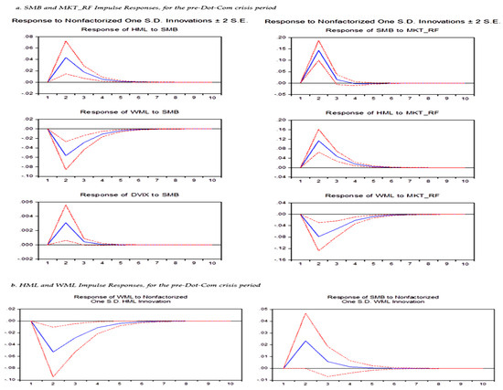
Figure 2.
SMB and MKT_RF Impulse Responses, for the pre-Dot-Com crisis period.
In Figure 2 below, for the Pre-Dot-Com crisis period, we observe the reaction of HML, WML, and DVIX after an SMB disruption. What we observe is that a positive disturbance in the premium of low capitalization stocks compared to low ones, has a positive effect for about 5–6 days on the premium of value stocks, negatively for 6–7 days on momentum, while the effect on fear is positive but short-term, lasting approximately 2–3 sessions.
For the pre-Dot-Com period, we notice that a positive disturbance in the market premium has a positive effect in the short term (3 sessions) on the size premium, but with a longer duration (6–7 days), on the premium of value shares. Moreover, a positive disturbance in the market premium has a negative effect for 6–7 days on the momentum factor. With a relatively long duration, an HML disturbance also affects the momentum factor. The magnitude factor reacts for a small period of time to a momentum shock. In general, in Figure 2 we observe that the effects received by the momentum, during this period, from the rest of the endogenous variables (except DVIX) are negative and persist for several days after the disturbance.
During the period of the Dot-Com crisis there was not any statistically significant effect between the endogenous variables and, therefore, we do not have an impulse response analysis for this period.
Figure 3 demonstrates how positive market trends contribute to the value stock premium in the pre-Sub-Prime crisis. This effect remains positive but temporary, lasting for a maximum of four days. During this period, disruptions impacting the premium of value stocks have short-time effects on the market premium and the size factor. However, for the momentum factor, the disturbance has a significant impact three days after the event. Notably, momentum initially has a positive effect on lower capitalization premium, followed by a subsequent negative impact.
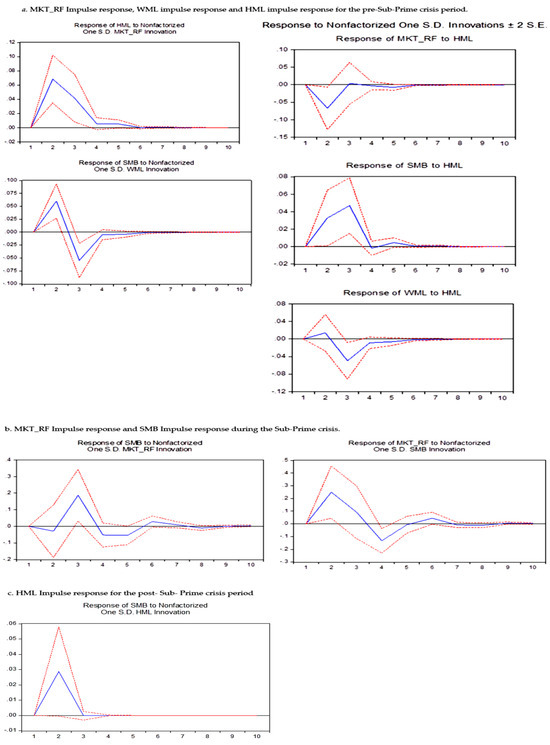
Figure 3.
Impulse Responses Results for the pre-Sub-Prime crisis period, during the Sub-Prime period, and the post-Sub-Prime period.
During the Sub-Prime crisis, there is only a two-way relationship between the size factor and the market premium, as seen in Table 7 above. However, the impulse response analysis shows that this effect has no statistically significant effects on the changes of these endogenous variables (Figure 3). Of course, the effect of SMB causes changes in long-term returns, sometimes positive and sometimes negative. But, only the changes on the second (positive market return change) and the fourth (negative) day are statistically significant.
Notably, prior to and during the Sub-Prime crisis, an interesting discrepancy is observed between the outcomes of the impulse response analysis and the VAR(2) model results shown in Table 7. This divergence is attributed to the emergence of effects in the VARs that are only apparent for one of the two lags, making it difficult to draw definitive conclusions from the impulse response analysis. However, the impulse response analysis and the Granger causality test ultimately concur, leading to a general inference. It is evident that from the Dot-Com crisis onwards, and especially after the Sub-Prime crisis, there is a visible trend of diminishing interactions among our endogenous variables.
5. Conclusions
The present research aimed to analyse the interactions between “investors’ fear”, the factors of the Fama and French model, the Carhart momentum factor, and the risk premium. Specifically, the effects between the variables, the direction of these effects (positive or negative), the existence of causal relationships (Granger causality), and the duration of the interactions after exogenous disturbances were examined. At the same time, it examined how the two financial crises, the Dot-Com and the Sub-Prime, affected these interactions. Further expanding the research of Durand et al. (2011), the present study focuses more extensively on these effects, considering the consequences of the two crises. Firstly, investor fear was observed to show an overall negative trend across periods, indicating a tendency for investors to feel more calm or safe on average after bursts of fear. Furthermore, it was observed that none of the risk premiums remain consistently positive, contrary to the assumptions of many previous studies. Subsequently, it was found that after each crisis, the relationships between the endogenous variables undergo significant changes, while many of them completely disappear. During crises, existing connections are broken and replaced by new ones after the crisis is over. Here, the VAR estimates for five different sub-periods showed the following: first, investor fear is systematically higher on average on Mondays than on other days, except during the Sub-Prime crisis period and the Dot-Com period crisis as well. Secondly, after the Dot-Com crisis, the interactions between the endogenous variables are permanently broken, while overall causality does not reappear at this level. The results of the impulse responses showed that the disturbances in the endogenous variables mainly last more than four days, with none of them representing a significant short-term duration. At the same time, it was observed that during periods of crisis, causality relationships are completely interrupted, while they are not restored with the recovery of the economy. In conclusion, it is noted that future research should focus on examining the effect of monetary policy on the relationships of valuation variables (i.e., Stock and Watson 2003). Furthermore, the recession period of 2007–2009 is of particular interest for understanding the evolution of investor behaviour within this time frame.
Regarding the COVID-19 crisis and concerning the correlation coefficients between the endogenous variables, the same behaviour was observed within this crisis as in the previous crises.
Also, in future research a few technical issues could be considered, including the use of the sup MZ test of Ahmed et al. (2017). This test allows algorithmic detection of any changes in volatility, caters to unknown breakpoints, and also compares it to the sup F. This test is useful in curing a key weakness of most regressions, the assumption that the correlation or regression coefficients remain constant in time, or that the structure of the model remains constant. It is a fact that the sup MZ test is a useful test. However, in the case of our research its usefulness is less than its average usefulness for two reasons: First, because it is appropriate to use break points from BERS, so that we are talking about commonly accepted recession periods; second and more importantly, in this paper we do not assume a uniform structure over the whole period, but we compute the coefficients at each period separately. In this way, our paper already contains the possibility to identify changes in the structure of the interaction between different time periods, which is one of the main research questions of our paper. However, the visual examination of the multiple scatter dot matrix shows the existence of a varying nature of the causing mechanism, between and possibly within the selected periods.
We acknowledge that our research has certain limitations, which could be addressed in future works. First, given that the Normal distribution is violated, using a more appropriate distribution, such as the Student’s t distribution, could offer a different modelling approach and potentially lead to different empirical results. Second, our empirical results might be sensitive to the presence of deterministic trends in the model’s volatility, which we assumed were absent in our analysis (see Andreou and Spanos (2003); Lu and Podivinsky (2003) for details). Third, as discussed in Kim and Ji (2015) and Michaelides (2021), the usage of varying levels of statistical significance might have been more appropriate due to the different sample sizes of our subsamples. Fourth, the model does not include the common CMA and RMW factors from Fama and French (2015) or the traded liquidity factor from Pástor and Stambaugh (2003).
To fully enrich the research and extend it in various contexts, it is crucial to conduct, in the future, a comparative analysis that should not just cover periods before, during, and after a crisis. Nevertheless, it should also consider different types of crises such as the post-pandemic crisis (since the during pandemic crisis period is already partially examined), the oil crisis, or crises in Ukraine and Gaza. By adopting this comprehensive approach, we can gain a deeper insight into the complexities of different crisis situations and enhance the strength and relevance of our research findings. By comparing the results with those from a pandemic-focused investigation, researchers can identify commonalities, distinctions, and key factors that impact the variables and causality relationships. Ultimately, this comparative framework will greatly broaden the implications of the research across a range of crisis situations.
Author Contributions
Conceptualization, A.P. and P.B.; methodology, P.B.; validation, P.B., K.T. and I.K.; formal analysis, A.P.; investigation, A.P.; data curation, A.P.; writing—original draft preparation, A.P., P.B. and K.T.; writing—review and editing, A.P., P.B., K.T. and I.K.; visualization, P.B. and K.T.; supervision, P.B.; project administration, P.B., K.T. and I.K. All authors have read and agreed to the published version of the manuscript.
Funding
This research received no external funding.
Data Availability Statement
No new data were created or analyzed in this study.
Conflicts of Interest
The authors declare no conflicts of interest.
References
- Agarwal, Vineet, and Richard Taffler. 2008. Does Financial Distress Risk Drive the Momentum Anomaly? Financial Management 37: 461–84. [Google Scholar] [CrossRef]
- Ahmed, Mumtaz, Gulfam Haider, and Asad Zaman. 2017. Detecting structural change with heteroskedasticity. Communications in Statistics—Theory and Methods 46: 10446–55. [Google Scholar] [CrossRef]
- Andreou, Elena, and Aris Spanos. 2003. Statistical adequacy and the testing of trend versus difference stationarity. Econometric Reviews 22: 217–37. [Google Scholar] [CrossRef]
- Barberis, Nicholas, Andrei Shleifer, and Robert Vishny. 1998. Model of Investor Sentiment. Journal of Financial Economics 49: 307–43. [Google Scholar] [CrossRef]
- Basdekis, Charalambos, Apostolos Christopoulos, Evgenios Gakias, and Ioannis Katsampoxakis. 2023a. The effect of ECB unconventional monetary policy on firm’sperformance during the global financial crisis. Journal of Risk and Financial Management 16: 258. [Google Scholar] [CrossRef]
- Basdekis, Charalambos, Ioannis Katsampoxakis, and Konstantinos Anathreptakis. 2023b. Women’s Participation in Firms’ Management and Their Impact on Financial Performance: Pre-COVID-19 and COVID-19 Period Evidence. Sustainability 15: 8686. [Google Scholar] [CrossRef]
- Campello, Murillo, Long Chen, and Lu Zhang. 2008. Expected Returns, Yield Spreads, and Asset Pricing Tests. Review of Financial Studies 21: 1297–338. [Google Scholar] [CrossRef]
- Carhart, Mark M. 1997. On Persistence in Mutual Fund Performance. The Journal of Finance 52: 57–82. [Google Scholar] [CrossRef]
- Chaudhary, Rashmi, Priti Bakhshi, and Hemendra Gupta. 2020. Volatility in international stock markets: An empirical study during COVID-19. Journal of Risk and Financial Management 13: 208. [Google Scholar] [CrossRef]
- Durand, Robert B., Alex Juricev, and Gary W. Smith. 2007. SMB–Arousal, Disproportionate Reactions and the Size-Premium. Pacific-Basin Finance Journal 15: 315–28. [Google Scholar] [CrossRef]
- Durand, Robert B., Dominic Lim, and J. Kenton Zumwalt. 2011. Fear and the Fama-French Factors. Financial Management 40: 409–26. [Google Scholar] [CrossRef]
- Enders, Walter. 2015. Applied Econometric Time Series, 4th ed. Hoboken: John Wiley & Sons. [Google Scholar]
- Fama, Eugene F., and Kenneth R. French. 1993. Common Risk Factors in the Returns on Stocks and Bonds. Journal of Financial Economics 33: 3–57. [Google Scholar] [CrossRef]
- Fama, Eugene F., and Kenneth R. French. 2015. A five-factor asset pricing model. Journal of Financial Economics 116: 1–22. [Google Scholar] [CrossRef]
- Grinblatt, Mark, and Bing Han. 2005. Prospect Theory, Mental Accounting, and Momentum. Journal of Financial Economics 78: 311–39. [Google Scholar] [CrossRef]
- Guo, Zhaojun, Yajun Shen, Zheyi Tang, and Luyuan Wang. 2022. The Research of Fama-French Three-factor Model’s Applications in the Chinese Stock Market after the Financial Crisis. Paper presented at the 2022 7th International Conference on Financial Innovation and Economic Development (ICFIED 2022), Zhuhai, China, January 14–16; Berlin and Heidelberg: Atlantis Press, pp. 799–805. [Google Scholar] [CrossRef]
- Horvath, Dominik, and Yung-Lin Wang. 2021. The examination of fama-french model during the COVID-19. Finance Research Letters 41: 101848. [Google Scholar] [CrossRef] [PubMed]
- Houge, Todd, and Tim Lughran. 2006. Do Investors Capture the Value Premium? Financial Management 35: 5–19. [Google Scholar] [CrossRef]
- Jegadeesh, Narasimhan, and Sheridan Titman. 1993. Returns to Buying Winners and Selling Losers: Implications for Stock Market Efficiency. Journal of Finance 48: 65–92. [Google Scholar] [CrossRef]
- Kim, Jae H., and Philip Inyeob Ji. 2015. Significance testing in empirical finance: A critical review and assessment. Journal of Empirical Finance 34: 1–14. [Google Scholar] [CrossRef]
- Konstantinov, Gueorgui S., and Frank J. Fabozzi. 2021. Towards a dead end? EMU bond market exposure and manager performance. Journal of International Money and Finance 116: 102433. [Google Scholar] [CrossRef]
- Kostin, Konstantin B., Philippe Runge, and Leyla E. Mamedova. 2022. Validity of the Fama-French Three-and Five-Factor Models in Crisis Settings at the Example of Select Energy-Sector Companies during the COVID-19 Pandemic. Mathematics 11: 49. [Google Scholar] [CrossRef]
- Kumar, Alok, and Charles MC Lee. 2003. Individual Investor Sentiment and Comovement in Small Stock Returns. Cornell University Department of Economics Working Paper. Available online: http://ssrn.com/abstract=328980 (accessed on 17 December 2023).
- La Porta, Rafael, Josef Lakonishok, Andrei Shleifer, and Robert Vishny. 1997. Good News for Value Stocks: Further Evidence of Market Efficiency. Journal of Finance 52: 859–74. [Google Scholar] [CrossRef]
- Lu, Maozu, and Jan M. Podivinsky. 2003. The Robustness of Trend Stationarity: An Illustration with the Extended Nelson–Plosser Dataset. Econometric Reviews 22: 261–67. [Google Scholar] [CrossRef]
- Luehlfing, Michael S., William R. McCumber, and Huan Qiu. 2023. CEO Social Capital and the Value Relevance of Accounting Metrics. Risks 11: 78. [Google Scholar] [CrossRef]
- Lütkepohl, Helmut. 2005. New Introduction to Multiple Time Series Analysis. Berlin and Heidelberg: Springer. [Google Scholar]
- MacKinnon, J. G. 1996. Numerical distribution functions for unit root and cointegration tests. Journal of Applied Econometrics 11: 601–18. [Google Scholar] [CrossRef]
- Merton, Robert C. 1980. On Estimating the Expected Return on the Market: An Exploratory Investigation. Journal of Financial Economics 8: 323–61. [Google Scholar] [CrossRef]
- Michaelides, Michael. 2021. Large sample size bias in empirical finance. Finance Research Letters 41: 101835. [Google Scholar] [CrossRef]
- Mlawu, Lonwabo, Frank Ranganai Matenda, and Mabutho Sibanda. 2023. Linking Financial Performance with CEO Statements: Testing Impression Management Theory. Risks 11: 55. [Google Scholar] [CrossRef]
- Pástor, Ľuboš, and Robert F. Stambaugh. 2003. Liquidity risk and expected stock returns. Journal of Political Economy 111: 642–85. [Google Scholar] [CrossRef]
- Petkova, Ralitsa, and Lu Zhang. 2005. Is Value Riskier than Growth? Journal of Financial Economics 78: 187–202. [Google Scholar] [CrossRef]
- Roll, Richard. 1981. A Possible Explanation of the Small Firm Effect. Journal of Finance 36: 879–88. [Google Scholar] [CrossRef]
- Rozeff, Michael S., and Mir A. Zaman. 1998. Overreaction and insider trading: Evidence from growth and value portfolios. The Journal of Finance 53: 701–16. [Google Scholar] [CrossRef]
- Shumway, Tyler. 1997. The delisting bias in CRSP data. The Journal of Finance 52: 327–40. [Google Scholar] [CrossRef]
- Stock, James H., and Mark W. Watson. 2003. Forecasting output and inflation: The role of asset prices. Journal of Economic Literature 41: 788–829. [Google Scholar] [CrossRef]
- Vassalou, Maria, and Yuhang Xing. 2004. Default Risk in Equity Returns. Journal of Finance 59: 831–68. [Google Scholar] [CrossRef]
- Viippola, Valtteri. 2020. Corporate Social Responsibility’s Effect on Stock Returns during the COVID-19 Crisis: Evidence from US Markets. Bachelor’s thesis, Aalto University, Espoo, Finland. [Google Scholar]
Disclaimer/Publisher’s Note: The statements, opinions and data contained in all publications are solely those of the individual author(s) and contributor(s) and not of MDPI and/or the editor(s). MDPI and/or the editor(s) disclaim responsibility for any injury to people or property resulting from any ideas, methods, instructions or products referred to in the content. |
© 2024 by the authors. Licensee MDPI, Basel, Switzerland. This article is an open access article distributed under the terms and conditions of the Creative Commons Attribution (CC BY) license (https://creativecommons.org/licenses/by/4.0/).