Resource Price Interconnections and the Impact of Geopolitical Shocks Using Granger Causality: A Case Study of Ukraine–Russia Unrest

Abstract

Political events significantly impact economic indices, including agricultural commodities. While Granger causality is a well-established method for analyzing interdependencies between time series data, its traditional application can be challenging to interpret across multiple periods. This research enhances the Granger causality method to quantify changes in the interlinkages among variables over time, offering a more intuitive framework for analyzing how political events affect economic indices. The proposed method involves conducting Granger causality tests across different periods, forming vectors from the results to capture transitions from Granger-causing to non-Granger-causing variables. These vector amplitudes provide quantitative measures of changes with explanatory power over time. The dataset includes eight variables over a decade, focusing on the following major geopolitical events: the Russian occupation of Crimea in 2014 and the invasion of Ukraine in 2022, with an intermediate “no-shocks” period as the reference. The results show significant changes in the interlinkages among the variables during crisis periods compared to stable periods. This enhanced method provides valuable insights, informing trading strategies and risk management during periods of geopolitical instability. This innovative approach offers a novel tool for market participants to better understand and respond to economic shocks caused by political events.

1. Introduction

In the final quarter of 2021, Russian armed forces initiated extensive military exercises near Ukraine’s borders, sparking international concerns of a potential full-scale invasion, despite continuous denials by the Russian government. However, on 24 February 2022, Russian military forces invaded Ukraine, marking the first large-scale military operation on European soil since World War II. Both Ukraine and Russia are significant producers of wheat and other crops, leading to heightened interest in commodity availability in the physical market before and after the conflict. Consequently, global commodity markets have experienced increased volatility and record-high wheat prices. The two nations previously clashed in a similar conflict in 2014, when Russia occupied Crimea with minimal military action. In our study, we focus on these two unrest periods separated by eight years with no significant events between the countries.

The conflicts have had a profound impact on agricultural commodity prices, particularly those closely tied to the involved nations. Agricultural commodity prices play a crucial role in the global economy, serving as trading assets, hedging products, and references for long-term contracts. They also significantly influence the income of farmers worldwide. Extensive research has explored the effects of government interventions, such as subsidies, on critical commodity prices. Wheat, historically fundamental for Europe, North America, Africa, and the Middle East, holds immense importance as one of the world’s primary agricultural commodities (Miljkovic 2004; Mohtadi and Castells-Quintana 2021).

Researchers have addressed the need to interpret the behavior of agricultural commodity prices and, at the same time, have introduced phenomena that have qualitative behaviors, such as climate conditions or severe weather impacting the yield, availability, or produced quantities in critical production areas. The price of commodities has been an important historical issue and, thus, has been recorded and examined for over seven centuries (Awaworyi-Churchill et al. 2022). There has been extensive research on the relationships between agricultural commodities’ prices, other commodities, and exchange rates (Nazlioglu and Soytas 2012). Additionally, political analyses have been recorded, as major foundations are monitoring the subject (Haniotis and Baffes 2010). Recently, political decisions, previously in the form of subsidies or tariffs, have affected the prices of agricultural commodities. These decisions include sanctions on the export of several goods produced in various countries as a form of economic pressure to balance political initiatives. This form of trade war counters the principles of globalization, and to add more severity to this situation, actual acts of war have occurred occasionally. The military clash between the Russian Federation and Ukraine at the beginning of 2022 has already attracted attention from researchers, who have examined the potential outcomes of the conflict for a variety of economic indices (Costola and Lorusso 2022; Lo et al. 2022; Manelli et al. 2024; Sokhanvar and Bouri 2023).

Russia and Ukraine, respectively, have ranked third and seventh globally (

Table 1. Average global production of wheat between 2013 and 2022 for top ten countries.

Area	Production
China, mainland	132.2
India	99.5
Russian Federation	74.6
United States of America	52.3
France	36.6
Canada	31.4
Ukraine	25.6
Pakistan	25.6
Australia	24.7
Germany	23.8

Note: FAOSTA data accessed May 2024, in millions of tons.

) in wheat production (FAOSTAT data accessed on May 2024), and are key contributors to the global wheat supply. The conflict between these major wheat producers has sparked concerns about wheat availability in global markets.

Both countries (and especially Ukraine) contribute significantly to the global trade of wheat, as they export a sizable portion of their production, as demonstrated in

Table 2. Russian and Ukrainian production and export of wheat between 2013 and 2022.

	Year	2013	2014	2015	2016	2017	2018	2019	2020	2021	2022
Russian Federation	Production	52.1	59.7	61.8	73.3	86.0	72.1	74.5	85.9	76.1	104.2
	Export Quantity	13.8	22.1	21.2	25.3	33.0	44.0	31.9	37.3	27.4	17.8
	Export %	26%	37%	34%	35%	38%	61%	43%	43%	36%	17%
Ukraine	Production	22.3	2 4.1	26.5	26.1	26.2	24.7	28.4	24.9	32.2	20.7
	Export Quantity	7.8	10.5	13.5	17.9	17.3	16.4	20.0	18.1	19.4	11.2
	Export %	35%	44%	51%	69%	66%	66%	71%	72%	60%	54%

Note: FAOSTA data accessed May 2024, in millions of tons.

. Consequently, wheat prices in the global markets have been significantly affected. The impact on US wheat prices has been documented as being more severe than elsewhere (Patel 2024). This impact, in turn, has affected commodity stock prices and, therefore, the wheat prices being determined in the global stock markets. The concerns around the regional events have also been documented and analyzed by the Food and Agriculture Organization and The State of the World series issue for Agricultural Commodity Markets (FAO Knowledge Base 2022).

As illustrated in Table 2, Ukraine’s exports share of the overall production is higher than that of Russia. Additionally, the exported volume of wheat from Ukraine had a significant increase between 2013 (7.8M tons) and 2021 (19.4M tons), slowing down in 2022, probably due to the offence by Russia. An increase, with a declining trend for the year 2022, in Russian exports is also evident.

Moreover, the prolonged military activities in the Black Sea, a vital region for transporting crops from Russia, Ukraine, and neighboring countries, pose a significant risk to commodity availability. Discussions have highlighted the substantial connection between commodity prices and the dry bulk shipping segment, particularly in the Black Sea region (Melas and Michail 2021).

Commodity prices are known to fluctuate, as indicated in the literature (Barros et al. 2022; Makkonen et al. 2021; Salisu et al. 2019), while factors like the global economy, climate conditions, inflation, and GDP are the sources of this fluctuation. A comprehensive literature review suggests that a time series approach is well suited for analyzing commodity price behavior, with specialized software often utilized for this purpose. EViews (version 12) software, in its various editions, has been frequently employed for such analyses, as documented in (Hua 1998; Makin 2013; Xiong et al. 2015).

In this study, we focus on wheat prices as the primary indicator linked to geopolitical events during the period of interest. Wheat holds significant cultural importance for Ukraine, often referred to as the “wheat farm of Europe and the former USSR”. This cultural significance is evident in Ukraine’s national flag, which was inspired by the image of yellow wheat fields beneath a blue sky. Through our research, we aim to demonstrate the interlinkages between wheat prices and geopolitical events using our proposed methodology.

Maize (corn) is the second agricultural commodity included in our analysis. Russia and Ukraine are significant producers of maize, ranking 11th and 5th, respectively, in global production quantities for 2021 (Food and Agriculture Organization of the United Nations FAOSTAT 2022). Additionally, we employ other financial indicators with relations to agricultural commodities that have been established and validated by the existing literature. As noted in (Xiong et al. 2015), commodities have predictive power for stock returns, leading us to include two stock market indices—the DAX for the European Union and the S&P 500 for the United States—due to their diverse composition of stocks and the relevant literature overview (Brooks and Prokopczuk 2013). Given the turmoil of the period under examination, we incorporate gold and crude oil (as reflected in the Brent index) as hedging options during periods of economic uncertainty (Junttila et al. 2018; Mensi et al. 2022). Furthermore, we include daily exchange rates for EUR/USD, as the most traded global exchange rate, and for EUR/RUB as a Russia-specific indicator.

With the relevance of these indicators established, our research addresses the following questions: Can the complex results of multiple Granger causality tests be transformed into a comprehensive output? Is there a method by which to measure the transition of independent variables from explanatory to non-explanatory and vice versa? These questions are pivotal for understanding the dynamics of our analyzed variables, particularly during politically triggered shocks. Whereas performing multiple Granger causality tests is not extremely challenging, simultaneously interpreting the results and identifying shifts in the explanatory variables across numerous periods can be complex.

In a recent, state-of-the-art review paper (Shojaie and Fox 2022), the various expansions and applications of Granger causality are presented along with their advantages and possible drawbacks. However, despite the importance of these extensions of the theory, and the presented inherent restrictions of the methodology, there is no reference to the behavior of causal shifts among different time periods, thus allowing us to address this as a research gap to be filled with a novel methodology. For the discrimination of time periods, a shock (political in our research) is utilized along with a distinctive breakpoint, identified by a proper analysis as described hereinafter.

The presented GVIM methodology provides a fast and quantitative representation of the outputs, simplifying this task. The simplicity of this method is novel, according to the existing literature, and can be easily applied by market participants who lack an extensive mathematical background. It provides a diagnostic tool comprising sets of numbers that indicate shifts in the explanatory variables, making it accessible and useful for those who may find the outputs of multiple Granger causality tests challenging to interpret.

2. Data and Methodology

The data utilized for analyzing the behavior of all indices were sourced from the online databank investing.com (accessed on 20 September 2022), and processed using EViews version 12. The initial data formulation involved dated values, with a total of 3530 daily entries in each time series. The commodities’ prices are US futures prices, traded on the Chicago commodities exchange and the NYSE. The US futures price for wheat is considered to be the predominant price indicator (Patel 2024) for global trade. The connectedness between agricultural commodities futures and stock values has been extensively researched and proven by (Cagli et al. 2023; Gorton and Rouwenhorst 2006), and is mainly attributed to hedging and speculative transactions on commodities by the same market players that simultaneously participate in stock exchange trading (Patel 2024). Considering a five-day workweek, missing values due to holidays or other exceptional days were treated as steady, adopting the last available date value.

The applied methodology encompassed several steps: transforming all the time series into a stationary form, a prerequisite for further analysis; conducting a breakpoint analysis to identify price shocks during specific periods; Vector Auto Regression modeling of the time series; and performing Granger causality tests tailored to each period.

Finally, the novel Granger Vector Interpretation Method (GVIM) was employed to interpret the results of the Granger causality tests, providing a unique approach for understanding the causal relationships among variables.

2.1. Stationarity

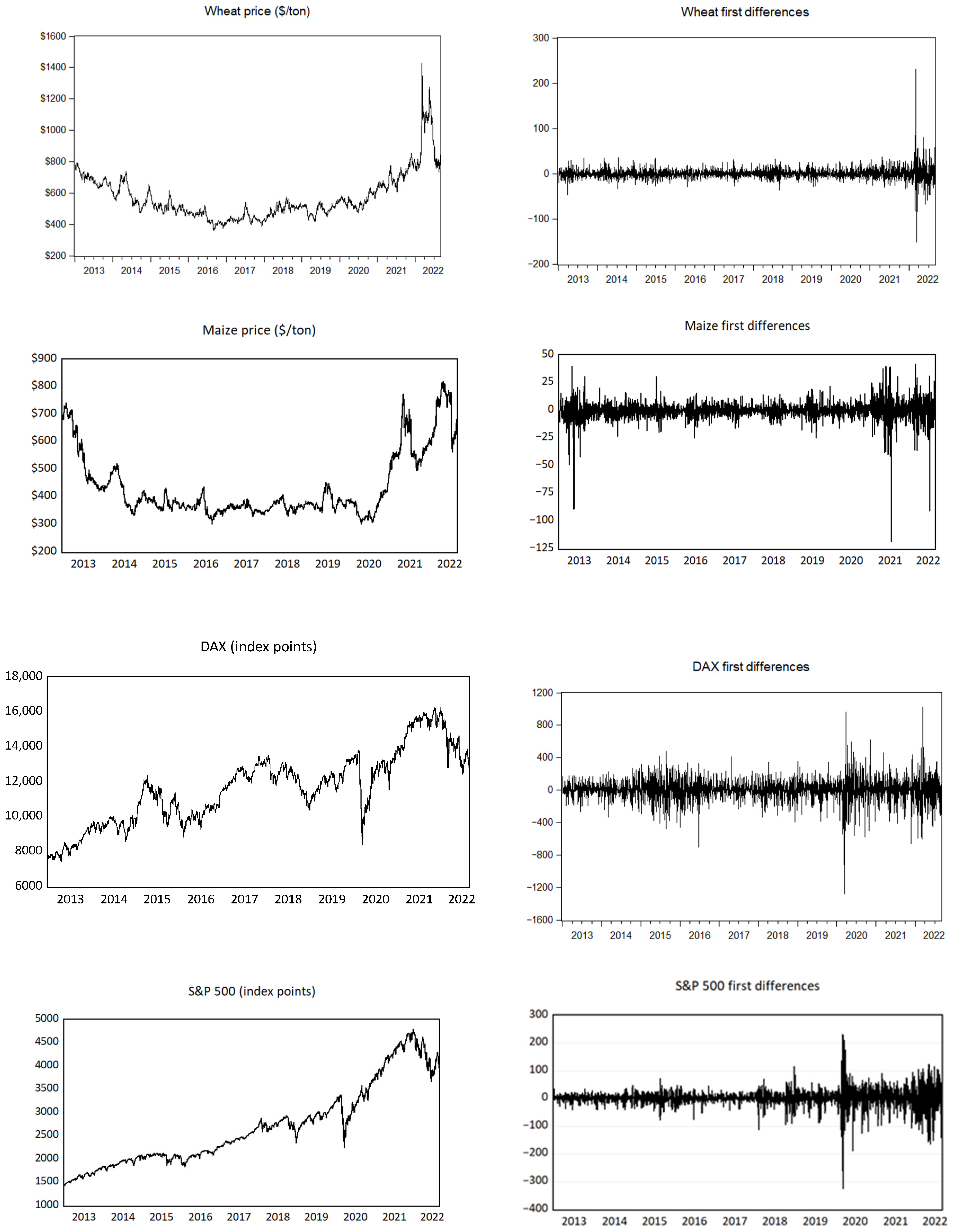
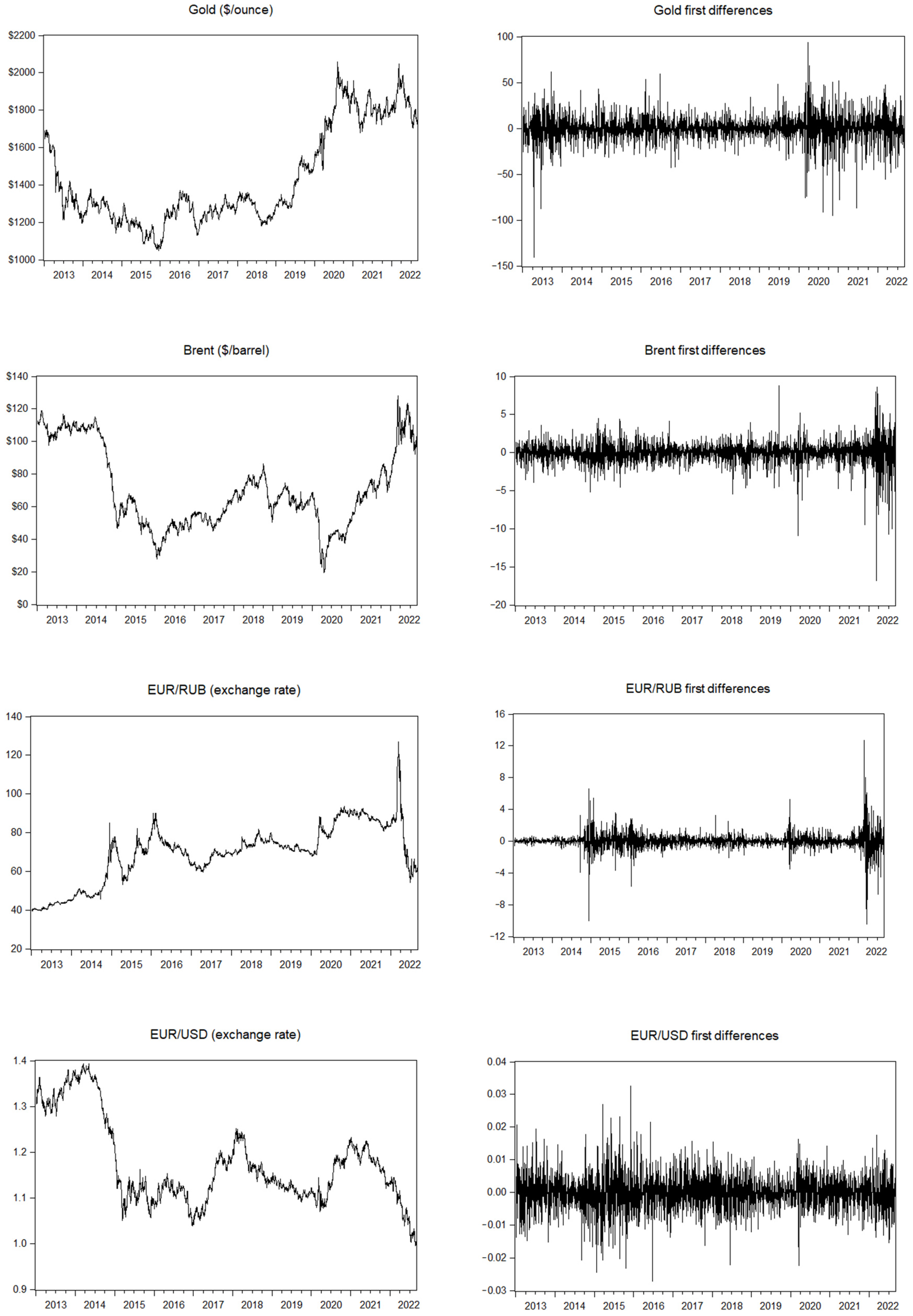
From our observations of the variable graphs, it was evident that none of the series exhibited stationarity. This was further confirmed by the software’s built-in Augmented Dickey–Fuller test with Schwarz information criterion, indicating a significant presence of intercept and/or trend. The stationarity test results are presented in

Table 3. Stationarity test for the time series with first differences.

Variable	Mean	Max.	Min.	Std. Dev.	Skew	Kurt	J-B	ADF	Sch. Crit.
Wheat	0.015	231.000	−152.000	11.220	1.609	75.183	767,882	−25,845	7653
Maize	−0.008	42.250	−118.750	7.011	−2.818	48.223	305,473	−58,025	6737
DAX	1.479	1016.420	−1277.550	118.035	−0.580	14.474	19,561	−61,684	12,383
S&P500	0.716	230.380	−324.890	26.690	−1.128	22.924	59,135	−15,344	9387
Gold	0.013	93.800	−140.300	12.219	−0.846	16.756	28,254	−62,075	7846
Brent	−0.004	8.800	−16.840	1.272	−1.271	22.168	54,993	−60,718	3322
EUR/RUB	0.006	12.740	−10.435	0.869	0.088	42.317	227,372	−57,927	2562
EUR/USD	−0.000	0.033	−0.027	0.005	0.009	6.882	2216	−60,528	−7868

Max—maximum; Min—minimum; Std. dev—standard deviation; Skew—skewness; Kurt—kurtosis; J-B—Jarque–Berra; ADF—Augmented Dicky–Fuller test; Sch crit.—Schwartz criterion.

, along with the corresponding parameters for all the time series.

To attain stationarity, first differences were incorporated following the standard theoretical equation, as suggested in (Mensi et al. 2022; Dimelis 2003) and consistent with our previous studies (Koutroumanidis et al. 2009).

$$y_t-y_{t-1}=a_0+u_t$$

(1)

where y_t and y_t−1 are the current and previous values of the variable,

a₀ is a constant, and

u_t represents the residual term, which is assumed to be white noise with zero mean and constant variance.

In Appendix A, the graphs for the examined variables are shown in their original form and after achieving stationarity with the application of first differences, as per Equation (1).

2.2. Breakpoint Analysis

Following the transformation of the series into a stationary form, the presence of an event causing a sudden change in a variable’s price is examined using the breakpoint analysis method. By aligning the breakpoint analysis outcome dates with observed political events, a temporal correlation between the variable price change and political events (such as the Russo-Ukrainian regional conflict) can be extracted. As described in (Remy Habimana 2016; Jones and Molitoris 1984) any non-stationary time series can be divided into intervals satisfying the stationarity criteria of stable mean and variance, with the change from one period to another considered a breakpoint. In the case of transformed time series using the first differences method, as discussed above, the breakpoint is defined as a point in time when the variance significantly changes, indicating a notable shift in the variable’s price recorded from global market information and trade.

The original paper by Vogelsang and Perron (Vogelsang and Perron 1998) outlines the methodology for applying unit root breakpoints, where the software was programmed to conduct a breakpoint unit root test to identify the breakpoints in each time series. The test was performed in levels (with first differences already applied), and the break type chosen was an innovation outlier, as recommended in (Vogelsang and Perron 1998), for breaks that occur gradually in a time series. Given that we are examining political events with durations of weeks or months, this break type is deemed appropriate. The breakpoint selection was based on minimizing the Dickey–Fuller t-statistic, utilizing up to 29 lags, with a p-value set at 0.1 and minimizing the F-statistic value.

Throughout the study period from 2013 to 2022, several events have led to significant volatility in the prices of the examined indices, key financial indicators, and other major commodities. Of particular importance for this study are the events related to the unrest between Russia and Ukraine. The impact of military actions between these two countries on wheat prices is illustrated by the breakpoint dates identified in the data analysis. The specific dates of these breakpoints are presented in

Table 4. Breakpoint dates and respective t-statistics as calculated by the software.

Variable	1/1/2013–31/8/2022	1/1/2013–31/12/2014	1/1/2015–31/12/2018	1/1/2019–31/8/2022
Wheat	3/3/2022 (−15.871)	6/5/2014 (−7.239)	2/2/2015 (−8.979)	7/3/2022 (−11.832)
Maize	18/6/2021 (−14.226)	15/5/2013 (−31.007)	27/7/2015 (−12.181)	30/4/2021 (−9.148)
DAX	12/3/2020 (−15.597)	15/10/2014 (−8.062)	8/2/2016 (−11.627)	12/3/2020 (−11.407)
S&P500	16/3/2020 (−12.559)	13/10/2014 (−8.090)	26/12/2018 (−20.587)	6/4/2020 (−9.379)
Gold	5/8/2020 (−13.651)	15/4/2013 (−9.531)	11/2/2016 (−10.106)	6/8/2020 (−13.561)
Brent	3/8/2022 (−11.156)	28/9/2014 (−7.537)	3/10/2018 (−8.641)	8/3/2022 (−7.580)
EUR/RUB	9/3/2022 (−13.288)	23/9/2014 (−7.645)	6/1/2015 (−11.306)	9/3/2022 (−9.339)
EUR/USD	6/11/2015 (−14.544)	5/7/2013 (−7.418)	13/3/2015 (−10.291)	2/4/2020 (−9.319)

Notes: Dates indicate the breakpoints of the time series; (numbers) indicate the values of the Augmented Dickey–Fuller test statistic.

.

2.3. Vector Auto Regression Analysis–Grange Causality Test

To investigate the relationship among the examined indicators, a Vector Auto-Regression (VAR) model is employed, a commonly used method in the literature for similar data series (Guo and Tanaka 2022; Umar et al. 2021; Abbas and Lan 2020). The VAR methodology allows for bidirectional influence among the variables in the model and incorporates the influence of lags on the current value (Hyndman and Athanasopoulos 2021). In this study, the response variable is set as the wheat price, while the explanatory variables consist of the selected set of other variables.

A comprehensive matrix is constructed to represent the influence of all possible combinations of the selected variables in the VAR model. This model comprises a set of endogenous variables, namely, the prices of all chosen indicators. To apply the model effectively, all the series must be in their stationary form, and the suitability of the model is assessed through a unit root test, assuming that the covariance between any two variables depends solely on the time ‘t’ of the series.

For this analysis, the VAR model can be described by the following equation:

Y_t = c + A₁Y_t−1 + A₂Y_t−2 + … + A_pY_t−p + ε_t

(2)

where

• Y_t is a vector of endogenous variables at time ‘t’;
• ‘c’ is a constant term;
• A₁, A₂, …, A_p are the coefficient matrices for each lag;
• Y_t−1, Y_t−2, …, Y_t−p are the lagged values of the endogenous variables;
• ε_t is a vector of error terms.

Each endogenous variable in the vector Y_t is regressed on its own lags as well as the lags of other endogenous variables in the system. The number of lags, denoted by ‘p’, determines the number of past time periods considered by the model.

The VAR model is fitted using EViews version 12 software, employing the Hannan–Quinn and Akaike information criteria to determine the lag length, with 1 lag included. Additionally, a relative test for autocorrelation with the selected lag is performed using the autocorrelation with the unit circle test for the roots of the characteristic autoregression polynomial. The VAR model values are shown in

Table 5. VAR model values based on first differences (Equation (1)) of the respective time series.

	Brent	Maize	DAX	EUR/RUB	EUR/USD	Gold	S&P500	Wheat
Brent (−1)	−0.0405	−0.1104	0.1415	0.0563	−0.0001	−0.0783	−0.5436	0.4011
	(−0.0180)	(−0.1002)	(−166,076)	(−0.0123)	−0.0001	(−0.1742)	(−0.3783)	(−0.1584)
	[−2.2482]	[−1.1021]	[0.0852]	[4.5619]	[−0.7473]	[−0.4493]	[−1.4369]	[2.5316]
Brent (−2)	−0.0605	−0.0422	−2,124,623	0.0316	−0.0001	−0.1551	0.2750	−0.1143
	(−0.018)	(−0.1003)	(−166,326)	(−0.0123)	−0.0001	(−0.1744)	(−0.3788)	(−0.1586)
	[−3.3540]	[−0.4201]	[−1.2774]	[2.5542]	[−1.0764]	[−0.8892]	[0.7257]	[−0.7203]
Maize (−1)	−0.0102	0.0313	0.7367	0.0025	0.0000	−0.0226	−0.0282	−0.0580
	(−0.0034)	(−0.0193)	(−0.3213)	(−0.0023)	−0.0001	(−0.0337)	(−0.0731)	(−0.0306)
	[−2.9128]	[1.6144]	[2.2928]	[1.0349]	[−0.0689]	[−0.6707]	[−0.3849]	[−1.8927]
Maize (−2)	0.0050	0.0087	−0.7361	0.0006	0.0000	0.0106	−0.0344	0.0593
	(−0.0034)	(−0.0193)	(−0.3209)	(−0.0023)	−0.0001	(−0.0336)	(−0.0731)	(−0.0306)
	[1.4361]	[0.4495]	[−2.2935]	[0.2613]	[0.4999]	[0.3155]	[−0.4703]	[1.9356]
DAX (−1)	−0.0001	0.0023	−0.1363	−0.0002	0.0000	−0.0002	−0.0011	0.0024
	(−0.0022)	(−0.0013)	(−0.0207)	(−0.0002)	(−0.0000)	(−0.0022)	(−0.0047)	(−0.0020)
	[−0.4394]	[1.8524]	[−6.5790]	[−1.1592]	[−0.2068]	[−0.0880]	[−0.2227]	[1.2059]
DAX (−2)	0.0001	0.0001	0.0370	−0.0003	0.0000	0.0004	0.0225	−0.0021
	(−0.0002)	(−0.0012)	(−0.0203)	(−0.0002)	(−0.0000)	(−0.0021)	(−0.0046)	(−0.0019)
	[0.6279]	[0.0553]	[1.8265]	[−2.1527]	[2.0297]	[0.1823]	[4.8845]	[−1.0925]
EUR/RUB (−1)	0.0422	0.2131	−7,400,120	0.0398	−0.0001	−0.1675	−1,211,053	0.7320
	(−0.0263)	(−0.1463)	(−242,496)	(−0.0180)	(−0.0000)	(−0.2544)	(−0.5524)	(−0.2313)
	[1.6032]	[1.4568]	[−3.0517]	[2.2105]	[−1.3302]	[−0.6584]	[−2.1925]	[3.1643]
EUR/RUB (−2)	0.0315	0.2607	−0.5949	0.0095	−0.0001	−0.3230	0.3747	1,034,192
	(−0.0263)	(−0.1462)	(−242,343)	(−0.0180)	(−0.0000)	(−0.2542)	(−0.5520)	(−0.2312)
	[1.1986]	[1.7827]	[−0.2455]	[0.5294]	[−1.2809]	[−1.2705]	[0.6789]	[4.4733]
EUR/USD (−1)	−9,660,346	3,743,485	−1,122,031	−2,492,876	−0.0316	1,686,677	−0.8275	−3,670,882
	(−481,465)	(−267,751)	(−443,789)	(−329,855)	(−0.0180)	(−465,510)	(−101,088)	(−423,371)
	[−2.0065]	[1.3981]	[−2.5283]	[−0.7558]	[−1.7590]	[3.6233]	[−0.0082]	[−0.8671]
EUR/USD (−2)	−0.0746	−1,803,252	−2,715,728	0.3844	0.0187	−1,189,841	6,822,160	−7,931,431
	(−480,392)	(−267,155)	(−442,801)	(−329,121)	(−0.0180)	(−464,474)	(−100,863)	(−422,428)
	[−0.0155]	[−0.6750]	[−0.6133]	[0.1168]	[1.0435]	[−0.0256]	[0.6764]	[−1.8776]
Gold (−1)	−0.0008	−0.0118	0.2557	0.0040	0.0000	−0.0632	0.0070	−0.0078
	(−0.0018)	(−0.0102)	(−0.1691)	(−0.0013)	(−0.0000)	(−0.0177)	(−0.03851)	(−0.0161)
	[−0.4443]	[−1.1562]	[1.5127]	[3.1488]	[2.4856]	[−3.5621]	[0.1828]	[−0.4812]
Gold (−2)	−0.0014	−0.0031	0.4019	0.0004	0.0000	0.0048	0.0869	−0.0048
	(−0.0018)	(−0.0102)	(−0.1692)	(−0.0013)	(−0.0000)	(−0.0177)	(−0.0385)	(−0.0161)
	[−0.7381]	[−0.3064]	[2.3760]	[0.3008]	[2.2855]	[0.2719]	[2.2548]	[−0.2997]
S&P500 (−1)	0.0025	−0.0028	0.7070	0.0013	0.0000	0.0113	−0.0995	0.0025
	(−0.0001)	(−0.0055)	(−0.0908)	(−0.0007)	(−0.0000)	(−0.0095)	(−0.0207)	(−0.0087)
	[2.5255]	[−0.5191]	[7.7891]	[1.8703]	[4.0314]	[1.1912]	[−4.8127]	[0.2893]
S&P500 (−2)	0.0025	0.0047	−0.0108	0.0002	0.0000	0.0115	−0.0390	0.0037
	(−0.001)	(−0.0055)	(−0.0917)	(−0.0007)	0.0000	(−0.0096)	(−0.0209)	(−0.0088)
	[2.4705]	[0.8455]	[−0.1182]	[0.2315]	[−0.1625]	[1.1986]	[−1.8652]	[0.4190]
Wheat (−1)	0.0147	−0.0057	−0.8675	−0.0016	0.0000	0.0557	0.0035	0.0962
	(−0.0022)	(−0.0123)	(−0.2043)	(−0.0015)	0.0000	(−0.0214)	(−0.0465)	(−0.0195)
	[6.6187]	[−0.4630]	[−4.2468]	[−1.0432]	[−1.8854]	[2.5994]	[0.0742]	[4.9354]
Wheat (−2)	−0.0019	−0.0057	0.5080	0.0016	0.0000	0.0004	0.0537	0.0413
	(−0.0022)	(−0.0124)	(−0.2059)	(−0.0015)	0.0000	(−0.0216)	(−0.0469)	(−0.0196)
	[−0.8505]	[−0.4551]	[2.4676]	[1.0491]	[0.6669]	[0.0193]	[1.1456]	[2.1006]
Coefficient	−0.0096	−0.0134	1,024,102	0.0051	−0.0001	0.0134	0.7920	−0.0116
	(−0.0213)	(−0.1182)	(−195,874)	(−0.0146)	−0.0001	(−0.2055)	(−0.4462)	(−0.1869)
	[−0.4508]	[−0.1133]	[0.5228]	[0.3503]	[−1.2885]	[0.0650]	[1.7751]	[−0.0623]

Notes: First row indicates stationary time series for respective variables. Subsequent rows indicate correlations between first (−1) and second (−2) lags of named variable and variable shown in respective column. Numbers indicate coefficients, (standard errors), and [t-statistics].

.

The Vector Autoregression model is a prerequisite for the two major steps in this study. First, we utilize the VAR model for different time periods to perform Granger causality tests, which are of paramount importance to this research, and secondly, we include the VAR analysis in an Impulse Response Function (IRF) application as described below. The IRF is widely used to visualize the results of VAR models and, coupled with variance decomposition (FVED), is an accepted method for forecasting the impact of one standard deviation shock on one variable to others in the model, as demonstrated for the period in question by (Aliu et al. 2023).

2.4. Granger Causality Tests

Following the fitting of the VAR model, a Granger causality test is conducted using the built-in function of EViews version 12 software. This statistical test examines the null hypothesis that variable X Granger causes variable Y at a selected significance level, in this case, 5%. The null hypothesis, denoted as H₀, posits that X does not Granger cause Y and is rejected at a 5% significance level (Granger 1969; Gkillas et al. 2020). The results of the Granger test are presented later in the text.

2.5. Impulse Response Function Implementation

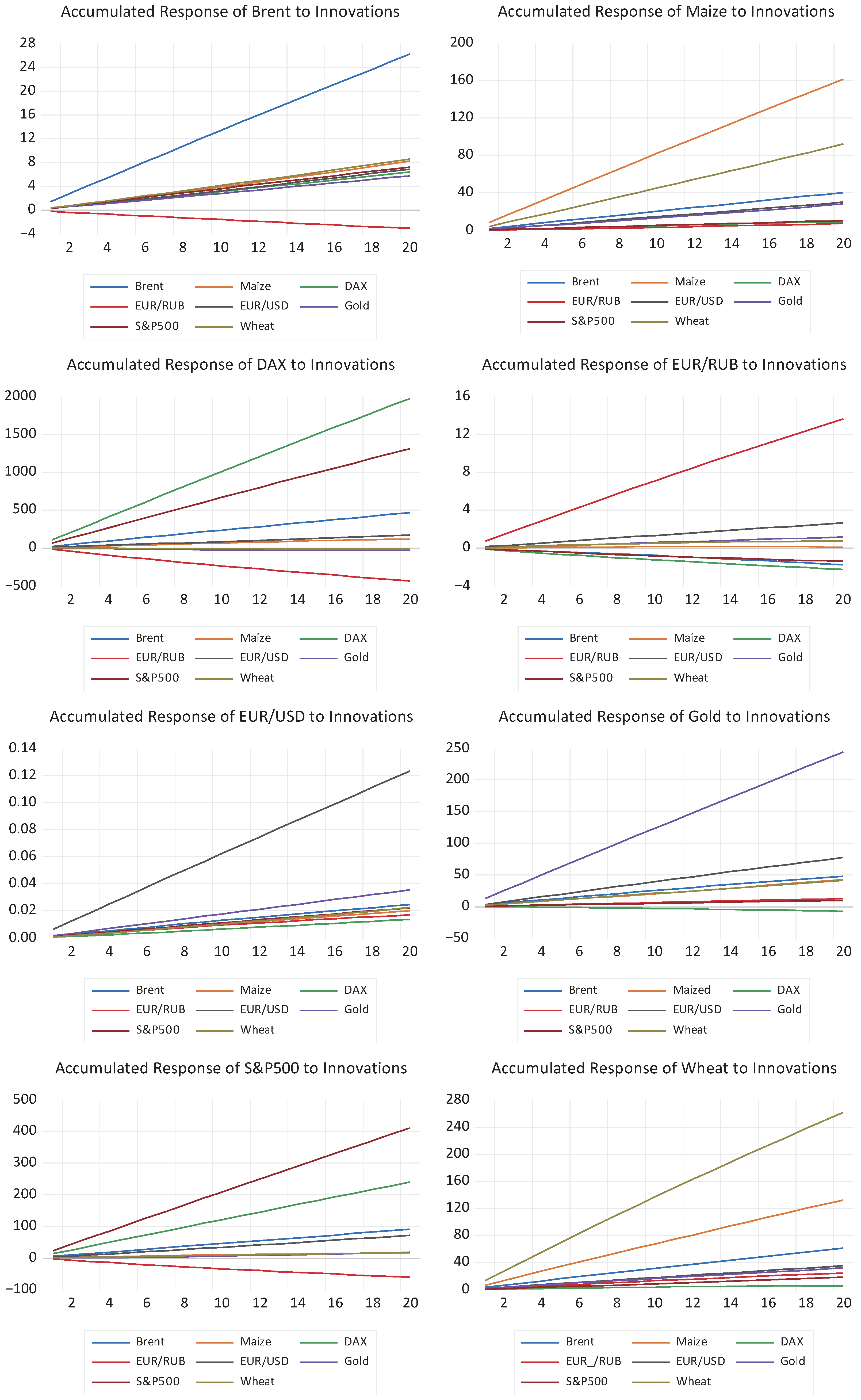
Prior to the implementation of our novel methodology, we employed impulse response analysis (IRF) based on generalized impulse responses, as well as variance decomposition analysis. These techniques are essential for understanding the dynamics of our Vector Autoregression (VAR) model and for evaluating the impact of economic policies over time.

Generalized impulse responses are a critical step in extending our policy impact analysis. Unlike traditional IRFs, which assume that shocks to each variable are orthogonal, generalized impulse responses allow for correlated shocks. This method is more flexible and realistic, as it acknowledges that economic shocks are often interrelated. By using generalized impulse responses, we can obtain a more accurate depiction of how shocks affect the system, thereby enhancing the robustness of our policy impact assessments.

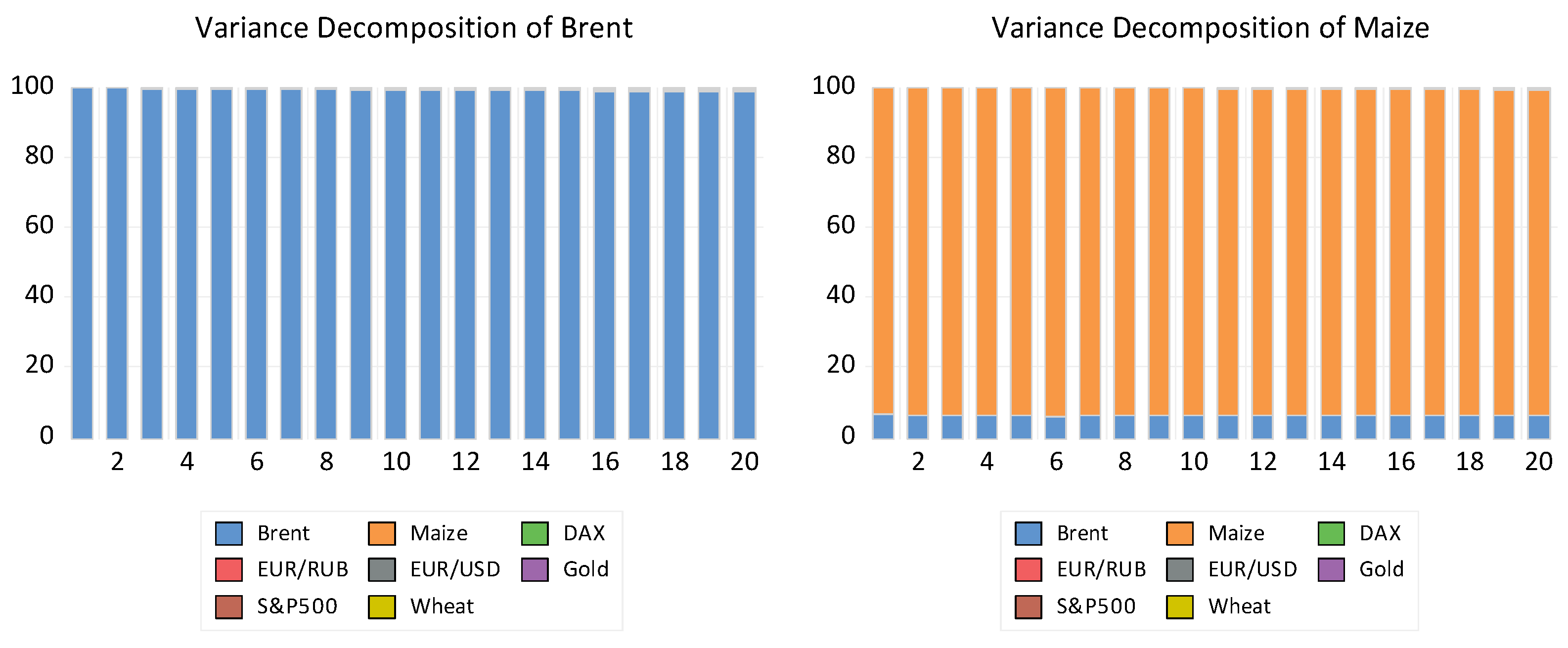
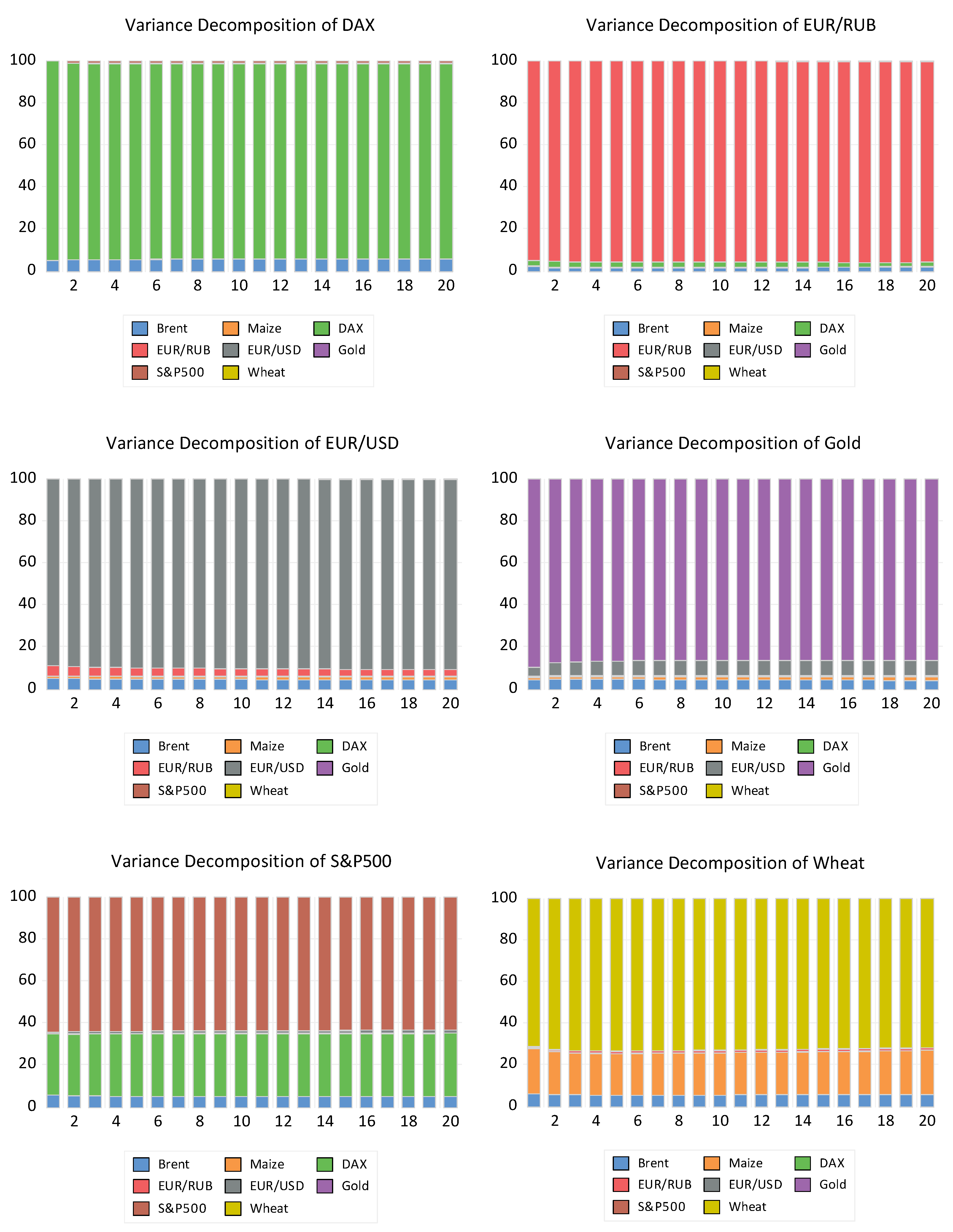
Forecast error variance decomposition (FEVD) was employed to complement the IRF analysis by providing a breakdown of the variance of each variable, listing the contributions made by each shock over different time horizons. This decomposition helps us understand the relative importance of the different shocks in explaining the forecast error variance of each variable. The results of the analysis are provided in the following Figure 1 and Figure 2.

The analysis of these two universally accepted methods—Granger causality and the combination of impulse response function (IRF) and forecast error variance decomposition (FEVD)—demonstrates the interconnectedness of wheat commodity prices with the other variables in the model. Both methods were applied to the same dataset, which includes periods where political events are known to have caused price shocks.

A key distinction between the methodologies lies in the inclusion of first and second lags for wheat in the variance decomposition analysis. The decomposition reveals that previous values of wheat prices account for a substantial portion (over 70%) of the variance, presenting a challenge for isolating the effects of the other variables. While understanding the influence of past values on current prices is important, the primary aim of this study is to explore the connections between the different variables.

The Granger causality method effectively identifies whether one time series can explain another, establishing directional relationships between variables. On the other hand, the IRF-FEVD approach provides a detailed analysis of how shocks to one variable impact others over time, and how much of the forecast error variance for each variable can be attributed to these shocks. However, neither methodology explicitly considers the presence of shocks when assessing the connections between variables.

This limitation underscores the necessity of developing a methodology that can account for these shocks, particularly in scenarios influenced by significant political events. Understanding the direct and indirect effects of such shocks on commodity prices is crucial for a comprehensive analysis of market dynamics and the formulation of effective economic policies.

2.6. Introduction of the Granger Vector Interpretation Method (GVIM)

The output of the Granger causality test typically comprises a table displaying a set of numbers along with their corresponding probabilities. However, when analyzing multiple variables across various periods of the time series, organizing and interpreting the data can be challenging. To address this issue, a novel method is proposed as follows.

Let Y_m denote the time series of the respective variables included in our sample. The period under consideration, T, is divided into n smaller periods, τ_i = [t_i,t_i+1], where 1 ≤ i ≤ n. Assuming all the time series are stationary and included in a VAR model, they undergo the Granger causality test for all periods τ_i. The standard output of the Granger causality test presents a table with each variable Y_j treated as dependent, and the corresponding p-values p_(m,τi) for all other variables Y_m, where m ≠ j and 1 ≤ i ≤ n, are considered independent.

For each pair of Y_j and τ_i (denoted by j, i), m − 1 p-values are displayed. An independent variable is deemed to Granger cause the dependent variable if its p-value p_(m,τi) is lower than the desired significance level, typically 0.05. It is anticipated that the dependent variable in period r may be Granger caused by one set of independent variables, while in period s, the same dependent variable may be Granger caused by a different set of independent variables.

To track the number of variables transitioning from explanatory to non-explanatory for Y_j between periods r and s, the following metric is utilized:

$$f_j\left(Y_m,{\tau }_{r,s}\right)=\left\{\begin{array}{c}0,\mathrm{if}{p}_{m,{\tau }_r}<0.05\mathrm{and}{p}_{m,{\tau }_s}<0.05\mathrm{or}{p}_{m,{\tau }_r}>0.05\mathrm{and}{p}_{m,{\tau }_s}>0.05\\ 1,\mathrm{if}{p}_{m,{\tau }_r}<0.05\mathrm{and}{p}_{m,{\tau }_s}>0.05\mathrm{or}{p}_{m,{\tau }_r}>0.05\mathrm{and}{p}_{m,{\tau }_s}<0.05\end{array}\right.$$

(3)

and form the N_j values according to Equation (4).

$$N_j={\sum }_{m=1,m\ne j}^n{f}_j\left(Y_m,{\tau }_{r,s}\right)$$

(4)

The values of N_j are assembled into the “Variable Transition Vector” (VTV), ${\overrightarrow{u}}_{{\tau }_r,{\tau }_s}$ = (N₁, N₂, …, N_m), representing a comparison between the selected periods r and s. The magnitude of the vector $\left|{\overrightarrow{u}}_{{\tau }_r,{\tau }_s}\right|$ is then calculated. A value of 0 indicates that the independent variables, which were explanatory for the dependent variables in period τ_r, remain unchanged in period τ_s. Conversely, in the scenario where the VTV is at its maximum amplitude, all variables transition from being explanatory in period τ_s to non-explanatory in period τ_r.

Comparing the amplitudes of the VTV values, $\left|{\overrightarrow{u}}_{{\tau }_r,{\tau }_s}\right|$ and $\left|{\overrightarrow{u}}_{{\tau }_k,{\tau }_l}\right|$, provides insight into the changes in the underlying conditions affecting the relationships among the selected variables. If $\left|{\overrightarrow{u}}_{{\tau }_r,{\tau }_s}\right|>\left|{\overrightarrow{u}}_{{\tau }_k,{\tau }_l}\right|$, it suggests a potentially significant alteration in the conditions, leading to increased instability and/or volatility between periods r and s compared to periods k and l.

The VTV values reflect the changes across different pairs of periods, encompassing all variables in the set for all possible pairs of n periods, $\left(\genfrac{}{}{0pt}{}{n}{2}\right)=w$. In certain cases, comparing a specific period with the entire time range T can be beneficial. Therefore, the following function can also be employed:

$$f_j\left(Y_m,{\tau }_i\right)=\left\{\begin{array}{c}0,\mathrm{if}{p}_{m,{\tau }_r}<0.05\mathrm{and}{p}_{m,T}<0.05\mathrm{or}{p}_{m,{\tau }_r}>0.05\mathrm{and}{p}_{m,T}>0.05\\ 1,\mathrm{if}{p}_{m,{\tau }_r}<0.05\mathrm{and}{p}_{m,T}>0.05\mathrm{or}{p}_{m,{\tau }_r}>0.05\mathrm{and}{p}_{m,T}<0.05\end{array}\right.$$

(5)

and N_j values using Equation (3) are calculated to form the respective VTVs.

The minimum value of $\left|{\overrightarrow{u}}_{{\tau }_i,T}\right|$, for i = 1…n, suggests that period ${\tau }_i$ closely explains the total period T, since the variable demonstrates the minimum transition between explanatory and non-explanatory.

Another application of the VTV is where N is calculated with Equation (5) for all single Y_m variables in the sample.

$$N_i=\sum _{\begin{array}{c}r,s=1\\ r\ne s\end{array}}^n{f}_j\left(Y_m,{\tau }_{r,s}\right)$$

(6)

As per the process followed for the formation of VTV ${\overrightarrow{u}}_{{\tau }_r,{\tau }_s}$, a new VTV ${\overrightarrow{v}}_i$ = (N₁, N₂, …, N_w) is created, to provide a measure for the behavior of all Y_m variables in different periods. Like $\left|{\overrightarrow{u}}_{{\tau }_i,T}\right|$, $\left|{\overrightarrow{v}}_i\right|$ is a quantitative measure of the change in the explanatory variables of a dependent variable in different periods.

Both expressions of the VTV form the same Variable transition array as follows:

$A_{{\overrightarrow{u}}_{{\tau }_r,{\tau }_s}}={[{\overrightarrow{u}}_{{\tau }_1,{\tau }_2},{\overrightarrow{u}}_{{\tau }_2,{\tau }_3},\dots {\overrightarrow{u}}_{{\tau }_{w-1},{\tau }_w}]}^{{\rm T}}$ = [${\overrightarrow{v}}_1,{\overrightarrow{v}}_2,\dots {\overrightarrow{v}}_m]$ =$A_{{\overrightarrow{V}}_m}$, as demonstrated in Table 7 below.

3. Results

The breakpoint analysis was performed using the Eviews version 12 software suite, encompassing four distinct date ranges: one covering the entire available dataset from 1/1/2013 to 31/8/2022 (3530 observations), another comprising the first unrest period spanning from 1/1/2013 to 31/12/2014 (730 observations), followed by a period from 1/1/2015 to 31/12/2018 (1481 observations), and finally from 1/1/2019 to 31/8/2022 (1339 observations). The results of the analysis are detailed in Table 4, which presents the date of the breakpoint along with the corresponding t-statistic value, serving as a metric for the intensity of the event at the breakpoint.

The suitability of wheat as the primary indicator for assessing the impact of military actions in the region is evident, given its distinctive response pattern, which is closely aligned with war-related events. As detailed in Section 2, the analysis identifies the most significant breakpoint within a specified period. For wheat, for the timeframe from 2013 to 2022, the pivotal breakpoint aligns precisely with the onset of war in 2022. Similarly, within the 2013 to 2015 timeframe, the most critical breakpoint occurs in 2014, coinciding with the events in Crimea. Conversely, maize (corn) exhibits dissimilar behavior, possibly due to its lesser significance in the perceptions of key market players and the general public compared to wheat.

The analysis underscores that wheat prices have experienced notable shocks corresponding to Russian actions against Ukraine for both instances within the study period. Notably, wheat demonstrated sharper price volatility (breakpoint) compared to the COVID-related shock observed across most other analyzed indicators. Fluctuations in wheat prices are influenced by market supply and demand dynamics, with expectations regarding supply playing a pivotal role, particularly during periods of uncertain physical commodity delivery.

The breakpoints observed for wheat prices correspond precisely with two major events: the outbreak of unrest in Ukraine in May 2014 following the Russian occupation of Crimea, and in March 2022, shortly after the Russian invasion of Ukraine for the second time in the 21st century. Additionally, the EUR/RUB exchange rate demonstrates analogous behavior to the commodity in question, with the shock recorded on the same date, specifically March 9th. This similarity suggests a connection to sanctions and limitations imposed by the EU in the aftermath of the invasion, despite most wheat contracts being negotiated in USD.

During the COVID outbreak, market-oriented indices and gold commodity prices also experienced significant shocks. All these shocks have been reflected by the breakpoint unit root tests implemented, as well as by other tests concerning white noise criteria for residuals or shock terms.

Results of the Implementation of the GVIM Method

The time stamps used for the GVIM method are the same as those used for the breakpoint analysis—t₁, 1/1/2013; t₂, 31/12/2014; t₃, 1/1/2015; t₄, 31/12/2018; t₅, 1/1/2019; and t₆, 31/8/2022—forming periods ${\tau }_1$ = (t₁,t₂), ${\tau }_2$ = (t₃,t₄), ${\tau }_3$ = (t₅,t₆), and T = (t₁,t₆).

The Y_m values are Y₁ for wheat, Y₂ for maize, Y₃ for gold, Y₄ for brent, Y₅ for EUR/USD, Y₆ for EUR/RUB, Y₇ for the DAX, and Y₈ for the S&P500. Applying Equation (3) to all Y_j, we calculate N_j sum values. The values for the comparison of ${\tau }_i$, i = 1, 2, 3 periods with T, are calculated with the application of Equation (3). The results are shown in

Table 6. Granger causality test and respective $p_{m,{\tau }_i}$ values.

	Dependent Yj	Wheat	Maize	Gold	Brent	EUR/USD	EUR/RUB	DAX	S&P500
Independent Ym m≠j
Wheat			0.367	0.303	0.403	0.229	0.528	0.245	0.785
			0.475	0.904	0.708	0.398	0.734	0.310	0.942
			0.769	0.006 *	0.000 *	0.239	0.271	0.000 *	0.839
			0.042 *	0.616	0.003 *	0.205	0.001 *	0.392	0.649
Maize		0.907		0.124	0.666	0.136	0.212	0.527	0.845
		0.204		0.577	0.832	0.815	0.981	0.219	0.353
		0.151		0.187	0.082	0.528	0.889	0.086	0.997
		0.652		0.233	0.305	0.148	0.138	0.047 *	0.495
Gold		0.832	0.573		0.515	0.707	0.418	0.299	0.008 *
		0.326	0.826		0.783	0.541	0.493	0.692	0.413
		0.475	0.238		0.631	0.000 *	0.004 *	0.073	0.834
		0.011 *	0.518		0.668	0.000 *	0.479	0.804	0.359
Brent		0.333	0.591	0.748		0.271	0.814	0.613	0.819
		0.466	0.063	0.277		0.131	0.096	0.012 *	0.134
		0.005 *	0.421	0.483		0.496	0.000 *	0.214	0.430
		0.000 *	0.008 *	0.689		0.079	0.159	0.885	0.033 *
EUR/USD		0.007 *	0.002 *	0.067	0.589		0.569	0.534	0.411
		0.421	0.859	0.003 *	0.097		0.422	0.101	0.304
		0.118	0.881	0.047 *	0.566		0.289	0.086	0.192
		0.049 *	0.996	0.014 *	0.475		0.189	0.831	0.000 *
EUR/RUB		0.923	0.427	0.897	0.781	0.688		0.007 *	0.002 *
		0.671	0.030 *	0.450	0.055	0.114		0.134	0.128
		0.021 *	0.019 *	0.645	0.868	0.000 *		0.054	0.362
		0.472	0.440	0.001 *	0.000 *	0.329		0.288	0.058
DAX		0.015 *	0.613	0.752	0.732	0.063	0.001 *		0.647
		0.851	0.191	0.706	0.681	0.202	0.714		0.805
		0.515	0.012 *	0.802	0.922	0.027 *	0.957		0.325
		0.000 *	0.031 *	0.157	0.701	0.014 *	0.002 *		0.000 *
S&P500		0.062	0.852	0.885	0.875	0.763	0.419	0.000 *
		0.968	0.437	0.738	0.011 *	0.532	0.636	0.000 *
		0.627	0.396	0.407	0.232	0.000 *	0.266	0.000 *
		0.821	0.717	0.911	0.180	0.999	0.034 *	0.474

Note: ${\tau }_1$, ${\tau }_2$, ${\tau }_3$, and T periods are in respective order; * p-value < 0.05 indicates an explanatory variable according to Granger causality theory.

and

Table 7. Variable Transition Array, vectors, and amplitudes *.

Comparison between Periods		Wheat	Maize	Gold	Brent	EUR/USD	EUR/RUB	DAX	S&P500	VTV	$\left|{\overrightarrow{\mathit{u}}}_{{\mathit{\tau }}_{\mathit{r}},{\mathit{\tau }}_{\mathit{s}}}\right|$
${\tau }_1$	${\tau }_2$	2	2	1	1	0	1	2	2	(2,2,1,1,0,1,2,2)	4.36 *
${\tau }_2$	${\tau }_3$	2	1	1	2	4	2	2	0	(2,1,1,2,4,2,2,0)	5.83 *
${\tau }_1$	${\tau }_3$	4	3	2	1	4	3	2	2	(4,3,2,1,4,3,2,2)	7.94 *
VTV		(2,2,4)	(2,1,3)	(1,1,2)	(1,2,1)	(0,4,4)	(1,2,3)	(2,2,2)	(2,0,2)
$\left|{\overrightarrow{v}}_i\right|$		4.90 *	3.74 *	2.45 *	2.45 *	5.66 *	3.74 *	3.46 *	2.83 *
${\tau }_1$	Τ	5	2	3	2	1	3	3	3	(5,2,3,2,1,3,3,3)	8.37 *
${\tau }_2$	Τ	3	2	1	1	1	4	3	2	(3,2,1,1,1,4,3,2)	6.71 *
${\tau }_3$	Τ	1	1	2	0	1	3	3	0	(1,1,2,0,1,3,3,0)	5.00 *
VTV		(5,3,1)	(2,2,1)	(3,1,2)	(2,1,0)	(1,1,1)	(3,4,3)	(3,3,3)	(3,2,0)
$\left|{\overrightarrow{v}}_i\right|$		5.92 *	3.00 *	3.74 *	2.24 *	1.73 *	5.83 *	5.20 *	3.61 *

Note: The numbers in cells indicate number of variables transitioning from explanatory to non-explanatory and vice versa, across the periods shown in the first column. The resulting vectors ${\overrightarrow{u}}_{{\tau }_r,{\tau }_s}$ and ${\overrightarrow{v}}_i,$ with their amplitudes, are also included in the table. The visual representation of the phenomenon is shown in Figure 3. Numbers with * indicate vector amplitudes.

.

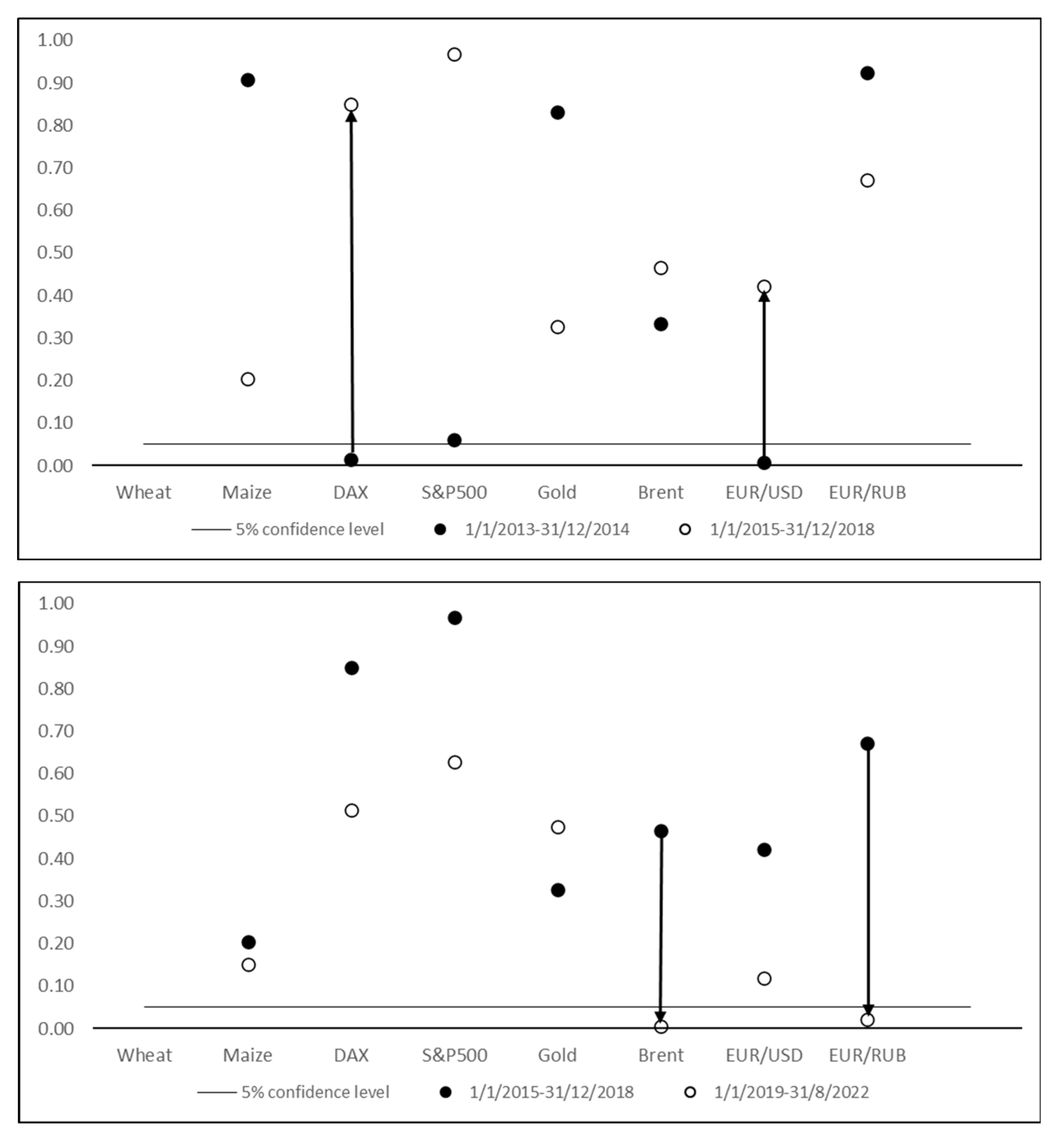
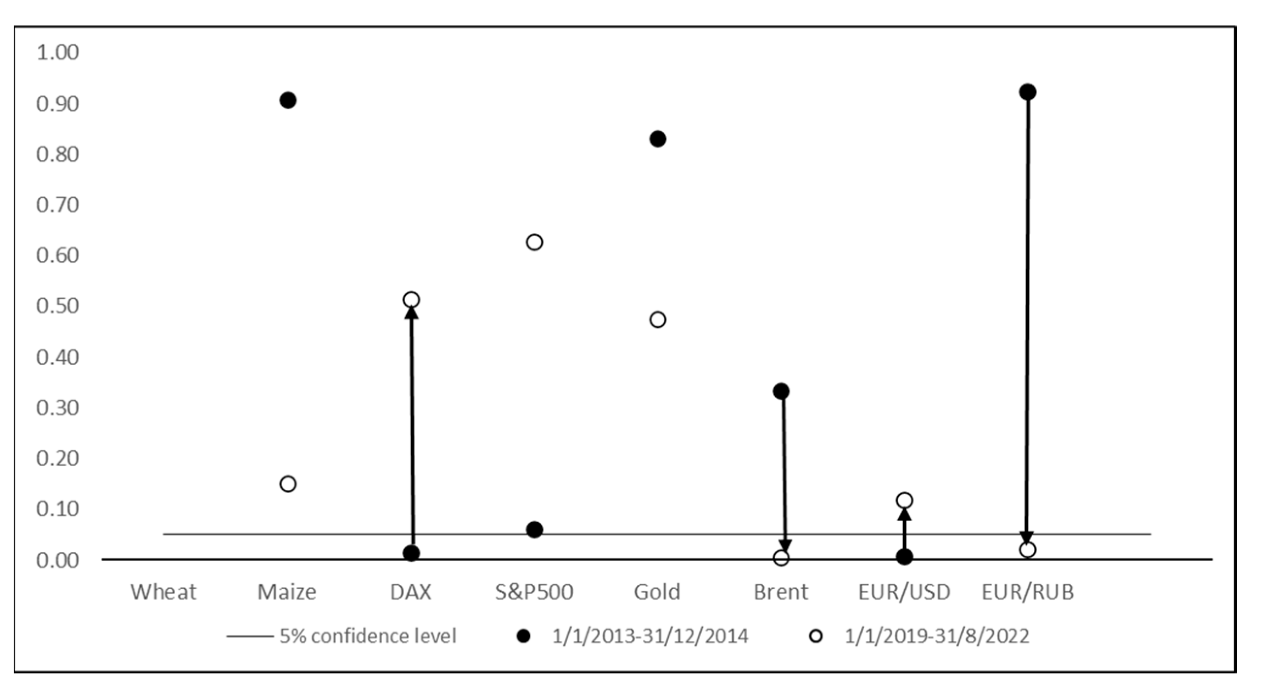
In Figure 3, the graphical representation of points N is demonstrated. The transition of the Y variables to different sides of the line representing the 5% significance level between periods ${\mathit{\tau }}_{\mathit{i}}$ is shown.

4. Discussion

Post implementation of the Granger Vector Interpretation Method (GVIM), it becomes evident that the selected variables for this study are intricately linked to the geopolitical events of the examined periods. Comparing $\left|{\overrightarrow{u}}_{{\tau }_r,{\tau }_s}\right|$ for period τ₁ to period τ₂, the VTV value is small, indicating minimal changes in the independent variables Granger causing the dependent variables between these periods. Conversely, when period τ₁ is compared to period τ₃, the VTV value is larger, signifying a substantial transition in variables. This suggests a shift in market and political conditions impacting the behavior of indices, commodity prices, and exchange rates. Despite both periods encompassing unrest in the Russian–Ukrainian border region, other significant events altered the interdependency of variables.

The significant shocks in the global economy during period τ₃ are supported by the large VTV values when comparing this period with the others. Moreover, when τ₃ is compared to the entire period T, the VTV value is small, indicating that the events in τ₃ had a pervasive influence throughout the entire period, as expected due to the occurrence of both COVID and war.

The maximum VTV value for $\left|{\overrightarrow{v}}_i\right|$ is 12,12 (three pairs of time periods with seven variables would form vector (7, 7, 7)), which would be obtained in the extreme event that all the variables in the VAR model shifted from explanatory to non-explanatory and vice versa. Examining the individual variables reveals that wheat exhibits a notably large VTV $\left|{\overrightarrow{v}}_i\right|$ value of 4.90, second only to the EUR/USD exchange rate when comparing periods τ₁, τ₂, and τ₃. This underscores the strong connection between wheat and the events of the periods, indicating the commodity’s sensitivity to political decisions and actions. The GVIM output highlights the significant fluctuations in economic indicators linked to wheat over time, particularly near shocks, posing challenges for predictive models.

Furthermore, when comparing pairs of periods within the entire sample period T, the VTV score for wheat surpasses that of all other indicators at 5.92. Similar to the above maximum estimation for |7, 7, 7|, this underscores the distinct behavior of wheat prices compared to the rest of the set. The strong influence of events in τ₃ is evident, as indicated by the minimal difference between this period and the entire sample.

Indeed, the proposed Granger Vector Interpretation Method (GVIM) can be readily automated, making it suitable for analyzing large sets of variables efficiently. By automating the process, researchers can streamline the analysis of complex datasets, enabling them to uncover meaningful insights and relationships among variables more effectively.

Automation would involve developing software that integrates the GVIM methodology, allowing users to input their datasets and specify the relevant parameters for analysis. The software would then perform the necessary calculations and generate outputs, such as Variable Transition Vectors (VTVs) and associated metrics, to facilitate interpretation and decision making.

Certainly, expanding the proposed methodology to incorporate variable arrays instead of vectors could enhance the dimensional interpretation of the results and pave the way for further research avenues. By extending the analysis to variable arrays, researchers could capture more nuanced relationships and interactions among multiple variables, offering a richer understanding of complex systems.

Variable arrays would allow researchers to explore higher-dimensional relationships among variables, offering insights beyond simple pairwise interactions. This approach could involve organizing variables into multidimensional arrays or tensors, where each dimension represents a different aspect or characteristic of the data.

In the future, the GVIM method has the potential to serve as a valuable measure of variation or change, aiding forecasting methods that are influenced by fluctuations in the variables under study. By quantifying the transitions of variables from being explanatory to non-explanatory and vice versa, GVIM can provide insights into the dynamics of the underlying relationships among variables over time.

5. Conclusions

During the course of this study, the behavior of market indices, particularly agricultural commodity prices, was meticulously researched across different time periods. This included periods marked by political shocks, such as aggressive actions between nations, which pose significant challenges for determining the interlinkages among prices. Understanding these interconnections is crucial for various market participants and policymakers. To address these challenges, we proposed the application of the novel GVIM (Granger Vector Interpretation Method), described above.

Political events can cause substantial volatility in commodity prices, and these fluctuations can have cascading effects on other economic indices. For example, region-specific commodities, such as wheat, have shown a strong response to political events, which is consistent with similar estimates found in the existing literature (Hudecová and Rajčániová 2023). The GVIM method enhances our ability to quantify these relationships by providing a fast and quantitative representation of shifts in the explanatory variables.

As we mentioned above, the scientific methods used to determine if the selected variables in a model are interpreted correctly include the impulse response function (IRF) and Granger causality. Although both methods yield qualitatively similar results, IRF is a method that requires significant time and expertise to implement, as the choice of variables and their order in the model are crucial. Granger causality is clearly simpler and quicker.

The GVIM method simplifies the traditionally complex task of interpreting the outputs from multiple Granger causality tests. It does so by converting these results into sets of numbers that indicate the transitions from Granger-causing to non-Granger-causing variables. This approach makes the method accessible even to market participants who may lack extensive mathematical backgrounds. The ability to quickly interpret these shifts is invaluable for traders, speculators, and hedge funds, especially in times of crisis.

Wider adoption of the proposed GVIM method could prove highly beneficial to key market players and decision makers. For market participants, understanding the changes in the connections among variables is essential for their strategies, whether for hedging, investing, or speculation. The GVIM method would provide them with a robust tool to monitor and react to those changes effectively. It would help in identifying when traditional models may no longer be valid due to shifts in underlying relationships caused by political shocks.

On the other hand, policymakers could use the GVIM method to gain insights into the implications of price shocks. By understanding how these shocks affect commodity prices and other economic indices, they could better forecast the effects of policy changes and geopolitical events. This understanding could inform more effective policy responses to stabilize markets and mitigate adverse impacts on the economy.

The practical implementation of the method should benefit interested parties by initially acknowledging the possibility that shocks can cause changes in the interlinkages among variables. This understanding is crucial for accurately interpreting the dynamic relationships within a dataset. To effectively manage this, the first step is to confirm the presence of shocks through a breakpoint analysis. A breakpoint analysis helps identify the specific points in time where significant shifts in causal effects are expected. Once these breakpoints are established, they provide a clear indication of when the relationships between variables might have changed due to external shocks.

By comparing causal effects before and after these identified shocks, analysts can gain insights to how the dynamics of the variables have evolved over time. This comparison allows for a more refined understanding of the underlying processes and helps in adjusting the models used for analyzing the behavior of a variable.

Incorporating these changes into the models ensures that they reflect the new status quo of causal effects. This adjustment is essential for maintaining the accuracy and reliability of the models for predicting future behaviors and responses to similar shocks. Ultimately, this approach enhances the robustness of the analysis, providing valuable information for policymakers, market analysts, and other stakeholders who rely on these models to make informed decisions. This methodological framework not only improves the precision of economic models but also enhances their applicability in real-world scenarios where shocks are common and often substantial.

In conclusion, the GVIM method represents a significant advancement in the analysis of economic indices and commodity prices in the context of political events. Its simplicity and quantitative clarity make it a valuable tool for both market participants and policymakers. By adopting this method, they can better navigate the complexities introduced by geopolitical shocks and make more informed decisions in their respective fields.