1. Introduction
The mechanics of derivative pricing theory have fundamentally changed in the aftermath of the global financial crisis (GFC) in 2008. Following the GFC, it was uncovered that specific assumptions underpinning classical derivative pricing theory, such as the existence of a unique risk-free rate at which parties can borrow and lend in the Black–Scholes (BS) model by
Black and Scholes (
1973), were not necessarily realistic. To address this limitation,
Piterbarg (
2010) derived a theoretical pricing framework from first-principles that relaxes the assumption on the existence of a unique risk-free rate and incorporates the effects of collateral on the price of a financial derivative.
In addition to the fundamental changes to derivative pricing theory post the GFC, the rapid advancement of technology has seen research focused on machine learning techniques across numerous financial disciplines grow exponentially in recent years. This is primarily driven by the ease with which these techniques can be developed and implemented using tools and information that are widely available.
Modern day financial machine learning literature studies, such as the literature review by
Ruf and Wang (
2020), have highlighted the extensive exploration of these techniques in the pricing, hedging, and risk management of derivative securities. The majority of the literature, as mentioned by
Ruf and Wang (
2020), has been solely focused on approximating the prices of financial derivatives. Research on the hedging and risk management of financial derivatives has been largely limited in comparison.
The aim of this paper is to contribute to the existing literature by showing that ANNs can be trained to approximate the option price sensitivities of both the BS and the Piterbarg models in a real-world setting. Multi-curve frameworks, such as the Piterbarg model, have become increasingly relevant after the GFC, given that the effects of collateral on the price of financial derivatives are considered. Furthermore, the out-of-sample performance of the optimized ANNs will be evaluated using option price data sourced from the South African market. The South African market was specifically chosen given that there is a gap in the current literature on the real-world financial applications of machine learning techniques. The majority of related studies have either focused on more developed and liquid markets or considered simulated data only.
The structure of this paper is as follows:
Section 2 provides a review of recent and relevant literature.
Section 3 focuses on the theoretical frameworks of the BS and Piterbarg models.
Section 4 outlines the ANN architecture and configurations as well as the training and test data used.
Section 5 discusses the results, which is followed by the concluding remarks in
Section 6.
2. Literature Review
The use of machine learning techniques in financial applications is well-documented in the literature and continues to be a field of keen interest. In this section, a review of relevant literature is provided.
In the seminal paper by
Hutchinson et al. (
1994), a new paradigm in the pricing and hedging of financial derivatives through the use of machine learning techniques was explored. It was argued that the effectiveness of classical approaches, such as the BS model, used in the pricing and hedging of financial derivatives depends on the ability to model the dynamics of the underlying asset process. It was proposed that instead of theorizing more complex models to capture the dynamics of a market, simple data-driven approaches, such as ANNs, can be used to learn the dynamics of the underlying asset process as well the relation between the underlying asset process and other observed market variables to the price of a financial derivative.
The financial applications of machine learning techniques were further explored in the breakthrough research by
Buehler et al. (
2019), where a framework for the hedging of financial derivatives reflective of the various intricacies of real-world markets was proposed. To address the deficiencies present in traditional market models, a deep hedging framework was proposed which modeled trading decisions used in hedging strategies as ANNs. Furthermore, since the deep hedging framework is data-driven, there is no need to explicitly calculate the option price sensitivities using traditional derivative pricing models, since these risk measures are implied within the deep hedging strategy.
The use of machine learning techniques in approximating not only the prices of financial derivatives but also the respective option price sensitivities has been explored in more recent research. In
Ratku and Neumann (
2022), it was shown that a deep feed-forward ANN optimized to approximate the pricing function of the
Heston (
1993) stochastic volatility model for European options could also be used to accurately approximate the respective option price sensitivities. The conclusions drawn from this study were based on a data set that was artificially generated by uniformly sampling data from a range of input parameters.
In a similar study,
Umeorah et al. (
2023) approximated the closed-form solutions to the option price and option price sensitivities of barrier options using a feed-forward ANN. The performance of the ANN was further compared to other techniques, such as random forest and polynomial regression. Given a simulated data set, it was found that ANNs provide an efficient and effective alternative to complex existing approaches for pricing barrier options and that an optimized ANN outperforms the other machine learning techniques considered in the study.
A general shortcoming observed from the literature considered in this paper is the fact that the numerical applications of these studies are often solely based on simulated or artificially generated data sets. This is mostly due to a lack of sufficient option price data needed to train data-driven techniques, such as ANNs. As a result, the out-of-sample performance of machine learning techniques in real-world applications, especially in illiquid financial markets, has received less attention. Additionally, a focus is often placed on classical frameworks, such as the BS model, which do not consider the effects of collateral on the price of derivative securities.
Therefore, this paper aims to address these gaps in the existing literature by evaluating the out-of-sample performance of ANNs in approximating the option price sensitivities in both a classical BS and multi-curve framework, such as the Piterbarg model, using option price data sourced from the South African market. The methodology of this paper is outlined in the next section.
3. Methodology
In this section, a brief overview is provided on the theory underpinning the BS and Piterbarg models. It is, however, useful to first define the respective option price sensitivities that form the basis of this paper.
3.1. Option Greeks
Option price sensitivities or Greeks are extensively used by financial practitioners, such as traders, to monitor and manage the risk in a trading position, where each option Greek as described by
Hull (
2009) is used to capture a specific dimension of risk to a position. More formally, the option Greeks can be seen as the partial derivatives of the value of the option with respect to the parameters that the value is derived from. The option Greeks considered in this study based on the definitions by
Leoni (
2014) can be described in a general sense ignoring time subscripts as follows:
3.1.1. Delta
Delta
is the sensitivity of the option price
V with respect to changes in the value of the underlying asset
S:
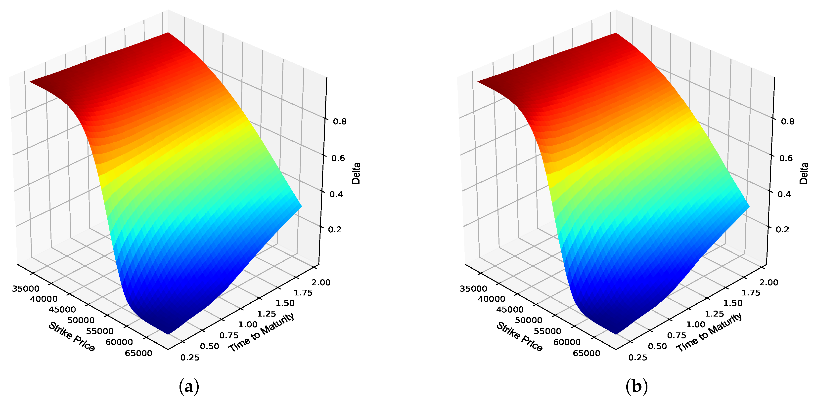
and is the amount of the underlying asset that should be traded to hedge the option position. Delta ranges from 0 to 1 for European call options and from 0 to −1 for European put options. The Delta of an out-of-the-money (OTM) European call option is close to 0 since it is unlikely that the option will be exercised by the holder and close to 1 for an in-the-money (ITM) European call option, therefore requiring a full hedge of the option position.
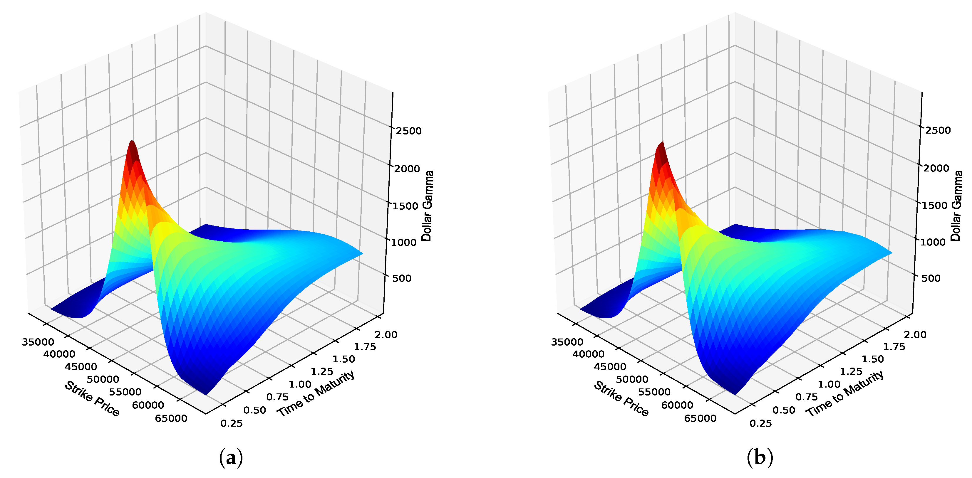
3.1.2. Gamma and Dollar Gamma
Gamma
is a second-order partial derivative and measures the sensitivity of Delta with respect to changes in the value of the underlying asset:
and is positive for both European call and put options. The Gamma of a European call option is largest for at-the-money (ATM) options since Delta is most sensitive around this point, and tends to flatten out for OTM and ITM options. A useful simplification made in this paper to avoid dealing with minuscule or zero-valued outputs when training the ANNs to approximate Gamma is to consider Dollar Gamma
$ throughout this paper which is given by:
3.1.3. Vega
Vega
measures the sensitivity of the option price with respect to changes in the implied volatility
of the underlying asset:
and is positive for both European call and put options. Vega tends to increase as the time to maturity of the option increases, especially for an ATM option given that there is more uncertainty around whether the option will be ITM or OTM at maturity. Vega tends toward zero for ITM and OTM options as the option reaches maturity given that large moves in the underlying price are less likely given the shorter time frame.
3.1.4. Theta
Theta
measures the sensitivity of the option price with respect to changes in the passage of time
t:
and is typically negative for both European call and put options given that an option loses value as it approaches maturity. Theta is greatest (smallest) for an ATM option near maturity and approaches zero for OTM options given that it is less likely for an OTM option to gain value over time.
3.1.5. Rho
Rho
measures the sensitivity of the option price with respect to changes in the interest rate
r:
and is typically viewed as one of the option Greeks of lesser importance given that the value of an option is less sensitive to changes in interest rates compared to changes in the other pricing parameters. This holds true since changes in interest rates are typically small and less frequent. Rho is positive for European call options and negative for European put options. The next section presents the theory underlying the BS model as well as the explicit solutions of the respective option Greeks.
3.2. The Black–Scholes Model
Black and Scholes (
1973), through their seminal paper, introduced the BS model for the valuation of European options under the assumption of a complete and frictionless market. Under these assumptions, the value of a European option only depends on the price of the underlying
S, the time
t, and other known constant variables, such as the strike price
K, the unique risk-free rate
r, and the implied volatility
. The partial differential equation (PDE) for a European call option on a non-dividend paying stock is derived by constructing a self-financing portfolio and is given by:
The closed-form solution to the PDE in Equation (
1) for the value of a European call option at time
t exists and is given by:
where
and
is the cumulative distribution function of the standard normal distribution. Given the closed-form solution for the value of a European call option in Equation (
2), the explicit solutions of the respective option Greeks are given by:
where
is the probability density function of the standard normal distribution and
and
are given by Equations (
3) and (
4).
3.3. The Piterbarg Model
Piterbarg (
2010) introduced an extension to the classical BS model which relaxes the assumption that parties can borrow and lend at a unique risk-free rate. Under the Piterbarg model, the effects of collateral on the price of a financial derivative is incorporated into a valuation framework through the introduction of three deterministic interest rates, namely, the collateral rate
, the repurchase agreement rate
, and the funding rate
, where the following relationship holds:
As stated by
Hunzinger and Labuschagne (
2015) in the context of the inequality in Equation (
5), if a trade is collateralized, then future expected cash flows are discounted off the collateral curve. On the contrary, if a trade is not collateralized, then future expected cash flows are discounted off the funding curve to appropriately reflect the credit riskiness of the trade. This makes intuitive sense given that collateral is used to mitigate counterparty credit risk in over-the-counter (OTC) trades. The Piterbarg PDE, which incorporates the presence of collateral
C is derived by constructing a self-financing portfolio and is given by:
Based on the work by
von Boetticher (
2017), it was shown that a closed-form solution for a zero collateral (ZC) European call option, where no collateral is posted, and a fully collateralized (FC) European call option, where the collateral posted is equal to the value of the derivative, can be derived from the PDE in Equation (
6). If interest rates are assumed to be constant, then it follows that:
and
where
The explicit solutions to the respective option Greeks for ZC and FC European call options assuming constant interest rates based on the derivations by
Labuschagne and von Boetticher (
2017) are presented below. It should be noted that Rho under the Piterbarg model for the purposes of this paper is expressed with respect to the repurchase rate only.
The explicit solutions of the option Greeks considered in this paper for a ZC European call option derived from Equation (
7) are of the form:
Similarly, in the case of an FC European call option, the explicit solutions of the respective option Greeks derived from Equation (
8) are of the form:
where
and
are given by Equations (
9) and (
10). In the next section, the general ANN architecture and configuration is discussed and an overview of the training and test data considered in this paper is provided.
4. Data and Network Architecture
The following section discusses the general ANN architecture and specifications and provides an overview of the procedure to generate artificial option price data for training the ANNs used to approximate the respective option Greeks under the BS and Piterbarg models. This section also elaborates on the construction of an implied volatility surface using option price data from the South African market, which will serve as the test data set to evaluate the out-of-sample performance of the optimized ANNs under the BS and Piterbarg models.
4.1. ANN Architecture and Configuration
In this section, the chosen ANN architecture and hyper-parameter configurations for the BS and Piterbarg option Greek ANNs are discussed. The respective ANNs were implemented in Python using the Keras Application Programming Interface (API) based on TensorFlow 2.0 developed by
Chollet (
2015).
For the purposes of this paper, the ANN architecture and hyper-parameters were configured with an eye toward keeping the ANN structure and hyper-parameter configuration as standard as possible. It is worth mentioning that according to the universal approximation theorem by
Cybenko (
1989) and
Hornik et al. (
1989), a single hidden layer feed-forward ANN with a continuous non-linear activation function can approximate any continuous function. Therefore, as long as the chosen activation functions within a feed-forward ANN are suitable for the problem at hand, a standard ANN structure in terms of the number of hidden layers and neurons per hidden layer will suffice. The general ANN architecture and configurations are outlined in
Table 1.
From
Table 1, it can be seen that the same ANN architecture was applied to approximate each Greek, with only slight differences in the choice of the output activation function. For example, the Delta of a European call option under the BS model is between 0 and 1; therefore, to use the sigmoid function in the output layer helps restrict output values to this desired domain. The Delta of an FC European call option can, however, be slightly greater than 1 due to the fact that a European call option that is fully collateralized is discounted using the collateral rate which is lower than the repurchase agreement rate. The Softplus function is, therefore, an ideal output activation function to ensure that outputs are positive given its non-zero-centered property and not bounded from above. Finally, a linear output activation function was selected for ANNs approximating Theta under both theoretical frameworks due to its zero-centered property which can output negative values that are not restricted to a specific domain. The mean absolute error (MAE) was selected as the loss function when fitting the respective ANNs due to the fact that the MAE is more robust to noisy data when outliers are present in the artificially generated training data. Given the rather noisy artificially generated data and the non-linear profiles of the respective option Greeks, it was observed during the initial testing that the MAE resulted in more stable performance compared to the mean squared error (MSE). The next section provides an overview of the training and test data considered in this paper.
4.2. Training and Test Data
It is a known fact that option price data are scarce in emerging markets, such as South Africa, due to these markets being illiquid compared to other more developed markets. To address this limitation, option price data were artificially generated to train and validate the ANNs. Artificial data sets consisting of 2,000,000 samples were generated by uniformly sampling data from a wide range of input parameter ranges. The parameter ranges used to generate data for training the BS ANN Greeks are outlined in
Table 2.
Similarly, the training data for the Piterbarg ANN Greeks were generated from the parameter ranges outlined in
Table 3.
From the respective artificially generated data sets, 80% of the generated samples were used as the training set, and the remaining 20% of the generated samples were used as the validation set. Given that spot and strike prices are required to calculate the sensitivity values under the BS and Piterbarg models to serve as the output sets, the underlying spot price of the JSE Top 40 Index equal to R51 564.09 as at 9 April 2019 was used to convert the moneyness ratio (
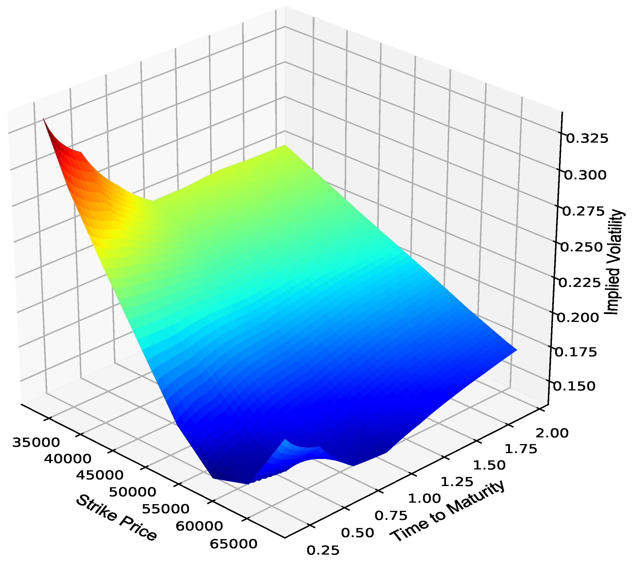
) into strike prices. The test set used to evaluate the out-of-sample performance of the optimized ANN Greeks comprised JSE Top 40 European call option price data obtained from the JSE. The option price data consisted of volatility skews from which an implied volatility surface was constructed using linear interpolation in the strike dimension, and linear variance interpolation in the maturity dimension. This resulted in a granular surface comprising 10,000 implied volatility estimates, as shown in
Figure 1.
It is further assumed that the same constructed implied volatility surface is used to evaluate the out-of-sample performance of the optimized ANN Greeks under both the BS and Piterbarg models, given that ZC and FC option price data are not available within the South African market. Constant interest rates are further assumed with , , and , which allows for the Piterbarg option Greeks to be calculated analytically. The same underlying index spot price as at 9 April 2019 used for the training and validation sets was also used as an input to the test set. The out-of-sample performance of the optimized ANN Greeks compared to the explicit solutions of the option Greeks under the BS and Piterbarg model is discussed in the next section.
5. Results
This section provides an overview of the results obtained by deploying the optimized ANN Greeks to an out-of-sample test set to numerically approximate the respective option Greeks under both the BS and Piterbarg model. This section consists of two parts: the first part focuses on the results obtained under the BS model, whereas the second part focuses on the ZC and FC results under the Piterbarg model.
5.1. Numerical Results: Black–Scholes Option Greeks
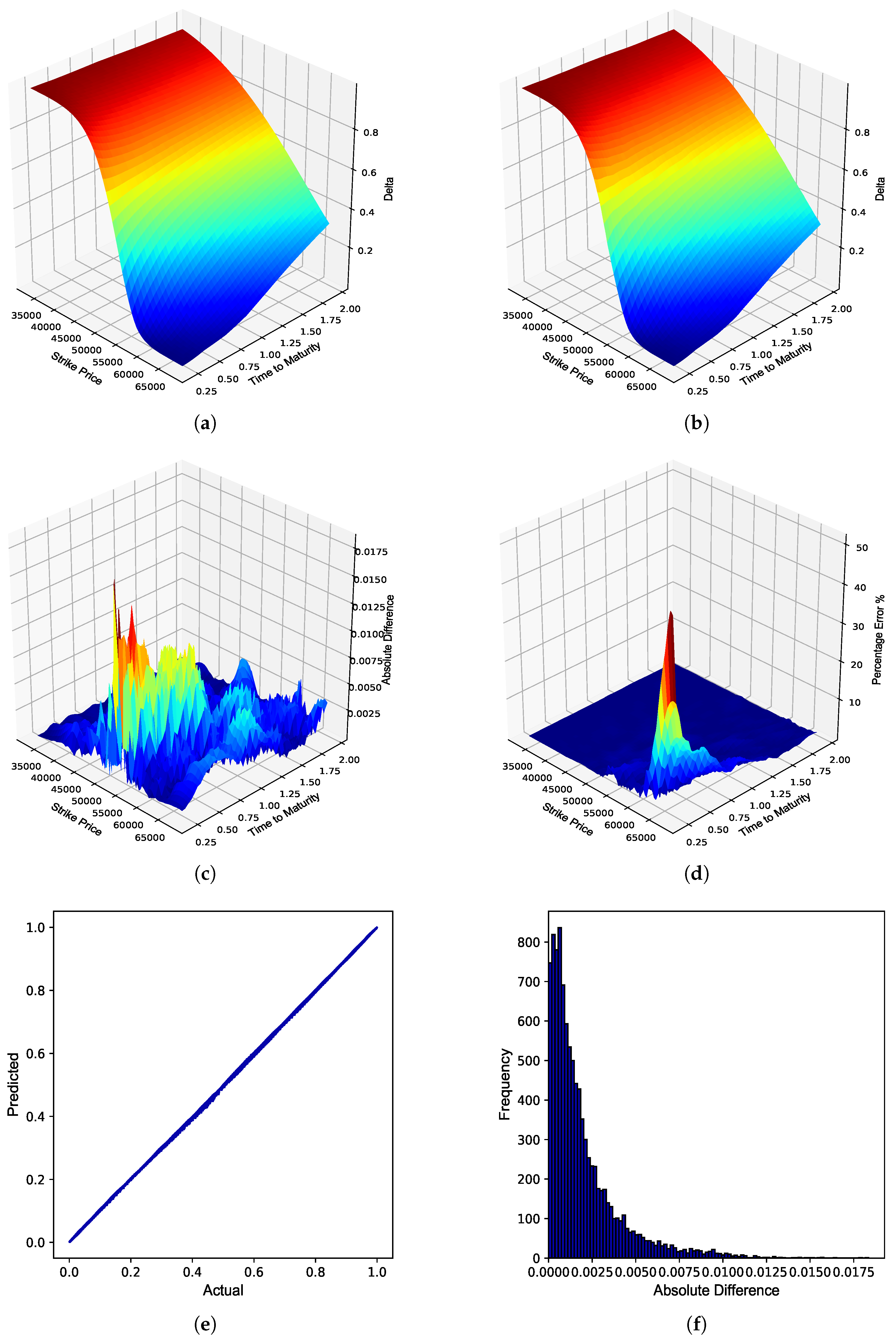
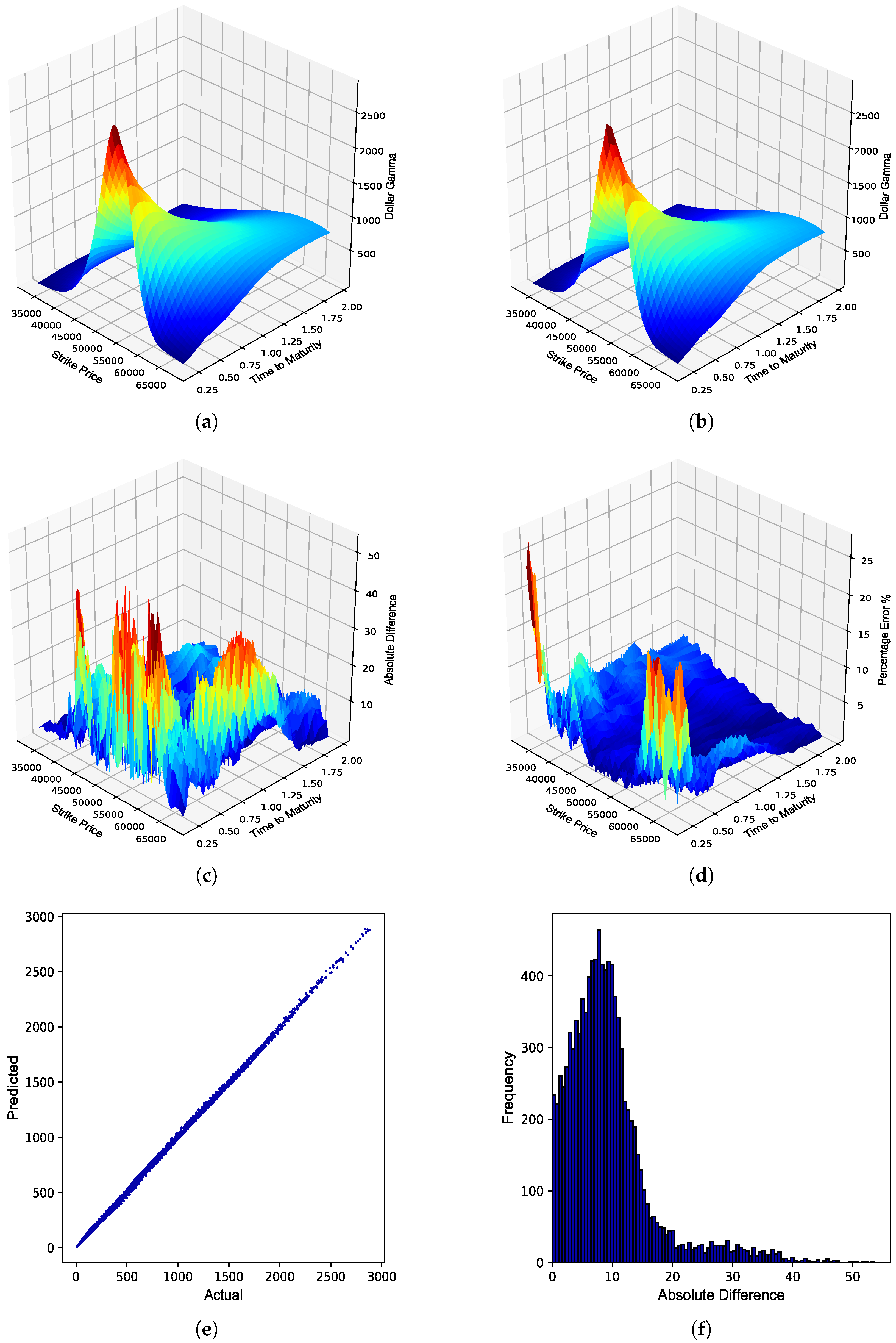
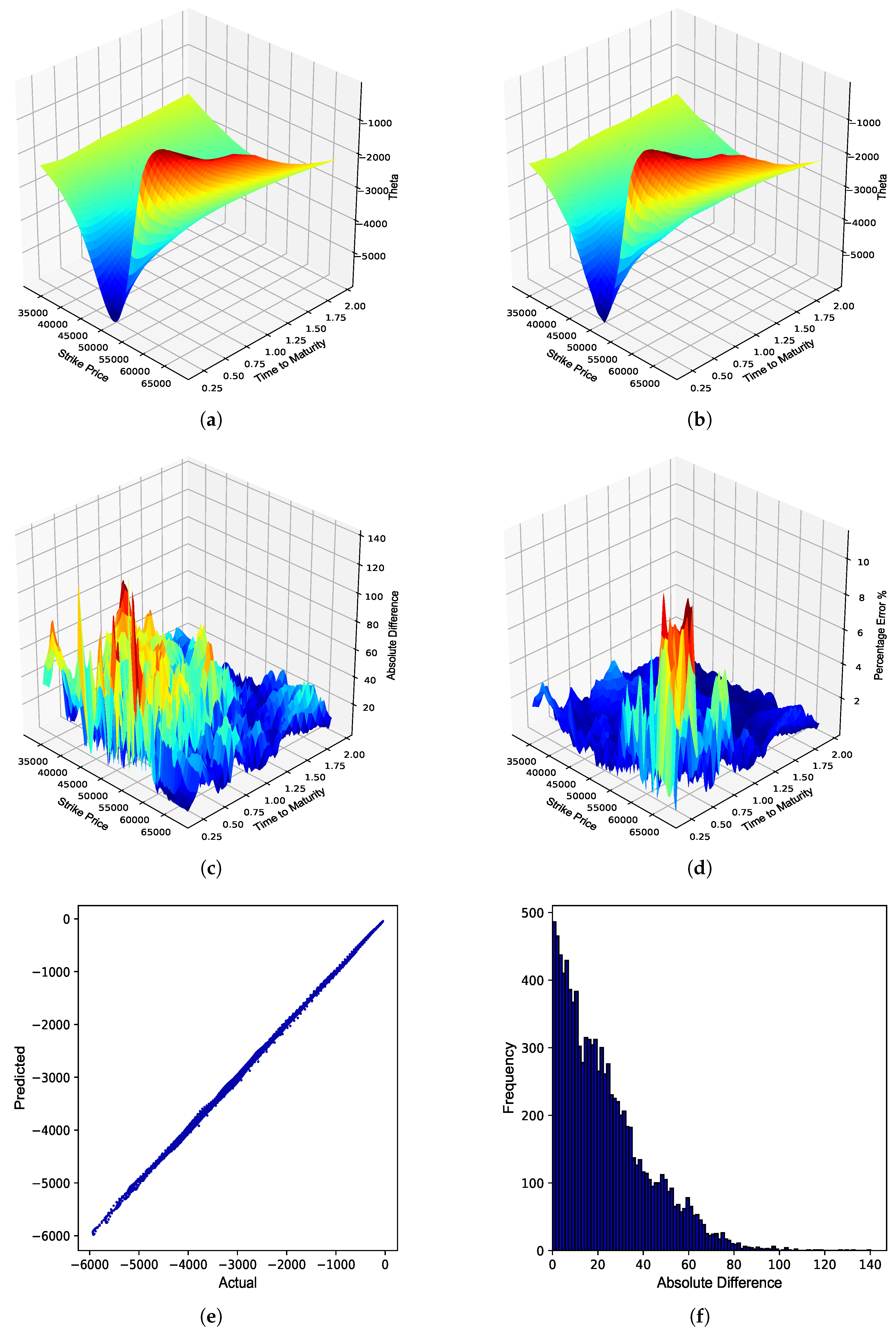
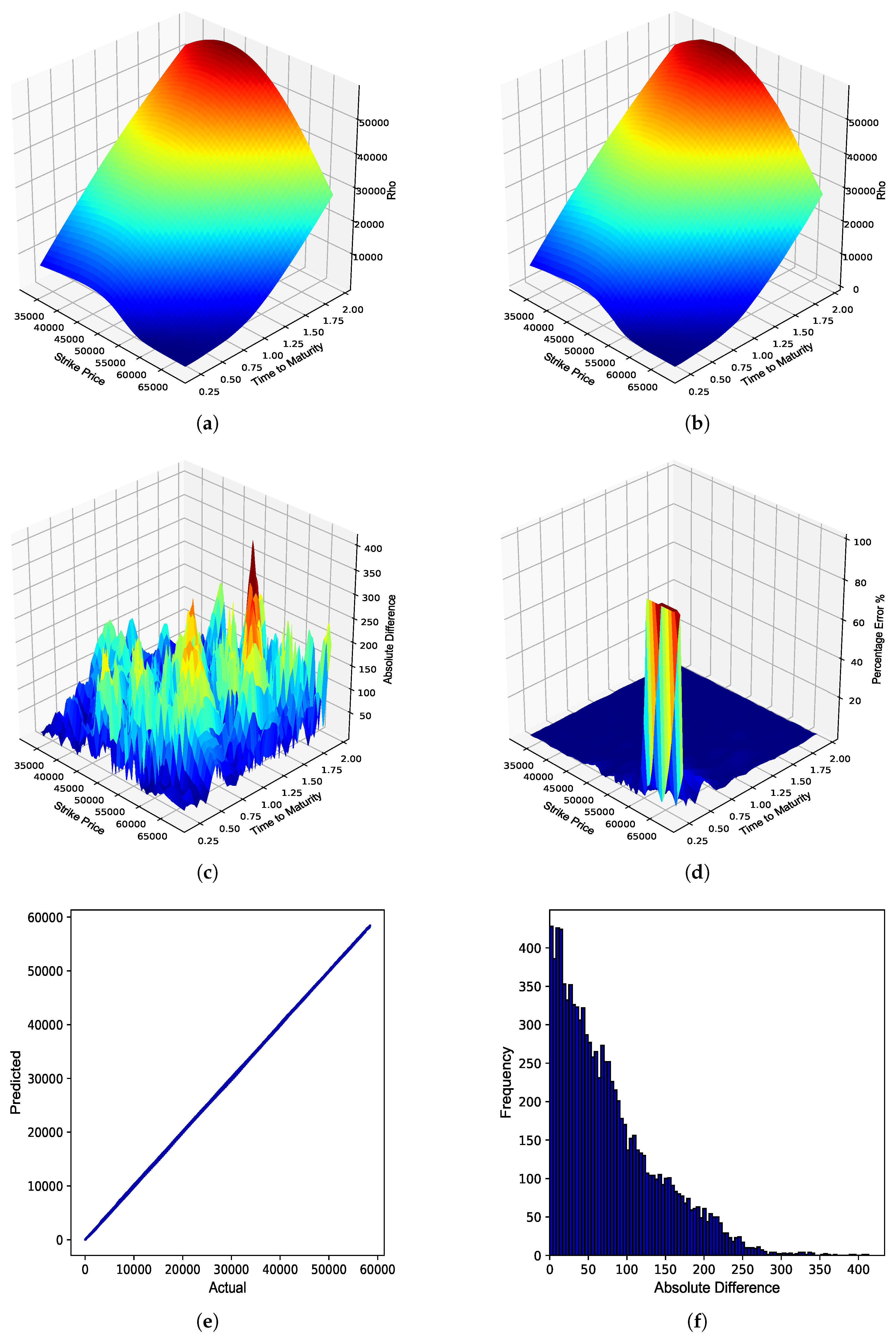
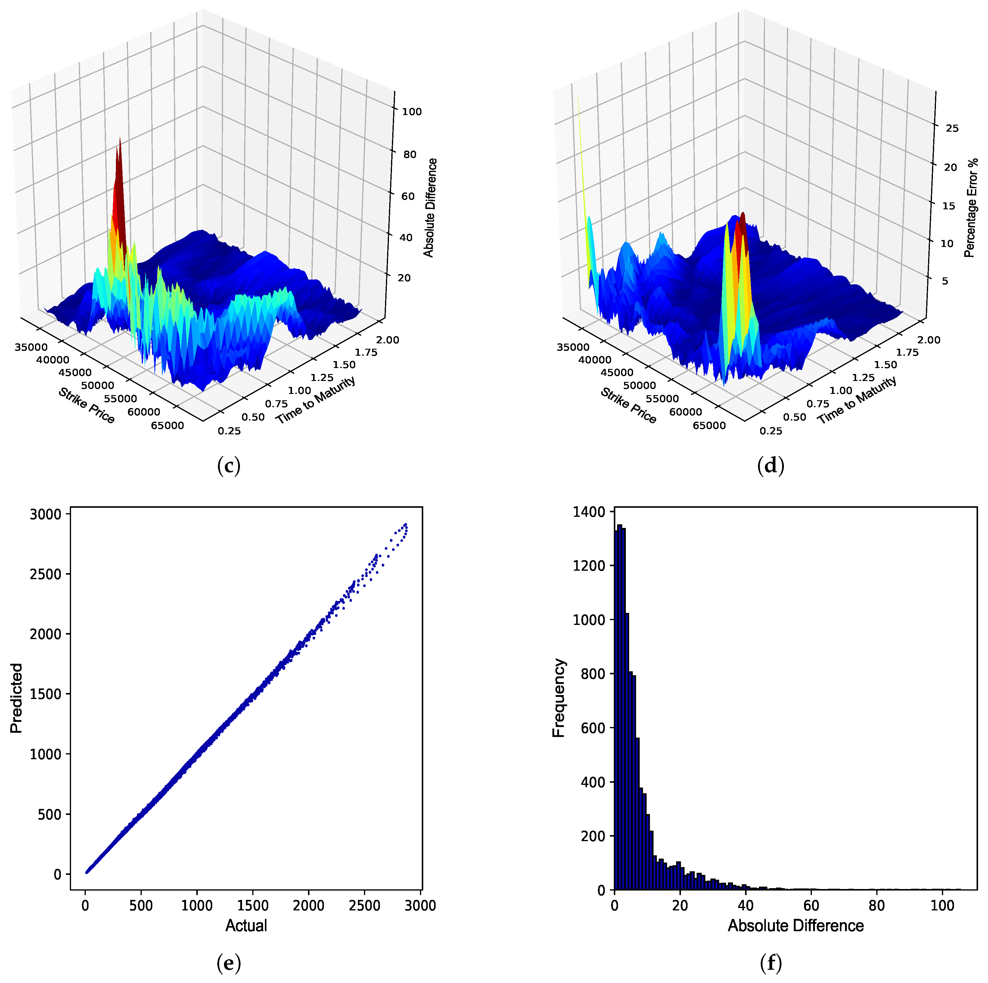
The optimized BS ANN Greeks were provided the test data set consisting of a constructed implied volatility surface as well as the other test set inputs, which were then used to generate JSE Top 40 European call option Greek surfaces. The sensitivity values generated by the BS ANN Greeks were then benchmarked against the values obtained using the explicit solutions to these option Greeks under the BS model. The performance of the BS ANN Greeks compared to the explicit solutions are detailed in
Table 4.
From
Table 4, it can be seen that the BS ANN Greeks were able to approximate the explicit solutions to the BS Greeks very well, as highlighted by the respective error metrics. A graphical overview of the overall performance of the respective BS ANN Greeks in approximating the option Greeks of JSE Top 40 European call options is provided in
Figure 2,
Figure 3,
Figure 4,
Figure 5 and
Figure 6.
In the next section, the out-of-sample performance of the optimized ANNs in approximating the option Greeks under the Piterbarg model is evaluated.
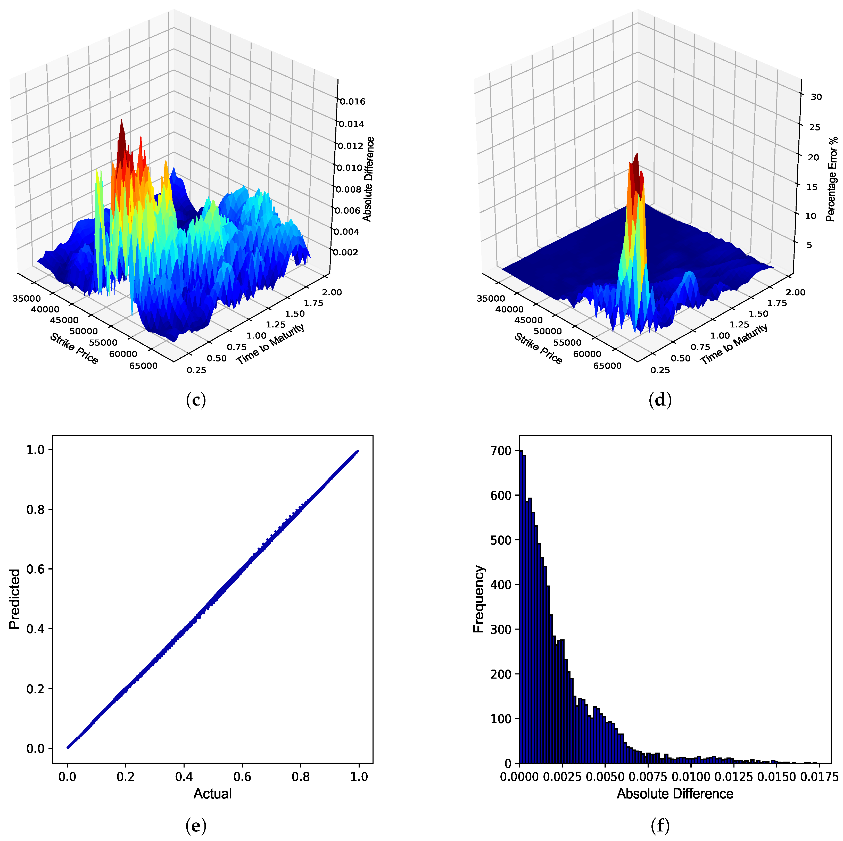
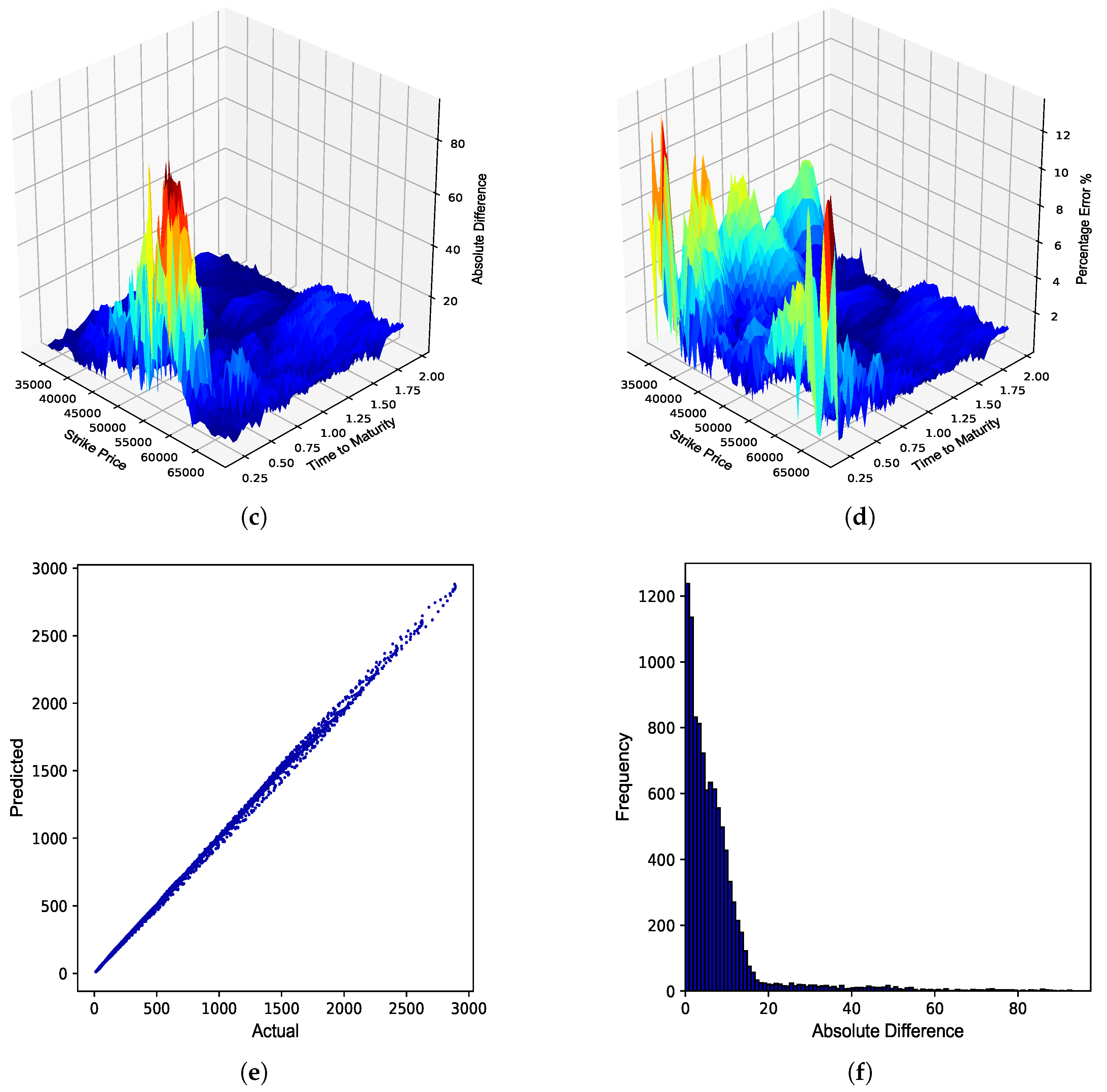
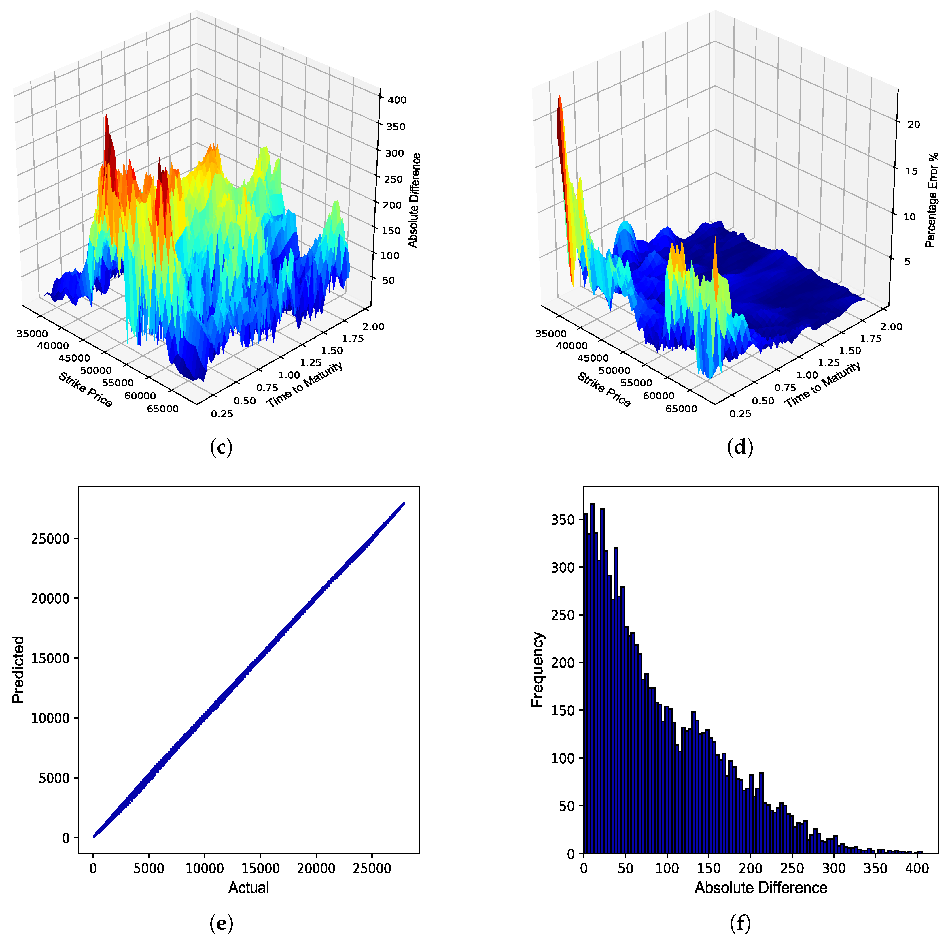
5.2. Numerical Results: Piterbarg Option Greeks
In this section, the performance of the optimized ZC and FC ANN Greeks is evaluated. The sensitivity values generated by the ZC and FC ANN Greeks were compared to the values obtained using the explicit solutions to the option Greeks under the Piterbarg model. The out-of-sample performance of the ZC and FC ANN Greeks compared to the explicit solutions under the Piterbarg model are detailed in
Table 5.
From
Table 5, similar conclusions as for the BS model in
Table 4 can be made, therefore highlighting that ANNs can also approximate the option Greeks in a multi-curve framework, such as the Piterbarg model, with a high degree of accuracy. The out-of-sample performance of the ZC and FC ANN Greeks is graphically illustrated in
Figure 7,
Figure 8,
Figure 9,
Figure 10,
Figure 11,
Figure 12,
Figure 13,
Figure 14,
Figure 15 and
Figure 16 and the findings of this paper are concluded in the next section.
6. Conclusions
The purpose of this paper was to build upon the existing financial machine learning literature by extending the use of machine learning techniques, such as ANNs, to the approximation of option price sensitivities in a BS and multi-curve framework, such as the Piterbarg model, that incorporates the effects of collateral on the price of a financial derivative. It was found that ANNs are able to approximate the respective option price sensitivities under the BS and Piterbarg models with a high degree of accuracy in a real-world out-of-sample application to the South African market.
The conclusions drawn from this paper are consistent with the observations made by
Ratku and Neumann (
2022) as well as
Umeorah et al. (
2023), and indicate that machine learning techniques, such as ANNs, can be utilized as an alternative data-driven approach to approximate the first- and second-order option price sensitivities. The results further highlight that even in the absence of sufficient option price data, especially in illiquid markets, such as South Africa, it is still possible to optimize ANNs on artificial training data and obtain satisfactory out-of-sample performance in a real-world setting. This is especially promising given that the approach used in this paper to generate artificial training data was fairly standard.
Areas of further research include exploring feasible solutions to the lack of representative training data in illiquid markets. Given that machine learning techniques are data-driven, it is pivotal to address this fundamental issue before we see the adoption of complex real-world applications that will undoubtedly redefine how financial markets interact in future.
Author Contributions
Conceptualization, R.d.P.; methodology, R.d.P.; software, R.d.P.; validation, P.J.V.; formal analysis, R.d.P.; investigation, R.d.P.; resources, P.J.V.; data curation, R.d.P.; writing—original draft preparation, R.d.P.; writing—review and editing, P.J.V.; visualization, R.d.P. and P.J.V.; supervision, P.J.V.; project administration, P.J.V.; funding acquisition, Not Applicable. All authors have read and agreed to the published version of the manuscript.
Funding
This research received no external funding.
Data Availability Statement
Data sharing is not applicable to this article.
Acknowledgments
The authors wish to thank the editor and anonymous referees for their constructive recommendations that helped improve the quality of the manuscript considerably.
Conflicts of Interest
The authors declare no conflicts of interest.
References
- Black, Fischer, and Myron Scholes. 1973. The Pricing of Options and Corporate Liabilities. Journal of Political Economy 81: 637–54. [Google Scholar] [CrossRef]
- Buehler, Hans, Lukas Gonon, Josef Teichmann, and Ben Wood. 2019. Deep Hedging. Quantitative Finance 19: 1271–91. [Google Scholar] [CrossRef]
- Chollet, François. 2015. Keras. Available online: https://github.com/fchollet/keras (accessed on 21 November 2020).
- Cybenko, George. 1989. Approximation by Superstitions of a Sigmoidal Function. Mathematics of Control, Signals and Systems 2: 303–14. [Google Scholar] [CrossRef]
- Heston, Steven L. 1993. A Closed-Form Solution for Options with Stochastic Volatility with Applications to Bond and Currency Options. Review of Financial Studies 6: 327–43. [Google Scholar] [CrossRef]
- Hornik, Kurt, Maxwell Stinchcombe, and Halbert White. 1989. Multilayer FeedForward Networks are Universal Approximators. Neural Networks 2: 359–66. [Google Scholar] [CrossRef]
- Hull, John C. 2009. Options, Futures and Other Derivatives, 7th ed. Hoboken: Prentice Hall. [Google Scholar]
- Hunzinger, Chadd B., and Coenraad C. A. Labuschagne. 2015. Pricing a Collateralized Derivative Trade with a Funding Value Adjustment. Journal of Risk and Financial Management 8: 17–42. [Google Scholar] [CrossRef]
- Hutchinson, James M., Andrew W. Lo, and Tomaso Poggio. 1994. A Nonparametric Approach to Pricing and Hedging Derivative Securities via Learning Networks. The Journal of Finance 49: 851–89. [Google Scholar] [CrossRef]
- Labuschagne, Coenraad C. A., and Sven T. von Boetticher. 2017. The Greeks of the Piterbarg Option Pricing Framework. Topics in Economics, Business and Management 1: 1–5. [Google Scholar]
- Leoni, Peter. 2014. The Greeks and Hedging Explained, 1st ed. London: Palgrave Macmillan. [Google Scholar]
- Piterbarg, Vladimir. 2010. Funding Beyond Discounting: Collateral Agreements and Derivatives Pricing. Risk Magazine 23: 97–102. [Google Scholar]
- Ratku, Antal, and Dirk Neumann. 2022. Derivatives of Feed-Forward Neural Networks and their Application in Real-time Market Risk Management. OR Spectrum 44: 947–65. [Google Scholar] [CrossRef]
- Ruf, Johannes, and Weiguan Wang. 2020. Neural Networks for Option Pricing and Hedging: A Literature Review. Journal of Computational Finance 24: 1–46. [Google Scholar] [CrossRef]
- Umeorah, Nneka, Phillip Mashele, Onyecherelam Agbaeze, and Jules Clement Mba. 2023. Barrier Options and Greeks: Modeling with Neural Networks. Axioms 12: 384. [Google Scholar] [CrossRef]
- von Boetticher, Sven Thorsten. 2017. The Piterbarg Framework for Option Pricing. Doctoral thesis, University of Johannesburg, Johannesburg, South Africa. [Google Scholar]
Figure 1.
JSE Top 40 implied volatility surface.
Figure 1.
JSE Top 40 implied volatility surface.
Figure 2.
JSE Top 40 European call option Delta. (a) Delta surface: Black–Scholes; (b) Delta surface: ANN; (c) Absolute error; (d) Percentage error; (e) Actual vs. predicted; (f) Frequency of errors.
Figure 2.
JSE Top 40 European call option Delta. (a) Delta surface: Black–Scholes; (b) Delta surface: ANN; (c) Absolute error; (d) Percentage error; (e) Actual vs. predicted; (f) Frequency of errors.
Figure 3.
JSE Top 40 European call option Dollar Gamma. (a) Dollar Gamma surface: Black–Scholes; (b) Dollar Gamma surface: ANN; (c) Absolute error; (d) Percentage error; (e) Actual vs. predicted; (f) Frequency of errors.
Figure 3.
JSE Top 40 European call option Dollar Gamma. (a) Dollar Gamma surface: Black–Scholes; (b) Dollar Gamma surface: ANN; (c) Absolute error; (d) Percentage error; (e) Actual vs. predicted; (f) Frequency of errors.
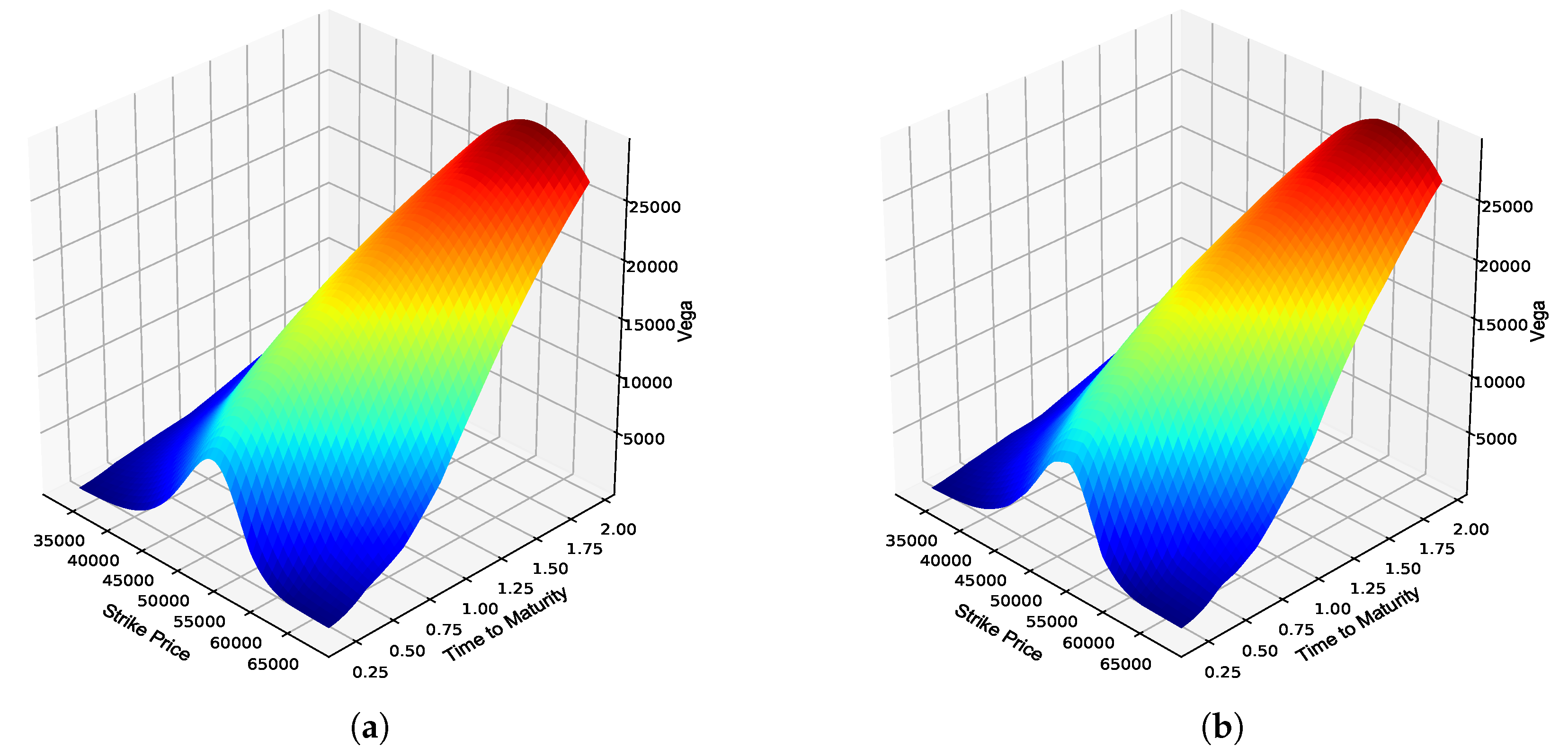
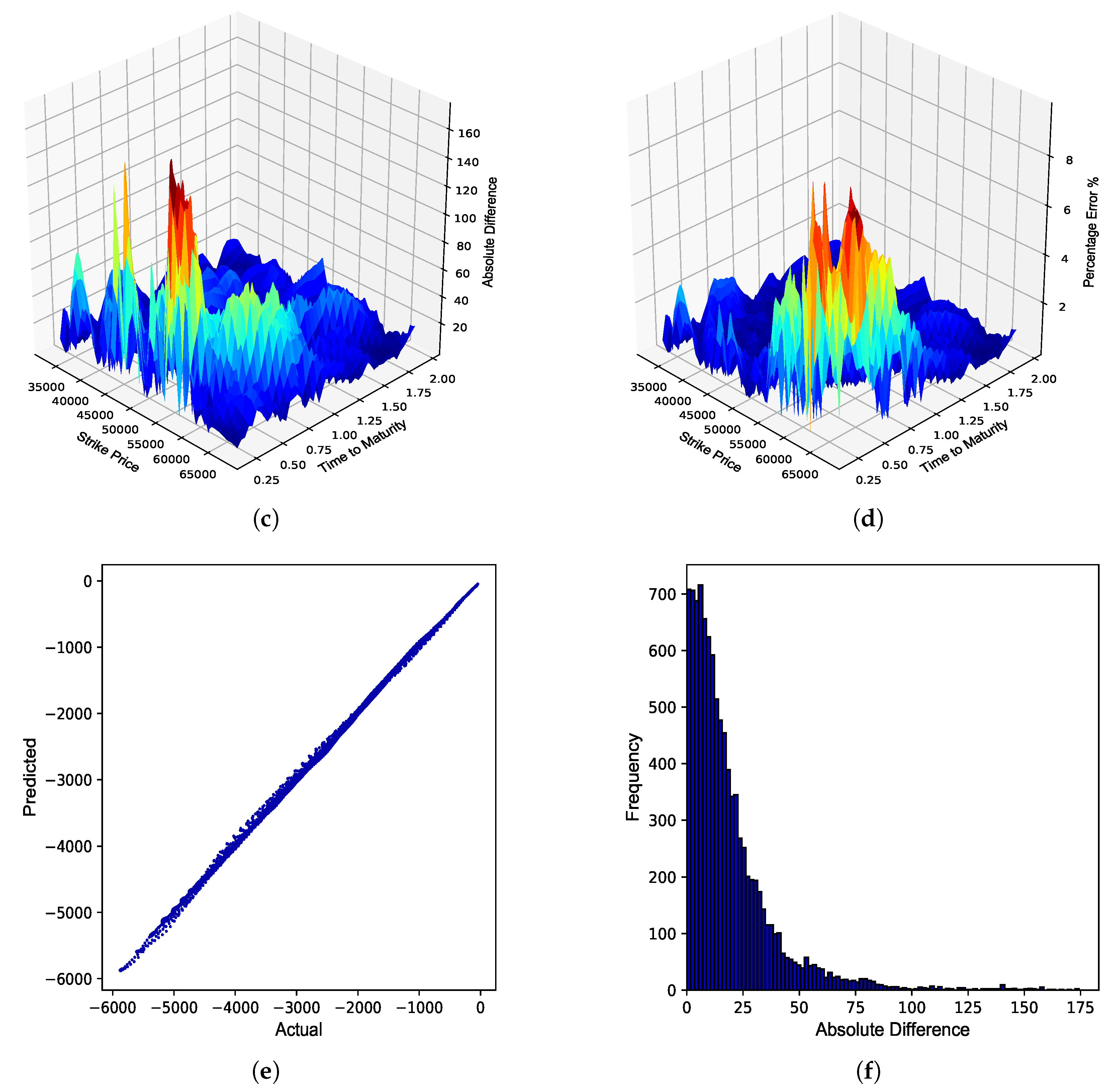
Figure 4.
JSE Top 40 European call option Vega. (a) Vega surface: Black–Scholes; (b) Vega surface: ANN; (c) Absolute error; (d) Percentage error; (e) Actual vs. predicted; (f) Frequency of errors.
Figure 4.
JSE Top 40 European call option Vega. (a) Vega surface: Black–Scholes; (b) Vega surface: ANN; (c) Absolute error; (d) Percentage error; (e) Actual vs. predicted; (f) Frequency of errors.
Figure 5.
JSE Top 40 European call option Theta. (a) Theta surface: Black–Scholes; (b) Theta surface: ANN; (c) Absolute error; (d) Percentage error; (e) Actual vs. predicted; (f) Frequency of errors.
Figure 5.
JSE Top 40 European call option Theta. (a) Theta surface: Black–Scholes; (b) Theta surface: ANN; (c) Absolute error; (d) Percentage error; (e) Actual vs. predicted; (f) Frequency of errors.
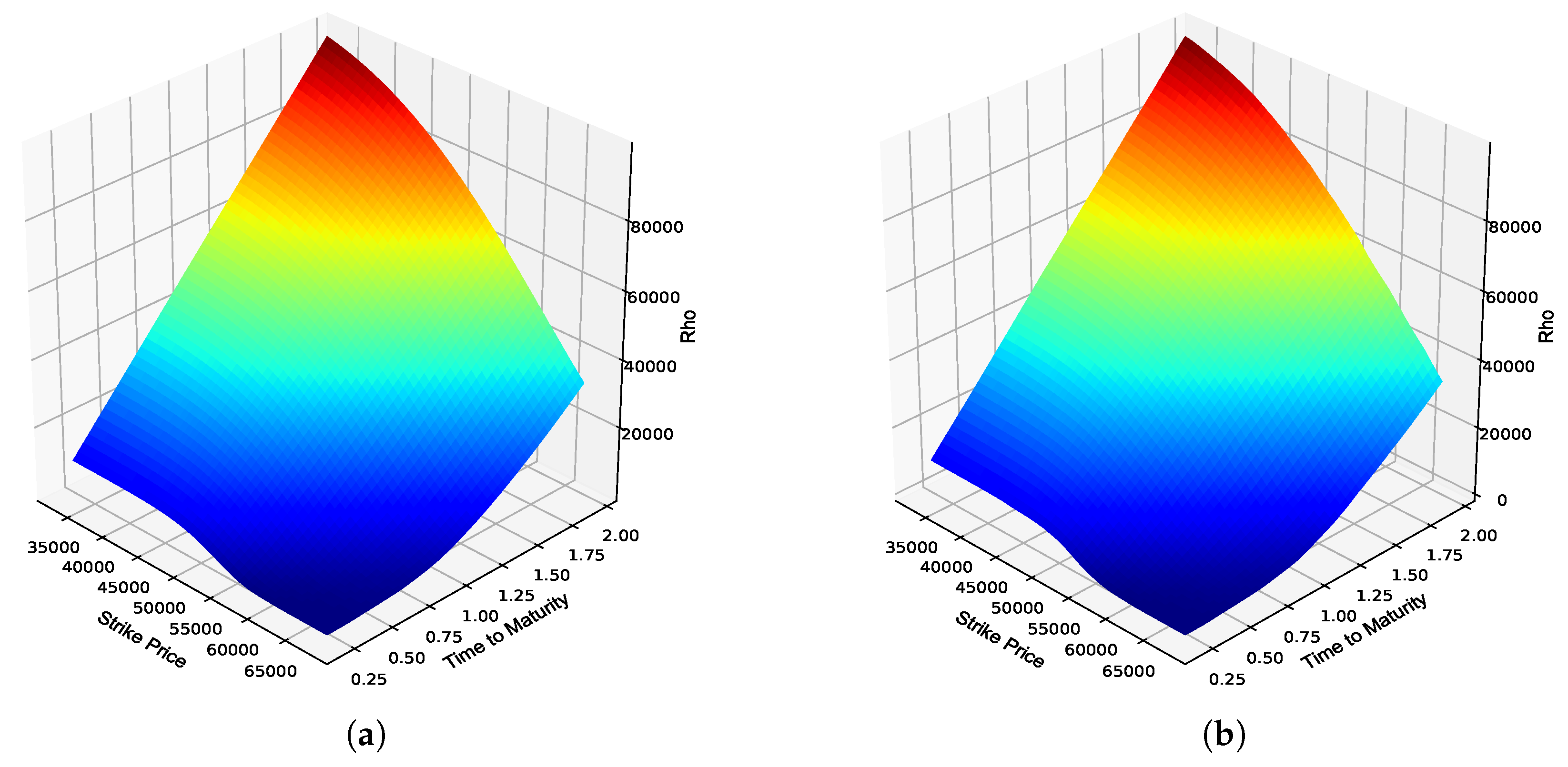
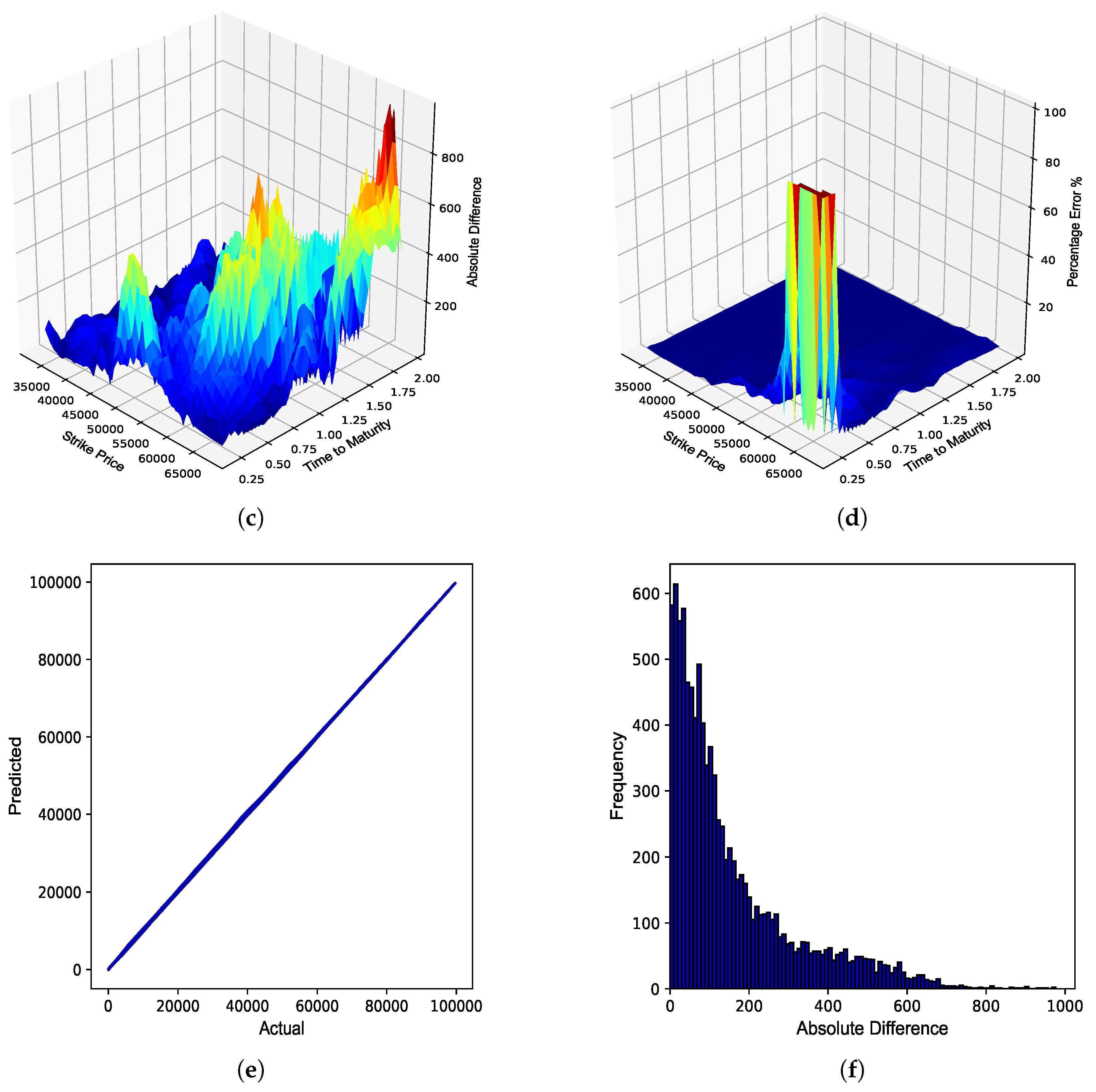
Figure 6.
JSE Top 40 European call option Rho. (a) Rho surface: Black–Scholes; (b) Rho surface: ANN; (c) Absolute error; (d) Percentage error; (e) Actual vs. predicted; (f) Frequency of errors.
Figure 6.
JSE Top 40 European call option Rho. (a) Rho surface: Black–Scholes; (b) Rho surface: ANN; (c) Absolute error; (d) Percentage error; (e) Actual vs. predicted; (f) Frequency of errors.
Figure 7.
JSE Top 40 zero collateral call option Delta. (a) Delta surface: Zero collateral; (b) Delta surface: ANN; (c) Absolute error; (d) Percentage error; (e) Actual vs. predicted; (f) Frequency of errors.
Figure 7.
JSE Top 40 zero collateral call option Delta. (a) Delta surface: Zero collateral; (b) Delta surface: ANN; (c) Absolute error; (d) Percentage error; (e) Actual vs. predicted; (f) Frequency of errors.
Figure 8.
JSE Top 40 fully collateralized call option Delta. (a) Delta surface: Fully collateralized; (b) Delta surface: ANN; (c) Absolute error; (d) Percentage error; (e) Actual vs. predicted; (f) Frequency of errors.
Figure 8.
JSE Top 40 fully collateralized call option Delta. (a) Delta surface: Fully collateralized; (b) Delta surface: ANN; (c) Absolute error; (d) Percentage error; (e) Actual vs. predicted; (f) Frequency of errors.
Figure 9.
JSE Top 40 zero collateral call option Dollar Gamma. (a) Dollar Gamma surface: Zero collateral; (b) Dollar Gamma surface: ANN; (c) Absolute error; (d) Percentage error; (e) Actual vs. predicted; (f) Frequency of errors.
Figure 9.
JSE Top 40 zero collateral call option Dollar Gamma. (a) Dollar Gamma surface: Zero collateral; (b) Dollar Gamma surface: ANN; (c) Absolute error; (d) Percentage error; (e) Actual vs. predicted; (f) Frequency of errors.
Figure 10.
JSE Top 40 fully collateralized call option Dollar Gamma. (a) Dollar Gamma surface: Fully collateralized; (b) Dollar Gamma surface: ANN; (c) Absolute error; (d) Percentage error; (e) Actual vs. predicted; (f) Frequency of errors.
Figure 10.
JSE Top 40 fully collateralized call option Dollar Gamma. (a) Dollar Gamma surface: Fully collateralized; (b) Dollar Gamma surface: ANN; (c) Absolute error; (d) Percentage error; (e) Actual vs. predicted; (f) Frequency of errors.
Figure 11.
JSE Top 40 zero collateral call option Vega. (a) Vega surface: Zero collateral; (b) Vega surface: ANN; (c) Absolute error; (d) Percentage error; (e) Actual vs. predicted; (f) Frequency of errors.
Figure 11.
JSE Top 40 zero collateral call option Vega. (a) Vega surface: Zero collateral; (b) Vega surface: ANN; (c) Absolute error; (d) Percentage error; (e) Actual vs. predicted; (f) Frequency of errors.
Figure 12.
JSE Top 40 fully collateralized call option Vega. (a) Vega surface: Fully collateralized; (b) Vega surface: ANN; (c) Absolute error; (d) Percentage error; (e) Actual vs. predicted; (f) Frequency of errors.
Figure 12.
JSE Top 40 fully collateralized call option Vega. (a) Vega surface: Fully collateralized; (b) Vega surface: ANN; (c) Absolute error; (d) Percentage error; (e) Actual vs. predicted; (f) Frequency of errors.
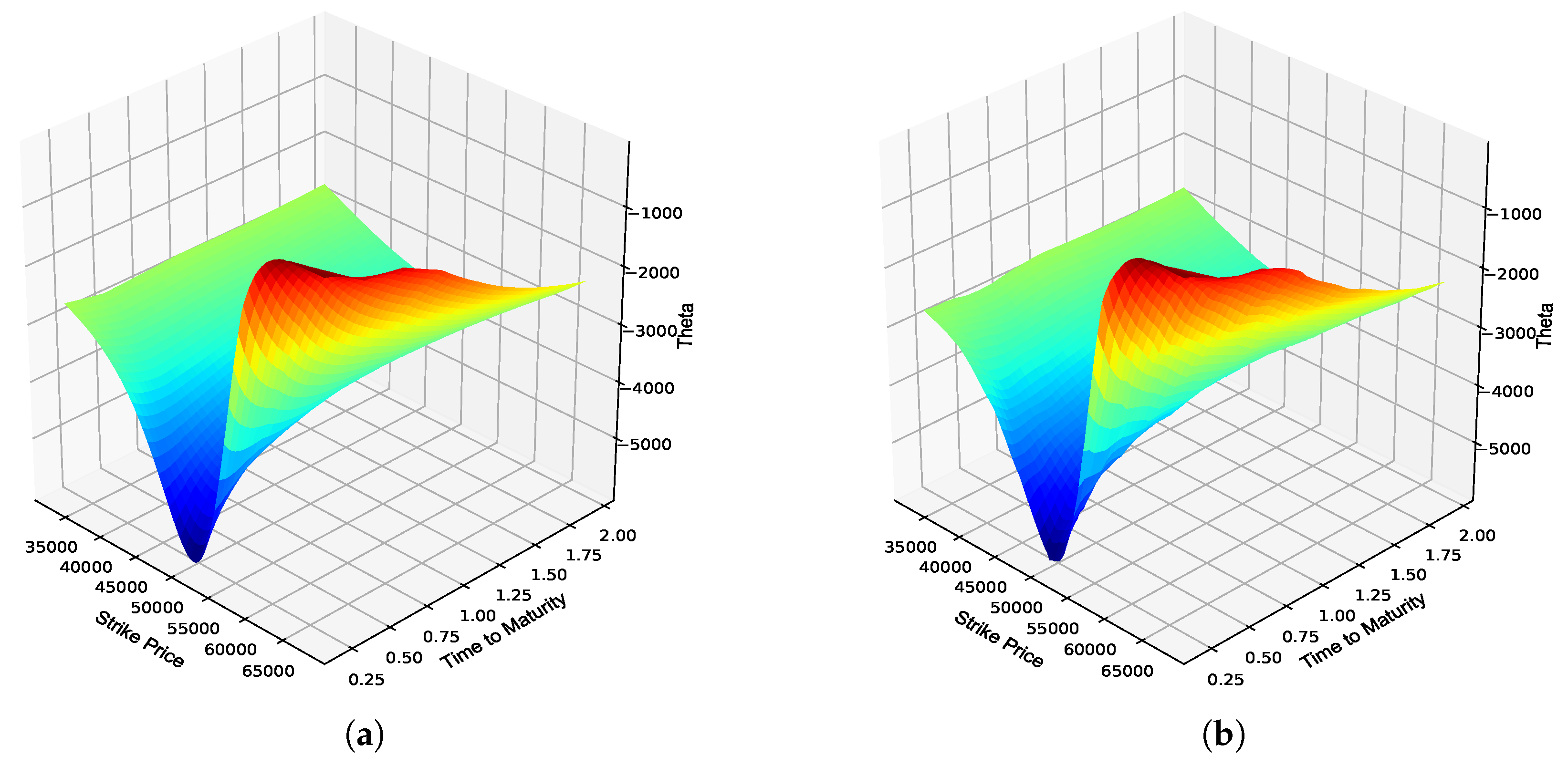
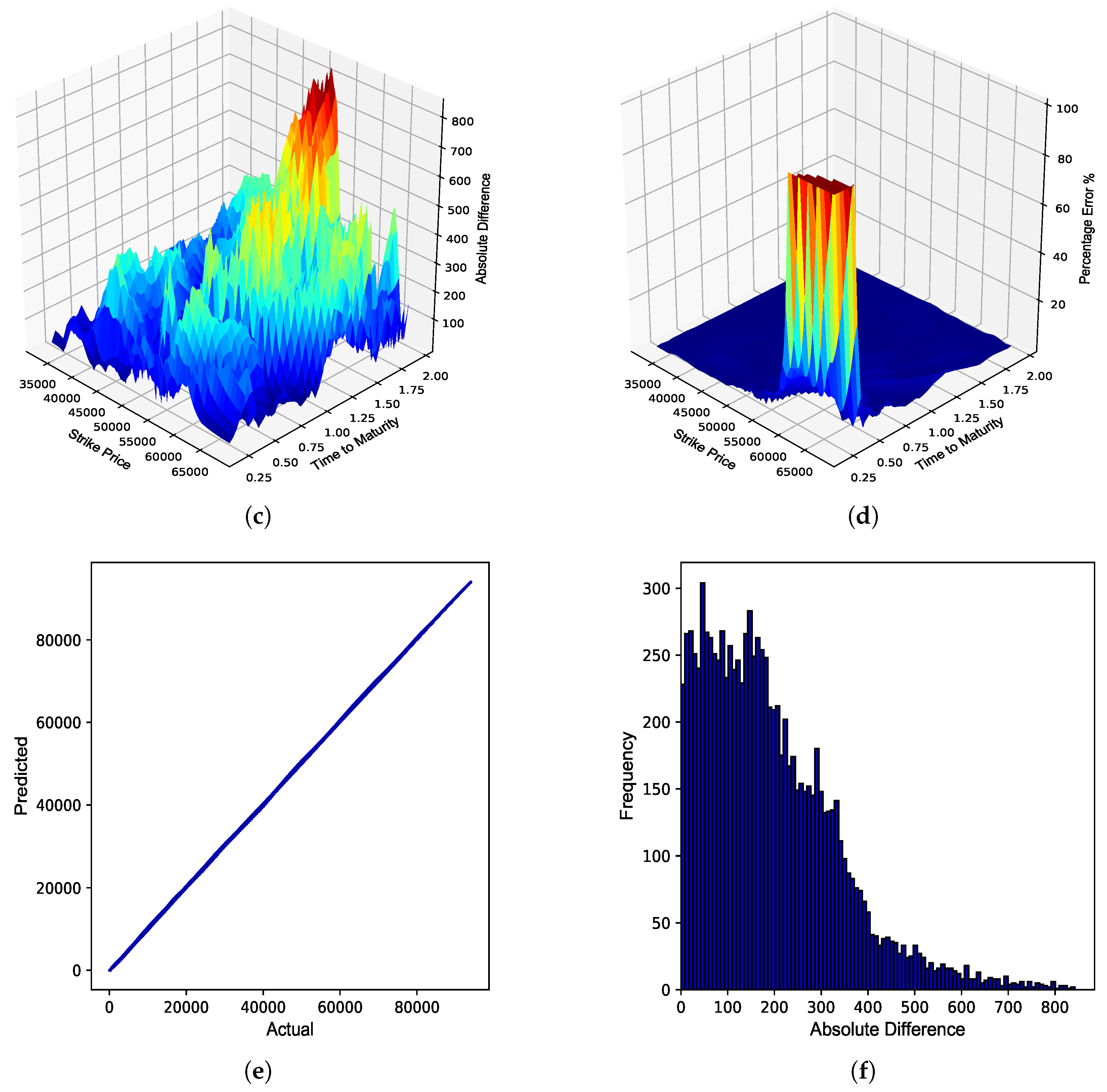
Figure 13.
JSE Top 40 zero collateral call option Theta. (a) Theta surface: Zero collateral; (b) Theta surface: ANN; (c) Absolute error; (d) Percentage error; (e) Actual vs. predicted; (f) Frequency of errors.
Figure 13.
JSE Top 40 zero collateral call option Theta. (a) Theta surface: Zero collateral; (b) Theta surface: ANN; (c) Absolute error; (d) Percentage error; (e) Actual vs. predicted; (f) Frequency of errors.
Figure 14.
JSE Top 40 fully collateralized call option Theta. (a) Theta surface: Fully collateralized; (b) Theta surface: ANN; (c) Absolute error; (d) Percentage error; (e) Actual vs. predicted; (f) Frequency of errors.
Figure 14.
JSE Top 40 fully collateralized call option Theta. (a) Theta surface: Fully collateralized; (b) Theta surface: ANN; (c) Absolute error; (d) Percentage error; (e) Actual vs. predicted; (f) Frequency of errors.
Figure 15.
JSE Top 40 zero collateral call option Rho. (a) Rho surface: Zero collateral; (b) Rho surface: ANN; (c) Absolute error; (d) Percentage error; (e) Actual vs. predicted; (f) Frequency of errors.
Figure 15.
JSE Top 40 zero collateral call option Rho. (a) Rho surface: Zero collateral; (b) Rho surface: ANN; (c) Absolute error; (d) Percentage error; (e) Actual vs. predicted; (f) Frequency of errors.
Figure 16.
JSE Top 40 fully collateralized call option Rho. (a) Rho surface: Fully collateralized; (b) Rho surface: ANN; (c) Absolute error; (d) Percentage error; (e) Actual vs. predicted; (f) Frequency of errors.
Figure 16.
JSE Top 40 fully collateralized call option Rho. (a) Rho surface: Fully collateralized; (b) Rho surface: ANN; (c) Absolute error; (d) Percentage error; (e) Actual vs. predicted; (f) Frequency of errors.
Table 1.
General ANN Greek configuration.
Table 1.
General ANN Greek configuration.
| Parameter | Delta | Dollar Gamma | Vega | Theta | Rho |
|---|
| Hidden layers | 4 | 4 | 4 | 4 | 4 |
| Neurons per hidden layer | 256 | 256 | 256 | 256 | 256 |
| Neurons in output layer | 1 | 1 | 1 | 1 | 1 |
| Hidden activation function | ReLU | ReLU | ReLU | ReLU | ReLU |
| Output activation function | Sigmoid 1 | Softplus | Softplus | Linear | Softplus |
| Optimiser | Adam | Adam | Adam | Adam | Adam |
| Batch size | 64 | 64 | 64 | 64 | 64 |
| Epochs | 50 | 50 | 50 | 50 | 50 |
| Loss function | MAE | MAE | MAE | MAE | MAE |
| Early stopping | Yes | Yes | Yes | Yes | Yes |
Table 2.
Black–Scholes model input parameter ranges.
Table 2.
Black–Scholes model input parameter ranges.
| Parameter | Range |
|---|
| Moneyness () | 0.25–2.00 |
| Time to maturity () | 7/365–3.50 |
| Risk-free rate (r) | 3.00–35.00% |
| Implied volatility () | 2.00–80.00% |
Table 3.
Piterbarg model input parameter ranges.
Table 3.
Piterbarg model input parameter ranges.
| Parameter | Range |
|---|
| Moneyness () | 0.25–2.00 |
| Time to maturity () | 7/365–3.50 |
| Repurchase agreement rate () | 3.00–35.00% |
| Collateral rate () | 60.00–80.00% of |
| Funding rate () | 120.00–140.00% of |
| Implied volatility () | 2.00–80.00% |
Table 4.
BS ANN Greek error metrics.
Table 4.
BS ANN Greek error metrics.
| Greek | MAE | MAPE | |
|---|
| Delta | 0.001960 | 0.988138% | 0.999911 |
| Dollar Gamma | 9.410143 | 2.312544% | 0.999331 |
| Vega | 74.368062 | 1.083190% | 0.999863 |
| Theta | 23.146617 | 0.978941% | 0.999080 |
| Rho | 76.742017 | 1.504959% | 0.999962 |
Table 5.
Piterbarg ANN Greek error metrics.
Table 5.
Piterbarg ANN Greek error metrics.
| Greek | MAE | MAPE | |
|---|
| ZC Delta | 0.002313 | 0.886302% | 0.999876 |
| FC Delta | 0.002467 | 0.901067% | 0.999853 |
| ZC Dollar Gamma | 6.993475 | 1.369866% | 0.999402 |
| FC Dollar Gamma | 7.523029 | 1.525594% | 0.999246 |
| ZC Vega | 91.628587 | 1.390869% | 0.999767 |
| FC Vega | 97.614717 | 1.537854% | 0.999720 |
| ZC Theta | 18.890212 | 0.945713% | 0.999191 |
| FC Theta | 24.170855 | 0.976136% | 0.998857 |
| ZC Rho | 191.633702 | 3.312146% | 0.999901 |
| FC Rho | 157.464666 | 2.528751% | 0.999922 |
| Disclaimer/Publisher’s Note: The statements, opinions and data contained in all publications are solely those of the individual author(s) and contributor(s) and not of MDPI and/or the editor(s). MDPI and/or the editor(s) disclaim responsibility for any injury to people or property resulting from any ideas, methods, instructions or products referred to in the content. |
© 2024 by the authors. Licensee MDPI, Basel, Switzerland. This article is an open access article distributed under the terms and conditions of the Creative Commons Attribution (CC BY) license (https://creativecommons.org/licenses/by/4.0/).


