Article

The Extent and Efficiency of Credit Reallocation During Economic Downturns

1
Faculty of Economics, Kyoto Sangyo University, Motoyama Kamigamo Kita-ku, Kyoto 603-8047, Japan
2
Institute of Economic Research, Hitotsubashi University, 2-1 Naka-Kunitachi, Tokyo 186-8603, Japan
3
Research Institute of Economy, Trade and Industry, 1-3-1 Kasumigaseki, Chiyoda-ku, Tokyo 100-8901, Japan
*
Author to whom correspondence should be addressed.
J. Risk Financial Manag. 2024, 17(12), 574; https://doi.org/10.3390/jrfm17120574
Submission received: 20 October 2024 / Revised: 29 November 2024 / Accepted: 9 December 2024 / Published: 19 December 2024
(This article belongs to the Special Issue Financial Markets and Institutions)

Abstract

The theoretical literature on credit reallocation has yielded conflicting predictions on both the extent and the efficiency of reallocations during economic downturns. We borrowed the methodology of measuring job reallocation to measure credit reallocation and examine which predictions are consistent with the data. We reported the following findings: (1) the extent of credit reallocation is smaller in recessions than in expansions, which is attributable to the decreasing extent of credit creation; (2) this tendency was more pronounced during the Lost Decade of the 1990s; (3) credit reallocation generally is efficiency-enhancing, but at a lower rate in recessions and turns to efficiency-reducing during the Lost Decade, possibly due to financial assistance by banks to large but low-quality firms (e.g., through zombie lending). These findings indicate that the inefficient credit reallocation during the Lost Decade was characterized by efficiency-reducing reallocation to large firms.
JEL Classification:
E44; E51; G30

1. Introduction

The interfirm allocations of physical and financial inputs for production, such as labor, capital, and external finance, are as important for the performance and efficiency of an economy as the sheer amounts of these inputs. These allocations have motivated many economists to construct aggregate measures for input reallocation and to examine the link between the extent of input reallocation and the business cycle. They first focused on the reallocations of jobs and physical capital across firms (Davis and Haltiwanger 1992; Davis et al. 1996; Ramey and Shapiro 1998; Eisfeldt and Rampini 2006). Economists then turned to the reallocation of external financial resources, led by the seminal study by Herrera et al. (2011) who examined the extent and cyclicality of the credit reallocations of large firms in the United States.1 That study was followed by Herrera et al.’s (2014) study on the impact of credit reallocation on US economic growth and Hyun and Minetti’s (2019) study on credit reallocation in Korea before and after the country’s financial crisis in 1997.2
Turning from empirical to theoretical research on the reallocation of resources, studies have arrived at conflicting predictions in several respects, such as the extent, cyclicality, and efficiency of resource reallocation. For example, Caballero and Hammour (1994) and Den Haan et al. (2003) suggest that the extent of reallocation increases when the economy is in a downturn, while Caballero and Hammour (2005) and Chamley and Rochon (2011) argue the opposite and predict that the extent of reallocation is smaller in a recession. Another respect in which studies yield conflicting predictions is with regard to the degree to which reallocation is efficiency-enhancing at different stages of the business cycle. Becsi et al. (2005) argue that efficiency-enhancing reallocation is more pronounced during economic downturns, while Barlevy (2003) predicts that reallocation is actually efficiency-reducing in recessions.3 Yet, despite this lack of consensus, empirical research on the reallocation of resources—including research on the reallocation of credit—has tended to focus on discovering solid statistical regularities rather than on examining which of the conflicting theoretical views is supported by the data.
Against this background, the aim of this study is to empirically test hypotheses on the extent and efficiency of credit reallocation during economic downturns in Japan. To test these hypotheses, we construct measures of credit reallocation for firms of all sizes in Japan covering the period from 1980 to 2014 and investigate its extent, especially during periods of economic contraction. We then examine if it is efficiency-enhancing in that credit generally flows from low-productivity to high-productivity firms and if the extent of efficiency-enhancing reallocation in recessionary times differs from normal times. We employ quarterly financial statements data for both large firms and small and medium-sized enterprises (SMEs) spanning our sample period. Japan is an especially interesting laboratory for researchers to empirically test these hypotheses on credit reallocation. As shown in Figure 1, it is a country where debt financing plays a much more important role than in the United States, and an academic assessment of credit reallocation may hold important lessons for other countries in which debt financing plays a relevant role. However, to date, there are no studies on credit reallocation in Japan.
Our analysis yields the following three major findings. First, the extent of credit reallocation is smaller in recessions than in expansions, which is attributable to the decreasing extent of credit creation. Second, this tendency was more pronounced during the Lost Decade of the 1990s. Third, credit reallocation generally is efficiency-enhancing, but it becomes efficiency-reducing during the Lost Decade, possibly due to financial assistance by banks to large but low-quality firms. These findings together indicate that the inefficient credit reallocation during the Lost Decade was characterized by efficiency-reducing reallocation for large firms.
Our study contributes to the literature in three respects. First, it is the first to construct credit reallocation measures for both large firms and SMEs and to examine credit reallocation across all firms of a country. Our measures therefore allow us to compare the extent of, and fluctuations in, the credit reallocations across firms of different sizes.
Second, we employ total factor productivity (TFP) at the firm level to examine the relationship between credit reallocation and productivity to see whether reallocation is efficiency-enhancing or efficiency-reducing, that is, whether credit flows from low-productivity to high-productivity firms or the other way around. Further, we also examine whether the efficiency-enhancing nature of reallocation is more pronounced or dampened during economic downturns, and if so, how.
Third, we shed new light on the efficiency of the Japanese loan market from a long-term perspective. While the Lost Decade of the 1990s, which saw the emergence of a severe financial crisis, has spawned a substantial body of empirical and theoretical literature on how the crisis unfolded and affected the efficiency of the credit market (e.g., Peek and Rosengren 2005; Caballero et al. 2008; Chamley and Rochon 2011; and Sakai et al. 2010), in our study, we examine a much longer time horizon. Specifically, we examine the efficiency of the market over more than three decades, while most preceding studies only cover the 1990s and the early 2000s, including the period of the Japanese financial crisis at the end of the 1990s. Therefore, our analysis is able to provide a broader perspective of the efficiency of the financial market during economic downturns and offer important policy implications for how governments should respond to the inefficiencies in the market. Further, there have been a number of studies that examine credit market efficiency in countries other than Japan, especially after the 2007–2008 global financial crisis (e.g., Iyer et al. 2014; Sette and Gobbi 2015; Beck et al. 2018; and Banerjee and Hofmann 2018). Since these studies adopt the approaches used by Peek and Rosengren (2005) and Caballero et al. (2008), our study provides results that allow comparisons with these studies.
The study proceeds as follows: In Section 2, we review the literature and pose our empirical hypotheses. In Section 3, we describe our data and several key variables, while we detail our empirical approach in Section 4. Section 5 and Section 6 present the results; in Section 5, we discuss the extent of credit reallocation during economic downturns, and we focus on the efficiency of reallocation in Section 6. Section 7 concludes.

2. Literature Review and Hypotheses

2.1. Size of Reallocation During Economic Downturns

Research on the reallocation of resources for production, such as labor, capital, and credit, focuses on two distinct but interrelated aspects: the creation of new production arrangements, and the destruction of obsolete arrangements. One of the primary objectives of studies on resource reallocation is to examine what happens when there is a negative shock to the economy; that is, how the creation and destruction of production arrangements are affected during an economic downturn.
One of the earliest theoretical studies on resource reallocation is that by Caballero and Hammour (1994) who examine the responses of the creation and destruction of production arrangements to cyclical variations in demand. Assuming nonlinear adjustment costs, they argue that the structure of creation costs gives industries a motive for smoothing the creation process and accommodating fluctuations in demand primarily through the destruction of production units. They therefore predict that reallocation will be more sizeable during economic downturns than during booms and that most of this reallocation is driven by the increase in the destruction of production units. Den Haan et al. (2003) present a dynamic equilibrium model of the credit market with a focus on the role of matches formed by lenders and entrepreneurs. Their model shows that the extent to which those relationships between lenders and entrepreneurs break up is larger during recessions, resulting in greater credit reallocation. On the other hand, credit creation responds only slowly and makes only a relatively minor contribution to the change in credit reallocation.
These studies point to the possibility that, on the one hand, the extent of destruction of jobs, capital, and credit increases in recessions, leading to an increase in resource reallocation. On the other hand, the extent to which these productive resources are created decreases in recessions or remains stable at best. Summarizing the above discussion and focusing on the reallocation of credit, we posit the following hypothesis:
Hypothesis 1 (H1):
The extent of credit reallocation becomes larger during economic downturns, driven by an increase in the extent of credit destruction.
The empirical evidence for an increase in credit destruction during recessions is provided by Herrera et al. (2011) for the US and Hyun and Minetti (2019) for Korea. However, in Japan, where bank–firm relationships last much longer than in other countries, destruction of credit during economic downturns might not be as severe as elsewhere.4
We therefore also consider an alternative to Hypothesis 1 based on the theoretical study by Chamley and Rochon (2011) who predict that bank–firm relationships continue to last during downturns. Specifically, focusing on the reallocation of credit, Chamley and Rochon (2011) employ a search and matching model of the credit market in which banks choose between short-term and long-term loans. In recessions, when the profitability of new loans decreases and verification costs for projects financed through long-term loans increases, banks choose to roll over loans. Such behavior of banks will result in a lower level of credit destruction and creation and a smaller extent of credit reallocation. This argument can be summarized in the following hypothesis:
Hypothesis 1′ (H1′):
Alternatively, the extent of credit reallocation becomes smaller during economic downturns. The extent of both credit destruction and creation remains stable or decreases.

2.2. Existence and Extent of Efficiency-Enhancing Resource Reallocation

Another important objective of the studies on resource reallocation is to examine if it is efficiency-enhancing; that is, if resources flow from the least productive to the most productive units. Many of the studies referred to in the previous subsection, including the study by Caballero and Hammour (1994), assume that reallocation is efficiency-enhancing. In their setups, only the most efficient production units participate in the production process. If the number of production units is insufficient, other production units enter the market based on a strict productivity ranking. By the same logic, if the number is excessive, the least efficient units go out of business. Applying their assumptions to the reallocation of credit, these studies yield the following hypothesis:
Hypothesis 2 (H2):
Credit reallocation is efficiency-enhancing; that is, high-productivity firms are more likely to receive more credit and less likely to receive less credit than low-productivity firms.
The extent to which reallocation is efficiency-enhancing may change during economic downturns. Some studies argue that the extent may increase during a downturn in that a larger amount of resources flows from low-quality to high-quality firms during a recession than normal times. Becsi et al. (2005) develop a search and matching model for the provision of credit that incorporates heterogeneity in the quality of entrepreneurs (high quality and low quality). A negative shock leading to a recession has a disproportionately adverse impact on low-quality firms, leading to a breakup of existing matches these firms have with lenders. Thus, there will be a wider gap in credit availability between low-productivity and high-productivity firms during a downturn. The above argument yields the following hypothesis:
Hypothesis 3 (H3):
The extent of efficiency-enhancing credit reallocation is more pronounced during economic downturns.
In contrast, other studies yield the opposite prediction of Hypothesis 3 and suggest that reallocation is less efficiency-enhancing or even efficiency-reducing during a downturn. In a state of less efficiency-enhancing reallocation, a larger number of unprofitable and nonviable production units remain in the market than in normal times, but exit and survival of production units is still based on the order of their productivity. In a state of efficiency-reducing reallocation, the productivity order for reallocation is reversed; that is, low-productivity firms are more likely to receive more credit than high-productivity firms.
Such predictions are based on two lines of reasoning. The first focuses on more severe frictions in the market for resources used for production. Caballero and Hammour (2005) incorporate frictions in the labor and/or credit markets into their model to show that resource reallocation may be either less efficiency-enhancing or efficiency-reducing. They call these situations “sclerosis” and “scrambling”, respectively. A possible reason for such scrambling could be that, as highlighted by Barlevy (2003), the presence of credit market frictions may direct resources from more efficient to less efficient uses. Since, in practice, small firms are more likely to be financially constrained than large firms, we expect that this line of reasoning applies more to firms that are small in size.5
The second line of reasoning focuses on lenders’ incentives and argues that lenders provide financial assistance to unproductive and nonviable firms in recessions and try to extend zombie lending to these firms. Such behavior leads to either less efficiency-enhancing or to efficiency-reducing credit reallocation during economic downturns. Dewatripont and Maskin (1995) and Berglöf and Roland (1997), for example, make this point couching their analyses in terms of a dynamic commitment problem for lenders. In the presence of sunk costs for prior investment, lenders find it profitable ex post to refinance firms with ex ante unprofitable projects.6 Note that the above argument is more likely to hold for large loans if transaction costs for refinancing are fixed and minor relative to the benefits from lending to zombie firms. Fukuda et al. (2007) present other reasons for zombie lending than the problem of dynamic commitment, such as the difficulty of coordinating lenders and the political costs of liquidating too-big-to-fail firms. These issues are more serious in the case of loans to large firms than to small firms. Further, several empirical studies show evidence for the zombie lending to large listed firms (Peek and Rosengren 2005; Hoshi and Kashyap 2004), while others argue that banks extend these loans to small businesses only occasionally (Fukuda et al. 2007).7 The arguments presented in the above discussion are summarized in the following alternative hypothesis on the efficiency of credit reallocation in a downturn:
Hypothesis 3′ (H3′):
Alternatively, credit reallocation becomes less efficiency-enhancing and may even become efficiency-reducing during a downturn. If financial constraints play a role, the tendency of reallocation being less efficiency-enhancing will be more pronounced for small firms, while it will be more pronounced for large firms if the dynamic commitment or the too-big-to-fail issue matters for lenders.
In the sections that follow, we examine which of these hypotheses are consistent with the data. We achieve this by using data on firm financing in Japan for more than three decades from 1980 to 2014.

3. Data

In this section, we describe the data set and major variables we use for our analysis. Specifically, we present details of our data sources and then explain how we measure credit reallocation.

3.1. Data Sources

The main data source for our analysis is the Quarterly Financial Statements Statistics of Corporations by Industry (QFSSC) published by the Ministry of Finance of the Japanese government. An additional data source is the Japan Industrial Productivity (JIP) database for industry-level deflators and average working hours that we use to construct our firm-level productivity variable (TFP).8 The QFSSC is a survey of business corporations with paid-in capital of at least JPY 10 million headquartered in Japan. The QFSSC contains information such as firms’ balance sheets, employment, industry, and geographic location., and it covers all industries in both the manufacturing and the non-manufacturing sectors, although we exclude the financial and insurance industries from the analysis.9 The QFSSC comprises two parts: a part that targets all large corporations, and a part that consists of a sample of smaller firms. For the latter part, firms are randomly chosen and given questionnaires for four to eight quarters (one to two years). Throughout the analysis, we set the paid-in capital threshold value to distinguish between large firms and SMEs to JPY 100 million, following the criterion set by the Ministry of Finance. Details about what firms are chosen for the first part and how smaller firms are sampled are provided in Appendix A.

3.2. Construction of Credit Reallocation Measures

To measure the extent of credit reallocation, we employ the approach of Davis and Haltiwanger (1992) and Herrera et al. (2011), using balance sheet information from the QFSSC. c f t represents the average of firm f’s debt at time t − 1 and t. For the set of firms F s t belonging to sector s, we define C s t as the sum of c f t . We define the time t debt growth rate of a firm, g f t , as the first difference in its debt between time t − 1 and t divided by c f t . This measure takes a value from −2 to +2.10
Further, we introduce two measures, credit creation and credit destruction. Credit creation is the sum of the debt growth rates of firms with increasing debt. For the set of firms F s t , we calculate credit creation at time t ( P O S s t ) as the weighted sum of the debt growth rates of firms with increasing debt. Similarly, credit destruction is the sum of the debt growth rates of firms with declining debt. Specifically, we calculate credit destruction at time t ( N E G s t ) as the weighted sum of the absolute values of the debt growth rates of firms with decreasing debt.
Using c f t C s t as weights, we define the measures for credit creation and destruction as follows:
P O S s t = f F s t g f t > 0 c f t C s t g f t
N E G s t = f F s t g f t < 0 c f t C s t g f t
We define credit reallocation at time t ( S U M s t ) as the sum of credit creation and credit destruction, which represents the magnitude of the reshuffling of credit among firms.
S U M s t = P O S s t + N E G s t
In addition, we also define the net change in credit at time t ( N E T s t ) that is the difference between credit creation ( P O S s t ) and credit destruction ( N E G s t ):
N E T s t = P O S s t N E G s t
We define another measure of credit reallocation, which we call “excess credit reallocation” ( E X C s t ), as the difference between credit reallocation ( S U M s t ) and the absolute value of net credit growth ( N E T s t ), which is shown below:
E X C s t = S U M s t N E T s t .
A net increase in credit can be achieved through positive credit creation and no credit destruction. Alternatively, a net credit decrease can be achieved through positive credit destruction and no credit creation. Hence, E X C s t measures credit reallocation in excess of the minimum required for net credit changes.
To construct our measures of credit reallocation, we could use a number of different variables, namely, interest-bearing debt, loans from financial institutions, short-term loans from financial institutions, long-term loans from financial institutions, and corporate bonds. The variable that we mainly focus on in our analysis is interest-bearing debt, since it is the most comprehensive indicator of firms’ debt financing, as it includes the other four variables. We also use the loans from financial institutions in some analyses as some parts of the hypotheses are constructed based on theories on the behavior of financial institutions.
Three additional comments regarding the details and the validity of the credit reallocation measures we construct are in order. First, we use firm-level information rather than contract-level or project-level information for the credit reallocation measures. Firm-level information is suitable if a bank extends loans to a firm based on the firm’s creditworthiness, while contract- or project-level information is suitable if a bank provides project financing based on the prospective profitability of an individual project implemented by the firm. Since a large part of our sample consists of small firms that are too small to implement multiple projects simultaneously, we think that it is more appropriate to use firm-level information.
Second, we focus on the reallocation among surviving firms rather than including entering and exiting firms in our main analysis. This is due to the lack of information on firms’ entries and exits in the QFSSC. More specifically, we limit our calculation of g f t to firms for which observations at both ends of the interval between time t − 1 and t are available and exclude new entering and exiting firms for which no data are available at the beginning or end of the time interval. Excluding these entering and exiting firms from the sample results in a downward bias in our reallocation measures: P O S s t , N E G s t , S U M s t , and E X C s t . In order to examine the extent of this bias, we conduct a supplementary analysis by matching the QFSSC with another firm-level data source that contains information on the timing of the entries and exits of firms. Appendix B gives the details on how we construct the data set that has the information on firms’ entries and exits. The matched data set covers only a limited time period, from 1999 to 2014, which is why we do not use it for our main analysis. It should further be noted that due to the lack of common identification codes, we cannot match all observations with the other data source. However, it is long enough to be able to compare the extent of credit reallocation taking firms’ entries and exits into account with the extent of credit reallocation in our main analysis focusing on surviving firms only.
Third, there are two potential ways to create aggregate credit reallocation measures for all firms (i.e., large firms and SMEs). The first would be to apply different weights to different groups of firms with different sampling ratios and response rates. The second would be to simply aggregate all firm observations without applying weights of any kind. We opt for the latter approach, since the Ministry of Finance does not provide official weights for the calculation of reallocation measures for all firm sizes. Note, however, that the reallocation measure for firms of all sizes is almost identical to that for large firms, since the sampling ratios for large firms are much larger than those for SMEs. Therefore, in order to avoid presenting almost duplicate results, we only present the results for large firms and SMEs in the main text.

4. Empirical Approach

Having explained our data and the major variables used for our analysis, we now present the empirical procedure we employ to examine the hypotheses posited in Section 2.

4.1. Extent of Credit Reallocation in Recessions

We use several approaches to examine credit reallocation during economic downturns to test Hypotheses 1 and 1′. The first approach is to simply aggregate the magnitude of credit creation and destruction to calculate the overall sum of reallocation and the extent of excess reallocation. We use this approach for periods of economic expansion and contraction and statistically examine if the extent of credit reallocation is larger in contractionary than in expansionary phases.
For this purpose, we need to identify periods of economic downturn. We employ two definitions of a downturn, covering different time spans. The first definition focuses on recessions that occur at a business cycle frequency and last for a relatively short period. Specifically, we use the dates of business cycle peaks and troughs officially reported by the Cabinet Office and define a recession as the period from a peak to a trough. During the period that our analysis focuses on (i.e., 1980 to 2014), there were seven recessions, each of which was followed by an expansionary period.
Our second, alternative definition of a downturn focuses on a longer time span, and we regard Japan’s decade-long economic stagnation during the 1990s as another type of economic downturn. Hayashi and Prescott (2002) describe the 1990s as a “Lost Decade” for Japan—a prolonged period of economic stagnation characterized by substantially lower growth in the per capita output than in previous decades. Reflecting this view, we define the Lost Decade in a way that is consistent with the short-term peaks and troughs in the business cycle identified by the Cabinet Office. Specifically, we regard the period from the peak at the beginning of the 1990s (FY1990 Q4) to the trough at the beginning of the 2000s (FY2001 Q4) as the period of a long-lasting economic downturn, or Japan’s Lost Decade.
This approach of measuring credit reallocation using the two definitions of a downturn is quite simple and straightforward. However, one drawback to this approach is that it fails to account for, and make use of, differences in the depth of downturns in the analysis.
The second approach aims to overcome this drawback either by measuring the correlation coefficients between one of the credit reallocation variables and an indicator for aggregate economic activity or by applying vector autoregression (VAR) to these variables.11 For the VAR, we follow the procedure employed by Dell’Ariccia and Garibaldi (2005) and conduct reduced-form two-variable VARs. To represent aggregate economic activity, we use two different variables: quarterly real GDP provided by the Cabinet Office, and the diffusion index (DI) for business conditions reported by the Bank of Japan on a quarterly basis.12 We extract the cyclical components not only of the credit reallocation measures but also of the real GDP series and use them as variables for our analysis. In contrast, we do not adjust the DI, since this is defined to move in a range between −100 and 100 and does not show any persistent upward or downward trend during the observation period.13

4.2. Existence and Extent of Efficiency-Enhancing Credit Reallocation

Following the examination of Hypotheses 1 and 1′, we focus on the existence and extent of efficiency-enhancing credit reallocation and test Hypotheses 2, 3, and 3′. To achieve so, we examine the relationship between the reallocation of credit and productivity at the firm level. We start by examining Hypothesis 2 and use a simple regression model connecting the growth rate of our debt variables and productivity. The baseline specification is given by the following equation:
g f t = α + β T F P f t 1 + γ C y c l e t + θ X f t 1 + ξ I n d u s t r y i + ε f t ,
where g f t , which we introduced in Section 3.2, is the first difference in the debt values of firm f between time t − 1 and t divided by the average amount of debt outstanding. We employ interest-bearing debt for the debt variable in the baseline and use loans from financial institutions as an alternative. T F P f t 1 is the level of firm f’s TFP at time t − 1. We detail how we calculate firm-level TFP in Appendix C. C y c l e t represents the state of the aggregate economy at time t. For C y c l e t , we use either the HP-filtered quarterly cyclical component of real GDP or the original series of the DI for business conditions. X f t 1 is a set of variables to control for firm characteristics. Variables comprise the size as measured by the log of firms’ assets, firms’ internal cash flow as measured by operating profits standardized by total assets, firms’ growth opportunities as proxied by the rate of sales growth, and firms’ net worth as measured by the capital ratio. I n d u s t r y i is a dummy for industry i that firm f belongs to. Since firms’ productivity and other characteristics may be endogenously determined, we take a one-period lag of these explanatory variables, following Foster et al. (2016), who examine the impact of productivity on job reallocation.
We estimate this equation for the period from FY1980 Q1 to FY2013 Q4 by pooling all observations.14 If Hypothesis 2 holds and there is an efficiency-enhancing reallocation in which credit moves from low-productivity to high-productivity firms, then coefficient β will be positive.
Next, we try to test Hypotheses 3 and 3′ by further examining the existence and extent of efficiency-enhancing credit reallocation during economic downturns. We employ two different approaches, reflecting the duration of the economic downturn(s) we consider. First, we focus on downturns that occur at a high frequency and examine how the extent of efficiency-improving reallocation changes during these downturns. Specifically, we add an interaction term between TFP and the state of aggregate economic conditions to Equation (6), as shown below:
g f t = α + β T F P f t 1 + γ C y c l e t + δ T F P f t 1 × C y c l e t + θ X f t 1 + ξ I n d u s t r y i + ε f t
If Hypothesis 3 holds, δ should be negative, while it should be positive if Hypothesis 3′ is correct. Further, in the case that Hypothesis 3′ holds true, we call the reallocation efficiency-reducing when β + δ C y c l e t becomes negative.
Second, we examine the extent of efficiency-enhancing reallocation during the period of long-term economic stagnation. For this purpose, we estimate Equation (6) for different observation periods. Specifically, we divide the overall observation period into three subperiods, namely, before the Lost Decade, the Lost Decade, and after the Lost Decade. Thus, we estimate the following three equations:
g f t = α 1 + β 1 T F P f t 1 + γ 1 C y c l e t + θ 1 X f t 1 + ξ 1 I n d u s t r y i + ε 1 f t if t is before the Lost Decade;
g f t = α 2 + β 2 T F P f t 1 + γ 2 C y c l e t + θ 2 X f t 1 + ξ 2 I n d u s t r y i + ε 2 f t if t is during the Lost Decade;
g f t = α 3 + β 3 T F P f t 1 + γ 3 C y c l e t + θ 3 X f t 1 + ξ 3 I n d u s t r y i + ε 3 f t   if   t   is   after   the   Lost   Decade .
If Hypothesis 3 holds, β 2 should be larger than β 1 and β 3 , while the opposite should be the case if Hypothesis 3′ holds. In the case that Hypothesis 3′ holds, reallocation is efficiency-reducing when β 2 is negative.

5. Results for the Extent of Credit Reallocation

In the following two sections, we examine if the hypotheses posited in Section 2 are consistent with the data by using the empirical approach presented in Section 4. In this section, we examine Hypotheses 1 and 1′ on the extent of reallocation during economic downturns.

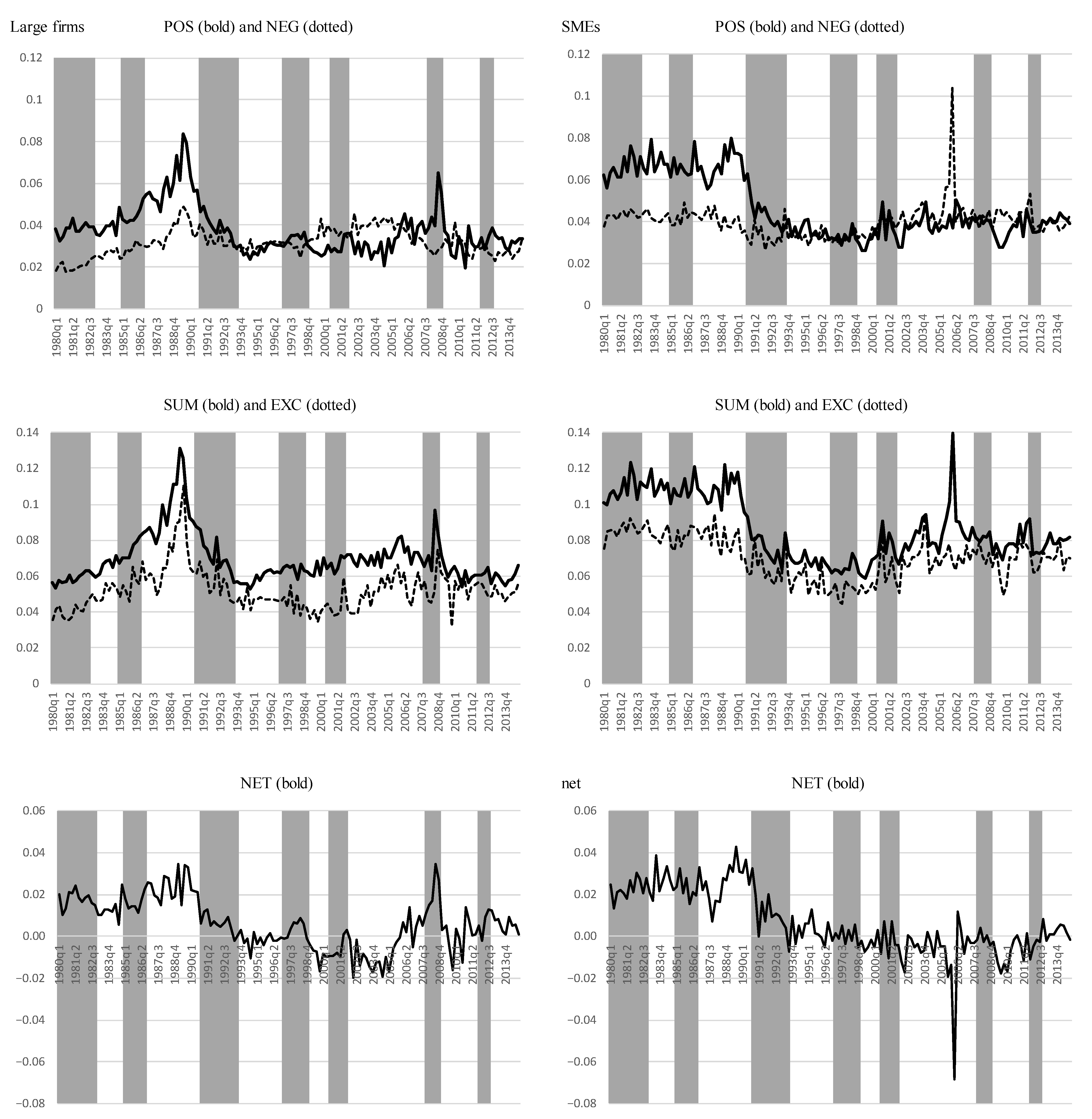
5.1. Extent of Credit Reallocation During Economic Downturns

We start by graphically depicting developments in reallocation for interest-bearing debt over the observation period in Figure 2 to capture the overall trend in credit reallocation in Japan. There are a few notable features. First, in the late 1980s, the level of credit reallocation, which is measured with credit reallocation (SUM) and excess credit reallocation (EXC), was much higher than in the other subperiods. Then, following the collapse of the asset price bubble in the early 1990s, SUM and EXC dropped dramatically in the subsequent recession. Their decline was so substantial and persistent that it was only after the 2000s that they recovered to their previous level. Second, the sharp decline in SUM and EXC in the 1990s, followed by a long period of low levels of these measures, was mainly driven by the stagnant credit creation in terms of POS.
Next, we examine how the five reallocation measures for debt instruments differ depending on the state of the economy. Table 1 presents the results for the comparison between short-term recessions and expansions and the results for the comparison between the three subperiods—before, during, and after the Lost Decade. In panel (a), we focus on interest-bearing debt. Two notable features stand out. First, for large firms, the EXC is significantly smaller during recessionary periods than during expansionary periods, although the difference is not clear for SMEs. Second, focusing on longer periods, we find that for both large firms and SMEs, both SUM and EXC are significantly smaller for the Lost Decade than for the subperiods before and after the Lost Decade taken together.
In panel (b), we implement the same set of comparisons using an alternative debt measure of bank loans because some parts of Hypotheses 1 and 1′ are based specifically on banks’ behavior of lending to borrowing firms. The results confirm the findings from panel (a). That is, for large firms in short-term recessions, the SUM and EXC are significantly smaller in recessions than in expansions. And for both large firms and SMEs in the long-term downturn, both SUM and EXC are substantially smaller for the Lost Decade than for the other subperiods.
Overall, our results in this subsection indicate that the extent of reallocation as measured with EXC or SUM is smaller in short-term recessions than in expansions. This finding is inconsistent with Hypothesis 1 but is consistent with Hypothesis 1′. Further, examining the extent of reallocation during the long-term economic downturn, the results favor Hypothesis 1′ over Hypothesis 1. Both SUM and EXC are significantly smaller for the Lost Decade than the subperiods before and after the Lost Decade. Note, however, that we have only provided a rough sketch of the examination of the hypotheses in that we did not account for the severity of recessions.
Further, we briefly consider the extent to which the above results may change when firms that newly entered or exited the market are included. As mentioned above, the data that allow us to include entering and exiting firms and cover the entire period are not available. Using a more limited data set including entering and exiting firms but covering only the period from 1999 to 2014 (see Appendix B), we find that the signs on the differences between the reallocation measures in expansionary and recessionary periods are the same regardless of whether we include or exclude entering and exiting firms. We therefore conclude that ignoring firms’ entries and exits does not appear to substantially bias the results. The detailed results are provided in Appendix D.

5.2. Correlation Between Reallocation Measures and Economic Conditions

Next, we estimate the correlation coefficients between the reallocation measures for interest-bearing debt and the aggregate economic indicators. Table 2 shows the correlation coefficients. We find that both SUM and EXC are positively correlated with some of the lagged, contemporaneous, and leading GDP and DI variables and that the credit reallocation is procyclical. The credit creation as measured by POS is procyclical for both large firms and SMEs and across different aggregate economic conditions. Specifically, while some of the contemporaneous and leading correlation coefficients are insignificant, the correlation coefficients between POS and all the lagged GDP and DI variables are statistically significant and positive. For credit destruction (NEG), no consistent signs on the correlation coefficients with lagged or leading GDP variables are observed; while the correlation coefficients are significantly positive for some of the leading GDP variables, and for some of the lagged GDP variables, they are significantly negative. In contrast, the correlation coefficients between NEG and DI that are significant are all positive.
To summarize, the SUM and EXC are positively correlated with the lagged values of aggregate economic conditions, indicating that the extent of credit reallocation is smaller during economic downturns than during expansionary phases. This is due mostly to the smaller POS in recessions.

5.3. Vector Autoregression

We employ the VAR to measure the impact of negative aggregate shocks on the extent of credit reallocation for interest-bearing debt as another way to examine Hypotheses 1 and 1′.15 Starting with large firms, Figure 3 indicates that both when focusing on GDP and when focusing on DI, an adverse shock results in a decrease in the extent of credit reallocation: SUM and EXC both show a negative response that is statistically significant at the 5% level around 5 to 10 quarters after an adverse shock. In addition, POS falls significantly for four to five quarters after a negative shock. In contrast, the response of NEG is not statistically significant.
Next, Figure 4 shows the corresponding results for SMEs. Overall, the responses of the reallocation measures are smaller than in the case of large firms. That is, while POS falls significantly in response to a negative shock to real GDP or the DI, the decline in SUM is significant only in the case of a negative shock to the DI, and all the other responses are not significant.16
Taken together, the results indicate that the extent of credit reallocation as measured with SUM or EXC decreases following a negative shock to the economy, and this decline is mostly driven by the drop in the extent of credit creation, that is, POS. This is in line with Hypothesis 1′, which predicts that the extent of reallocation and credit creation will be smaller in recessions. Conversely, we do not find evidence that supports Hypothesis 1 in which credit destruction increases due to the break-up of lender–borrower relationships during recessions. In fact, the results above show that negative aggregate shocks do not increase credit destruction (NEG) in Japan, which is the opposite of the findings for Korea and the United States. They actually find that credit destruction significantly increases during recessions (Herrera et al. 2011; Hyun and Minetti 2019).
In an additional examination using a variance decomposition, we confirm the substantial contribution of aggregate shocks to fluctuations in the credit reallocation and those in the credit creation. Figure 5 shows the results for large firms. Negative shocks to real GDP and DI have a substantial impact on the variation in the credit reallocation. Specifically, these shocks explain 11–14% of the variation in SUM and 7–8% of that in EXC. We interpret that this substantial effect is attributed to the impact of shocks to real GDP and DI on the fluctuation in the credit creation, because these shocks explain 24–31% of the variation in POS. In Figure 6, we observe similar results for SMEs, although the impact is smaller than for large firms. The shocks to real GDP and DI explain 4–12% of the variation in SUM and EXC, and they explain 9–22% of the variation in POS. These results indicate that negative aggregate shocks have a substantial effect on credit reallocation (SUM and EXC) and that this effect is primarily driven by the impact of negative shocks on the variation in credit creation (POS).

6. Results for the Efficiency of Credit Reallocation

Having examined the extent of credit reallocation in the previous section, we examine in this section the efficiency of credit reallocation and test Hypotheses 2, 3, and 3′. We achieve this by focusing on the link between credit reallocation and firm-level productivity.

6.1. Summary Statistics

Table 3 presents the summary statistics for the variables used for analysis in this section. The statistics are for the entire sample and for the subperiods. The dependent variable, debt growth, is the rate of change either in a firm’s interest-bearing debt or in its loans from banks and ranges from −2 to +2. The average values for the entire period are −0.007 and −0.010, respectively. These values indicate that firms’ total borrowing and bank loans decreased slightly over the course of our observation period.

6.2. Baseline Estimation

We start with our baseline estimation using Equation (6) from Section 4.2.17 The results are shown in Table 4. The key variable of interest is l n T F P t 1 , the one-period lag of the natural log of TFP. In Column (1), we find that the coefficient for l n T F P t 1 is positive and significant, indicating that the growth rate of debt is larger for more productive than for less productive firms, which means that the credit flows from low-productivity to high-productivity firms. This observation is consistent with Hypothesis 2 that credit reallocation is efficiency-enhancing. We obtain a somewhat different result when the DI instead of real GDP is used in the estimation: in Column (2), the coefficient for l n T F P t 1 is insignificant.
Next, to investigate under what circumstances we find a significantly positive coefficient for l n T F P t 1 , we conduct estimations using Equation (7) in which the interaction term between TFP and the cyclical component of one of the two aggregate economic indicators (real GDP or the DI) is added. Columns (3) and (4) show the results, which differ somewhat from each other. In Column (3), the coefficient for l n T F P t 1 is positive and significant and the interaction term is not significant, while in Column (4), both l n T F P t 1 and the interaction term have positive and significant coefficients. Based on the result in Column (4), we can say that reallocation is less efficiency-enhancing in economic downturns. When the economy is in a severe downturn to mark the lowest DI of −49, the marginal effect of l n T F P t 1 is −0.007 (0.00471 + 0.000239 × (−49)). In this situation, a one-standard-deviation decrease in l n T F P t 1 (0.412) increases credit growth by about 0.3 percentage points, which is an economically substantial efficiency-reducing reallocation.
From these results, we infer the following: First, generally speaking, productivity has a positive impact on the growth of credit that is consistent with Hypothesis 2. Second, the positive impact becomes smaller in recessions when we use the interaction term of TFP and the DI, indicating that reallocation is less efficiency-enhancing and turns negative when the depth of the recession is severe that indicates it is efficiency-reducing. These results are consistent with Hypothesis 3′ rather than Hypothesis 3. Note, however, that the evidence supporting Hypothesis 3′ is not that strong since we find no evidence for the hypothesis when using the interaction term of TFP and the cyclical component of GDP.
In order to further examine Hypotheses 3 and 3′, we therefore look at the impact of Japan’s long-term economic stagnation during the Lost Decade rather than the impact of short-term recessions. For the estimation, the results are shown in Columns (5) to (10). Interestingly, the coefficients for l n T F P t 1 differ substantially across the subperiods. For the subperiod before the Lost Decade (i.e., the 1980s), the coefficients for l n T F P t 1 are positive and significant, as shown in Columns (5) and (6). In contrast, for the Lost Decade, the coefficients are significantly negative (Columns (7) and (8)). Finally, for the subperiod after the Lost Decade (Columns (9) and (10)), the coefficients become positive again but are smaller than before the Lost Decade. In sum, we find that credit reallocation was not only less efficiency-enhancing in the Lost Decade than in other periods but also efficiency-reducing. During this period, a one-standard-deviation decrease in l n T F P t 1 increased the credit growth rate by about 0.1 percentage points ((Columns (7) and (8)). This finding is again consistent with Hypothesis 3′ rather than Hypothesis 3.
It is worth taking a brief look at the results for the other explanatory variables used as controls. They are generally consistent with expectations. The coefficients for l n A s s e t s t 1 are negative, while those for S a l e s _ g r o w t h t 1 are positive, indicating that smaller and fast-growing firms tend to have a larger demand for funds. Next, the coefficients for firms’ return on assets (ROA), which represents their profitability, are negative and significant. These coefficients simply reflect that profitable firms tend to have abundant internal financial resources to meet their needs and therefore are less likely to demand external funding. Finally, the coefficients for C a p i t a l _ r a t i o t 1 , which represents firms’ creditworthiness and the agency costs they face, are positive and significant, indicating that firms with a high capital ratio are more likely to be able to obtain outside funding than firms with a low capital ratio.
Since some parts of Hypothesis 3′ are about banks’ lending behavior rather than about firms’ financing overall, we also implement the same set of estimations using an alternative dependent variable of loans extended by banks. The results are shown in Table 5 and are similar to those in Table 4, although there are a few notable differences. For the entire period, the coefficients for l n T F P t 1 are positive and larger than those in Table 4, indicating that the extent to which the reallocation of bank loans was efficiency-enhancing was more pronounced than the extent to which the reallocation of interest-bearing debt was efficiency-enhancing. In the subperiod analyses, the most notable difference from Table 4 is that the coefficients for productivity are insignificant for the Lost Decade but not significantly negative. We can therefore say that during the Lost Decade, the reallocation of bank loans was less efficiency-enhancing than in other periods, but we cannot say that it was efficiency-reducing.
The result that the reallocation of bank loans was not efficiency-reducing but that the reallocation of interest-bearing debt was efficiency-reducing may contradict the contention in some studies (e.g., Peek and Rosengren 2005; Caballero et al. 2008) that Japanese banks followed perverse incentives to extend loans to nonviable firms during the Lost Decade. It could be that the reallocation of bank loans was efficiency-reducing only for a specific category of firms, an issue which we will examine in Section 6.4.

6.3. Estimations Including Exiting Firms

In the baseline estimation, we limited our focus to surviving firms and excluded those that exited or entered during the observation period. However, credit reallocation for these entering and exiting firms may differ from that for surviving firms. In order to examine this issue, we implement an estimation that includes not only surviving but also exiting firms by using the data set we introduced in Section 3.2 and Appendix B to measure the extent of reallocation. Note that due to data limitations, this estimation covers a shorter period from 2000 to 2013 than the baseline estimation.
Table 6 shows the results. Columns (1) to (4) present the results of the estimations including exiting firms. The coefficients for l n T F P t 1 are all positive and significant, supporting Hypothesis 2. Meanwhile, the coefficients for the interaction terms in Columns (3) and (4) are not significant, meaning that we cannot say whether Hypothesis 3 or 3′ is supported. Columns (5) to (8) show the estimation results for surviving firms only. The results are qualitatively similar to those in Columns (1) to (4). That is, the coefficients for l n T F P t 1 are all positive and significant, and those for the interaction terms are all insignificant. In sum, including exiting firms in the data set does not qualitatively change the estimation results or our assessment regarding which of the hypotheses are consistent with the data.
In order to further examine how the inclusion of exiting firms affects our results with regard to Hypothesis 2, we compare the productivity levels of surviving and exiting firms. If the productivity of surviving firms is higher than that of exiting ones, the process of firm survival and exit will increase the average productivity level that would provide further supporting evidence for Hypothesis 2. Column (11) shows the results of t-tests for the difference between the means of explanatory variables for firms that survived and those that exited. The difference in average TFP between surviving and exiting firms is not statistically significant. This result indicates that a decline in the amount of credit outstanding due to the exit of firms neither increases nor decreases average productivity and neither supports nor rejects Hypothesis 2.

6.4. Examination of the Reasons for Efficiency-Reducing Reallocation in the Lost Decade

The results in Table 4, Table 5 and Table 6 showed that credit reallocation is generally efficiency-enhancing; moreover, the extent to which reallocation is efficiency-enhancing is smaller in recessions, and reallocation was in fact efficiency-reducing during the Lost Decade. However, it is still unclear why reallocation was efficiency-reducing during the Lost Decade. As posited in the latter part of Hypothesis 3′, there are two possible explanations, focusing on financial constraints on productive firms and financial assistance to unproductive and nonviable firms.
The first explanation is based on the conjecture that productive firms have a larger demand for loans than less productive firms and therefore are more likely to be financially constrained in a recession (Barlevy 2003). Based on this line of reasoning, we predict that small or highly leveraged firms, which are more likely to be financially constrained in recessions, tend to experience efficiency-reducing credit reallocation. The second explanation focuses on firms that are likely to receive financial assistance when they are unproductive and nonviable (Dewatripont and Maskin 1995; Berglöf and Roland 1997; Fukuda et al. 2007). We predict that large firms, which are often too big to fail or cause a dynamic commitment problem for lenders, receive financial assistance and experience efficiency-reducing reallocation in economic downturns.
With these two potential explanations in mind, we estimate specification (9) for two different sets of subsamples: firm size and capital ratio. If the first explanation holds, small firms or highly leveraged firms will have experienced efficiency-reducing credit reallocation during the Lost Decade, that is, we will observe a negative β 2 for these firms. In contrast, large firms will have experienced efficiency-reducing reallocation if the second explanation fits reality.
Figure 7 shows the results in four different panels that display the coefficients for l n T F P t 1 in the estimation for debt growth and bank loan growth during the Lost Decade. The left panels use debt growth as the dependent variable. The top left shows the coefficient estimates for the three subsamples based on firm size, i.e., small, large, and very large firms. While the coefficient for very large firms is negative and significant, those for small and large firms are insignificant. These results are more consistent with the second explanation, based on which we predicted that very large firms, that is, firms that are too big to fail or cause dynamic commitment problems for lenders will have efficiency-reducing credit reallocations (Dewatripont and Maskin 1995; Berglöf and Roland 1997; Fukuda et al. 2007). Next, we divide firms into quartiles in terms of their capital ratio and conduct estimations for each subsample. The results are shown in the bottom left panel. Only in the estimation for firms in the third (i.e., second highest) quartile in terms of their capital ratio do we obtain a negative and significant coefficient, while the other three estimations yield insignificant coefficients. This is not consistent with the first explanation, which predicts a negative coefficient for firms with low a capital ratio. Finally, the panels on the right display the growth of bank loans as the dependent variable and obtain qualitatively similar results as in the left panels.
The above results are consistent with the second explanation that financial institutions continued to extend loans to financially assist unprofitable and nonviable firms. However, they still do not provide conclusive evidence that the financial assistance provided by banks during the Lost Decade was efficiency-reducing, as suggested by studies on zombie firms such as that by Caballero et al. (2008).
The square dots represent the coefficient estimates, while the vertical lines represent the 95% confidence intervals.
We therefore implement another subsample analysis for the Lost Decade that distinguishes between firms that received financial assistance and those that did not. We follow Caballero, Hoshi, and Kashyap to detect whether firms received financial assistance. Details of the procedure are provided in Appendix E.18
The results of this analysis are shown in Figure 8 and differ depending on whether we use overall debt (left panel) or bank loans (right panel). The left panel shows that the coefficients for both firms that received financial assistance and those that did not are significantly negative and very similar in size. In contrast, in the right panel, the coefficients for the two groups of firms differ in that reallocation was efficiency-reducing for firms that received assistance, while it was neither efficiency-enhancing nor efficiency-reducing for firms that did not receive assistance. As the focus of the examination is on the assistance extended by financial institutions, what is of interest here is the result for bank loans. Based on this result, we can say that reallocation was efficiency-reducing when firms received financial assistance during the Lost Decade, providing support for the explanation based on the last sentence in Hypothesis 3′.

7. Conclusions

This study focuses on the reallocation of credit in Japan across both large firms and SMEs spanning a period of more than three decades. We first examined the extent of credit reallocation, especially when the economy was in a downturn. We then investigated if reallocation was efficiency-enhancing, that is, if credit flows from less productive to more productive firms. We obtained the following three major findings. First, the extent of credit reallocation is smaller in recessions than in expansions that is attributable to the decreasing extent of credit creation. Second, this tendency was more pronounced during the Lost Decade. Third, credit reallocation generally is efficiency-enhancing, but it is less efficiency-enhancing in recessions and becomes efficiency-reducing during the Lost Decade, possibly due to financial assistance to large but low-quality firms. These findings together suggest that the inefficient credit reallocation during the Lost Decade was characterized by efficiency-reducing reallocation for large firms.
Our finding of the efficiency-reducing reallocation during the Lost Decade is consistent with the stories suggested by the studies on zombie lending. These studies have shown that the central mechanism behind zombie lending is that weakly capitalized banks have an incentive to extend credit to insolvent firms in order to avoid their realization of capital losses (Peek and Rosengren 2005; Caballero et al. 2008). To prevent such distorted behavior of banks, there are two possible policy measures. The first such measure is the recapitalization of banks. Bruche and Llobet (2014) show in their theoretical model that undercapitalized banks have an incentive to evergreen loans to insolvent borrowers. If the government injects enough capital into banks to meet capital requirements for these banks, such perverse incentives for banks should be considerably alleviated. In reality, however, Giannetti and Simonov (2013) show that the capital injections implemented by the Japanese government during 1998–2004 were insufficient, banks remained undercapitalized and zombie lending continued to increase. The second policy measure is stronger bank supervision. The empirical studies show that strengthening bank inspections and audits reduces lending to zombie firms while it increases loans to productive firms (Passalacqua et al. 2021; Bonfim et al. 2022). However, it was only around the 2000s did the Financial Services Agency of Japan introduce stringent bank inspection rules and encouraged banks to write-off a massive amount of nonperforming loans. This belated policy response helped the practice of zombie lending to prevail.
While our results provide useful insights into the efficiency of credit reallocation during economic downturns and possible policy responses, the research could be extended in a number of ways. For example, an examination of the interaction between the reallocation of interest-bearing liabilities and the reallocation of physical inputs (labor and capital) or of other financial resources (equity and internal funds) may provide further insights on the functioning of resource reallocation in the economy. Given that the amount of research on the reallocation of financial resources is still quite limited relative to the abundant literature on job and capital reallocation, an interesting avenue for future research would be to examine the substitutive or complementary relationships between the reallocation of different resources. Another important issue for future research is to examine what firms determine the extent and efficiency of credit reallocation. For example, the extent and efficiency of credit reallocation could be driven by the behavior of a limited number of large firms. Or it could be driven by unlevered firms (i.e., firms that hold no debt during the period). There has been a growing interest in the latter type of firms (see, e.g., El Ghoul et al. 2018), and the share of such unlevered firms has been on the rise in Japan in recent years. It would be interesting to examine the role of such firms in the context of credit reallocation.

Author Contributions

Conceptualization, K.S. and I.U.; methodology, K.S. and I.U.; software, K.S. and I.U.; validation, K.S. and I.U.; formal analysis, K.S. and I.U.; investigation, K.S. and I.U.; resources, I.U.; data curation, K.S.; writing—original draft preparation, I.U.; writing—review and editing, K.S. and I.U.; visualization, K.S. and I.U.; supervision, K.S. and I.U.; project administration, K.S. and I.U.; funding acquisition, K.S. and I.U. All authors have read and agreed to the published version of the manuscript.

Funding

The financial support provided by the JSPS KAKEN Grants 16K03757 and 18K01677 and the Ishii Memorial Securities Research Promotion Foundation is gratefully acknowledged.

Data Availability Statement

The dataset used in this study, the Quarterly Financial Statements Statistics of Corporations by Industry (QFSSC), is not publicly available because the use of data requires permission from the Ministry of Finance in Japan.

Acknowledgments

We are grateful to the editor and three anonymous referees for their valuable comments. We also thank Masaru Hanazaki (discussant), Masahisa Fujita, Masayuki Morikawa, Hiroshi Ohashi, Yasuo Goto, Raoul Minetti, Arito Ono, Hirofumi Uchida, Daisuke Miyakawa, Daisuke Tsuruta, Kaoru Hosono, Wako Watanabe, Yoshiaki Ogura, Ralph Paprzycki, Tadanobu Nemoto, Peng Xu, Masazumi Hattori, Yuta Takahashi, Naoki Takayama, and participants of the Japan Society for Monetary Economics Meeting and the RIETI Study Group on Corporate Finance and Firm Dynamics for their valuable comments. We also thank YoungGak Kim for providing us with a code for calculating the total factor productivity.

Conflicts of Interest

The authors declare no conflicts of interest.

Appendix A. Firm-Level Data from the Quarterly Financial Statements Statistics of Corporations by Industry

The Quarterly Financial Statements Statistics of Corporations by Industry (QFSSC) is a survey of business corporations whose headquarters are located in Japan. The QFSSC started in the fourth quarter of the fiscal year 1949, and firm-level data in electronic form are now available to researchers (after a time-consuming application process) for the period from the first quarter of the fiscal year 1980.
The QFSSC contains information on individual corporations such as their balance sheets, employment, industry, geographic location, and transactions in fixed assets. They cover all manufacturing and non-manufacturing industries, although we exclude finance and insurance from the analysis. The QFSSC consists of two parts: a part that targets all large corporations, and a part that consists of a sample of smaller firms.
There was a substantial change in the fiscal year 2009 in the way that firms were chosen for the survey. Up to the fourth quarter of the fiscal year 2008, the first part of the survey targeted all corporations with paid-in capital of JPY 600 million or more, and observations consisted of all such corporations that responded to the questionnaire, while the second part consisted of a sample of smaller firms that was subdivided into those with paid-in capital ranging from JPY 100 to 600 million and those with paid-in capital of less than JPY 100 million. In the second part, sampling was conducted in a manner such that among the firms in the JPY 100 to 600 million bracket, larger firms were more likely to be chosen, while among firms with paid-in capital of less than 100 million, those were chosen randomly regardless of their capital size. All smaller firms with paid-in capital of less than JPY 600 million that were surveyed received a questionnaire for four quarters from the first to the fourth quarter of the fiscal year, while all larger corporations always received a survey questionnaire.
Since the first quarter of the fiscal year of 2009, the first part has targeted all corporations with paid-in capital of JPY 500 million (instead of JPY 600 million) or more. On the other hand, the second part is no longer subdivided. Instead, firms are randomly chosen from the pool of firms with paid-in capital of less than JPY 500 million. All firms with less than JPY 500 million of paid-in capital that are surveyed receive a questionnaire for eight quarters (two years), with half of the firms replaced in the first quarter of each fiscal year. As before, all larger corporations continue to always receive the survey questionnaire.

Appendix B. Construction of the Data Set That Incorporates Firms’ Entries and Exits

In this appendix, we explain the procedure we use to identify the timing of the entries and exits of firms in the QFSSC. The QFSSC does not have information on the age of the firm or the year that it exited from the market. To obtain this information, we use another data source provided by the Teikoku Databank (TDB) that is one of Japan’s largest private credit research companies. TDB has a comprehensive database called COSMOS2 that contains information on more than four million firms in Japan.19 From the database, information on corporations with 40 employees or more from 1999 onward is available to researchers.
Since the QFSSC and the data set extracted from COSMOS2 do not use the same identification numbers for firms, we use their names, reporting years, the amounts of paid-in capital, and the prefectures in which they are located to match observations in the two data sets. The total number of observations that we can match for the period from 1999 and 2014 is 695,599.
Using this data set, we identify the year a firm first showed up and the year it was last recorded in the data and regard these years as the firm’s years of entry and exit. If this entry year in COSMOS2 is the same as the year a firm first showed up in the QFSSC, we identify this as the firm’s entry year. Similarly, we define a firm’s exit year as its exit year when the year in COSMOS2 matches the year the firm responded to the QFSSC survey for the last time.
In the analysis, we use this data set to examine the impact of firms’ entries and exits on the extent of credit reallocation. We also test whether including these entering and exiting firms changes the estimation results on the extent to which credit reallocation is efficiency-enhancing.

Appendix C. Calculation of TFP

An important variable that we construct represents firms’ productivity. Firm-level TFP can be calculated using one of two different methods: subtracting the cost share of each input from the output or estimating a production function and using the parameters obtained from the estimation. In order to have as many observations as possible, we employ the first approach for our analysis, which is also used by Foster et al. (2016) that is one of a limited number of studies on the relationship between resource reallocation and TFP. However, this method requires the possibly unrealistic assumption of perfect competition.
Among a variety of approaches based on the latter method, researchers most frequently use the control function approach that was originally proposed by Olley and Pakes (1996) and developed by Levinsohn and Petrin (2003) and Ackerberg et al. (2015), among others. The reason we do not employ this approach is that it requires lagged values and we would need to drop a large number of observations for SMEs, since for many of them, the lagged values are not available. Following the work of Good et al. (1997), Aw et al. (2001), and Fukao and Kwon (2006), we define the TFP level of firm f at time t in a certain industry relative to the TFP level of a representative firm in the base year 0 in that industry based on the following equation:
l n T F P f t = l n Y f t l n Y ¯ t + s = 1 t l n Y s ¯ l n Y s 1 ¯ i = 1 n 1 2 S i f t + S i t ¯ l n X i f t l n X i t ¯ + s = 1 t i = 1 n 1 2 S i s ¯ S i s 1 ¯ l n X i s ¯ l n X i s 1 ¯
where Y f t , S i f t , and X i f t denote the gross output (sales) of firm f at time t, the cost share of factor i for firm f at time t, and firm f’s input of factor i at time t, respectively. Variables with an upper bar denote the industry average of that variable. As input factors, we include capital, labor, and intermediate inputs. The details of the construction of the output and input factor variables are as follows:
Output
We use each firm’s total sales for nominal gross output. We construct the output deflator for a particular year by dividing the industry-level nominal gross output by the real gross output obtained from the JIP database. We calculate the deflator annually rather than quarterly because the JIP database provides value-added statistics only at an annual frequency.
Labor
For L i t , we calculate the total hours worked based on the following formula:
L i t = N u m b e r   o f   E m p l o y e e s i t Y e a r l y   H o u r s   W o r k e d s t .
We obtain the firm-level number of employees from the QFSSC. We also calculate industry-level yearly hours worked per person from the hours worked and the number of employees in the JIP database.
Capital
We calculate real capital (non-land tangible assets) K i t at market prices from the information on the nominal book value of a firm’s capital in the QFSSC, K N i t . We first calculate the industry-level series of non-land tangible assets in terms of their market value, K s y , for a particular year y , using the following formula:
K s 0 = K N s 0 P I N V E S T s 0
K s y = 1 δ s y K s y 1 + I N V E S T s y P I N V E S T s y ,   t   =   1 ,   Y ,
where K N s y is the industry-level nominal amount of non-land tangible assets outstanding measured at the end of y, P I N V E S T s y is the industry-level investment deflator, I N V E S T s y is the nominal amount of investment in non-land tangible assets, and δ s y is the industry-level depreciation rate. We set 1975 as the starting year, that is, y = 0. All information for the above calculations is obtained from the JIP database and the Annual Financial Statements Statistics of Corporations by Industry. The Annual Financial Statements Statistics of Corporations by Industry (AFSSC) are annual statistics on firms’ financial statements that, like the QFSSC, are compiled by the Ministry of Finance. We use the AFSSC instead of the QFSSC since we construct the variable R a t i o at an annual frequency. We obtain the industry-level market-to-book value ratio and the firm-level amount of real non-land tangible assets at market prices using the following formula:
R a t i o s y = K s y K N s y
K i t = R a t i o s y K N i t .
Intermediate inputs
We calculate the real firm-level input of intermediate goods, M i t , using the following formula:
M i t = S a l e s   C o s t i t + S a l e s   A d m i n i s t r a t i v e   E x p e n s e i t ( P e r s o n n e l   C o s t i t + D e p r e c i a t i o n i t ) P M s y
where P M s y is the industry-level intermediate input deflator in year y that is calculated from the industry-level nominal intermediate inputs and real intermediate inputs obtained from the JIP database.
We also need to specify the industries that we use to calculate the firms’ TFP based on Equation (A1). In principle, we use the industry classifications used in the QFSSC. However, we combine some of the categories to have consistent industry classifications before and after the revision of classifications in the QFSSC in 2009. We also use this combination in order to be able to match the classifications with those used in the JIP database. The following is a list of industry classifications (which roughly follow the Japan Standard Industrial Classification) used for the analysis.
Industry Classification Used for the Analysis
Industry CodeName of Industry
1Agriculture, forestry, and fishery
10Mining and quarrying of sand and gravel
15Construction
18Food processing
20Textiles and clothing
22Wood and wood products
24Pulp and paper
25Printing and allied industries
26Chemicals
27Petroleum and coal products
30Ceramic products
31Iron and steel
32Non-ferrous metals
33Metal products
34General and precision machinery
35Electrical and IT machinery
36Automobiles and parts
38Other transportation machinery
39Other manufacturing
40Wholesale
49Retail
59Real estate
60Information and telecommunication
61Land, water, and other transportation
70Electricity, gas, heat supply, water
75Other services

Appendix D. Impact of Including Entering and Exiting Firms on the Extent of Credit Reallocation

In Section 5.1, we limited the scope of the analysis to firms for which observations at both ends of the interval between time t − 1 and t are available. This limitation means that we fail to take account of the impact of firms that have newly entered or exited the market, possibly resulting in a downward bias in our reallocation measures. We measure the extent of possible biases in the extent of credit reallocation. We also examine how large these biases are in the extent of reallocation during economic downturns and upturns. In this appendix, we use the data set described in Section 3.2 and in Appendix B.
Panel (a) of Appendix D Table A1 shows the mean values of the five credit reallocation measures by firm size for the period 2000–2014 when entering and exiting firms are included and when they are excluded. We employ interest-bearing debt as the debt instrument. Since the absolute growth rate of credit for entering and exiting firms is 2 in most cases, which is the maximum possible value, including these firms in the data set will likely increase POS, NEG, and SUM.20 And indeed, in the table, the values of these three measures in the second row are larger than those in the first row. We also find that the difference is substantially larger for SMEs than for large firms, reflecting the fact that most entering and exiting firms are small in size.
Next, we examine the changes in the extent of credit reallocation during expansionary and contractionary phases. In each of the two data sets, that is, the data set without entering and exiting firms and the data set including these firms, we compare the extent of credit reallocation between expansionary and contractionary periods.
In panel (b), we show the results. Regardless of firm size, the signs of the differences between the reallocation measures in expansionary and recessionary periods are the same regardless of whether the data set includes or excludes entering and exiting firms. The statistical significance of these differences is also similar between the two data sets. To summarize, inclusion of entering and exiting firms in the analysis increases the level of credit reallocation, especially for SMEs. However, this does not appear to qualitatively change our results regarding the extent of credit reallocation during an economic downturn. Thus, ignoring firms’ entries and exits in our analysis does not appear to substantially bias the results.
Table A1. Extent of credit reallocation for interest-bearing debt including/excluding entering and exiting firms. This table presents the extent of credit reallocation for interest-bearing debt and (a) compares each of the reallocation measures when entering and exiting firms are excluded and when they are included. It also (b) compares the extent of reallocation between expansionary and recessionary periods. Definitions of variables are provided in Section 3.2. The ***, **, and * denote significance at the 1%, 5%, and 10% levels, respectively.
(a) Results for the observation period from FY2000 to FY2014.
Large firms SMEs
POSNEGNETSUMEXCPOSNEGNETSUMEXC
2000sQ1–2014Q4 (excl. entry & exit)0.0330.034−0.0000.0670.0512000sQ1–2014Q4 (excl. entry & exit)0.0380.043−0.0050.0810.069
2000sQ1–2014Q4 (incl. entry & exit)0.0330.035−0.0010.0680.0532000sQ1–2014Q4 (incl. entry & exit)0.0410.053−0.0110.0940.073
H0: Excl. = Incl. ***********H0: Excl. = Incl.***************
(b) Results when distinguishing between expansions and recessions.
Large firmsSMEs
2001sQ1–2014Q4 (excl. entry & exit)POSNEGNETSUMEXC2001sQ1–2014Q4 (excl. entry & exit)POSNEGNETSUMEXC
Expansions0.0320.034−0.0020.0660.052Expansions0.0380.044−0.0050.0820.069
Recessions0.0370.0310.0060.0680.050Recessions0.0380.041−0.0030.0790.068
Difference−0.0050.003−0.009−0.0020.002Difference−0.0000.003−0.0030.0020.001
H0: Expansions = Recessions******H0: Expansions = Recessions
2001sQ1–2014Q4 (incl. entry & exit)POSNEGNETSUMEXC2001sQ1–2014Q4 (incl. entry & exit)POSNEGNETSUMEXC
Expansions0.0320.035−0.0030.0670.054Expansions0.0410.054−0.0120.0950.073
Recessions0.0370.0330.0040.0700.051Recessions0.0410.048−0.0080.0890.073
Difference−0.0050.002−0.007−0.0020.002Difference0.0010.005−0.0040.0060.000
H0: Expansions = Recessions****H0: Expansions = Recessions

Appendix E. Identification of Firms That Received Financial Assistance

The construction of the variable to identify the firms that received financial assistance follows the identification of zombie firms in the work of Caballero et al. (2008) (hereafter CHK). In order to identify zombie firms using the QFSSC, we limit observations to firms for which financial statement information for all four quarters in a fiscal year is available. We then sum a firm’s interest payments and profits over the four quarters in a fiscal year. Moreover, we use a firm’s amount of debt outstanding at the end of the fiscal year.
CHK define zombie firms in relation to the hypothetical lower bound for interest payments ( R i t ) for the highest quality borrowers that they define as follows:
R i t = r s t 1 B S i t 1 + 1 5 j = 1 5 r l t j B L i t 1 + r c b min   over   last   5   years ,   t × B o n d s i t 1 ,
where B S i t , B L i t , and B o n d s i t are short-term bank loans, long-term bank loans, and total bonds outstanding (including convertible bonds) of firm i at the end of fiscal year t, respectively. The interest rates r s t and r l t are the average short-term and long-term prime rates for fiscal year t, respectively, and r c b min   over   last   5   years ,   t is the minimum observed rate on any convertible corporate bond issued over the previous five years prior to t. CHK define zombies as firms whose interest payments R i t were lower than R i t . The basic idea is that troubled firms must have received substantial interest relief to be making lower interest payments than healthy firms.

Notes

1
Note that there is also a strand of studies that examine credit reallocation among banks rather than among firms (Dell’Ariccia and Garibaldi 2005; Contessi and Francis 2013).
2
In addition to these studies, Li et al. (2023) and Saini and Ahmad (2024) empirically examine the characteristics and cyclicality of credit reallocation for China and India, respectively. More recently, Cuciniello (2024) investigated the credit allocation to businesses in Italy during the COVID-19 crisis.
3
All of these theoretical studies on resource reallocation focus on economic downturns. The focus on and interest in economic downturns among researchers date back to Schumpeter (1934), who argued that the main function of recessions lies in the liquidation and reallocation of resources.
4
For evidence regarding the duration of firm–bank relationships in Japan, among other countries, see Table 4.1 in the work of Degryse et al. (2009).
5
In a similar vein, this logic applies to firms with high leverage. In later analyses, we focus not only on small firms but also firms with low capital ratios to examine Hypothesis 3′.
6
Meanwhile, Bruche and Llobet (2014) argue that lenders’ limited liability may lead to possible distortions in the credit market that result in lenders providing financial assistance to nonviable borrowers in recessionary times.
7
Other studies have empirically examined the existence of zombie lending in countries other than Japan as well. In Europe, Bonfim et al. (2022) for Portugal, and Schivardi et al. (2022) for Italy show that unhealthy banks evergreened loans to zombie firms during the global financial crisis and subsequent sovereign debt crisis in Europe. In Asia, Chopra et al. (2021) show that undercapitalized banks increased lending to zombie firms after an asset quality review (AQR) in India, and Li and Ponticelli (2022) show that zombie lending occurred in areas with less specialized courts in China. Acharya et al. (2022) provide a more detailed survey of the recent research in this area.
8
The JIP database has been produced by RIETI in collaboration with the Institute of Economic Research at Hitotsubashi University. For details, see https://www.rieti.go.jp/en/database/jip.html.
9
This is because the QFSSC has covered this industry only for a limited period (since the first quarter of the fiscal year 2008).
10
Note that we have g f t = 0 when the firm has zero debt outstanding at both time t − 1 and t.
11
Among the previous studies that examine the cyclicality of credit reallocation, Herrera et al. (2011), Dell’Ariccia and Garibaldi (2005), and Hyun and Minetti (2019) measure correlation coefficients, while Dell’Ariccia and Garibaldi (2005) adopt the VAR. Note, however, that both of these methods examine the extent of reallocation when the economy is in a short-term recession and not when it is experiencing long-term stagnation.
12
The DI is based on firms’ responses in the Bank of Japan’s Tankan survey regarding how they assess their current business conditions. The DI is obtained by subtracting the percentage of firms that say current conditions are unfavorable from the percentage of those saying that they are favorable, so that a higher DI indicates better business conditions.
13
Specifically, we follow Dell’Ariccia and Garibaldi (2005) in the way we extract the cyclical components. The cyclical component of each series is defined as the deviation of the logged original values of the credit reallocation measures and those of real GDP from their Hodrick–Prescott (HP) filtered logged values, with a smoothing parameter of 1600 that business cycle studies usually use for quarterly data. The cyclical component therefore is expressed in percentage terms. To ensure that the reallocation measures are expressed in percentage terms, we adjust the original values of the credit reallocation measures by multiplying them by C s t . Note that we do not derive cyclical components for the net credit change, since it may take negative values and cannot be logged.
14
We limit the observation period to the end of the fiscal year of 2013 rather than the first quarter of 2014, which is the last period of our credit reallocation data, because some of the data we need for the calculation of our variables from the JIP database are unavailable.
15
In the VAR analysis, we perform Augmented Dickey–Fuller (ADF) tests to check for the stationarity in each time series, and the null of unit root is rejected in all cases. To select the lag length for each VAR, we adopt the lag-order selection statistics of Akaike’s information criterion (AIC). We performed lagrange multiplier (LM) tests for serial correlation on VAR residuals, and the null of no serial correlation was not rejected in all cases.
16
Throughout the two subsections focusing on correlation coefficients and VAR, we follow the convention and extract cyclical components by applying the HP filter to credit reallocation and real GDP.
17
Although the results are not shown, we checked the correlation matrix for all pairs of covariates used in the estimation in Section 6 to find no substantially correlated pairs of variables that possibly cause multicollinearity.
18
Caballero, Hoshi, and Kashyap use this procedure for the purpose of detecting zombie firms. There are several other studies that provide different definitions of zombie firms including Fukuda and Nakamura (2011), Imai (2016) and Goto and Wilbur (2019). However, we solely employ the procedure by Caballero, Hoshi, and Kashyap because their definition is simply based on the difference between a firm’s individual interest rate and the market prime rate, which is orthogonal to a change in a firm’s borrowing amount.
19
The TDB website states that the company holds information on about 4.2 million firms (see https://www.tdb.co.jp/info/topics/k170501.html, in Japanese, accessed 21 March 2021). Government statistics indicate that currently, there are 1.5 million corporations and 2.3 million proprietorships, totaling 3.8 million firms, which indicate that the TDB database covers almost the entire universe of Japanese firms.
20
The growth rate of debt ( g f t ) for an entering firm f is ( D e b t f t − 0)/0.5( D e b t f t     + 0) = 2 if D e b t f t > 0, and that for an exiting firm f is (0 − D e b t f t 1 )/0.5(0 + D e b t f t 1 ) = −2 if D e b t f t 1   > 0.

References

  1. Acharya, Viral V., Matteo Crosignani, Tim Eisert, and Sascha Steffen. 2022. Zombie Lending: Theoretical, International, and Historical Perspectives. Annual Review of Financial Economics 14: 21–38. [Google Scholar] [CrossRef]
  2. Ackerberg, Daniel A., Kevin Caves, and Garth Frazer. 2015. Identification Properties of Recent Production Function Estimators. Econometrica 83: 2411–51. [Google Scholar] [CrossRef]
  3. Aw, Bee Yan, Xiaomin Chen, and Mark J. Roberts. 2001. Firm-Level Evidence on Productivity Differentials and Turnover in Taiwanese Manufacturing. Journal of Development Economics 66: 51–86. [Google Scholar] [CrossRef]
  4. Banerjee, Ryan, and Boris Hofmann. 2018. The Rise of Zombie Firms: Causes and Consequences. BIS Quarterly Review 2018: 67–78. [Google Scholar]
  5. Barlevy, Gadi. 2003. Credit Market Frictions and the Allocation of Resources over the Business Cycle. Journal of Monetary Economics 50: 1795–818. [Google Scholar] [CrossRef]
  6. Beck, Thorsten, Hans Degryse, Ralph De Haas, and Neeltje Van Horen. 2018. When Arm’s Length is too Far: Relationship Banking over the Credit Cycle. Journal of Financial Economics 127: 174–96. [Google Scholar] [CrossRef]
  7. Becsi, Zsolt, Victor E. Li, and Ping Wang. 2005. Heterogeneous Borrowers, Liquidity, and the Search for Credit. Journal of Economic Dynamics and Control 29: 1331–60. [Google Scholar] [CrossRef]
  8. Berglöf, Erik, and Gérard Roland. 1997. Soft Budget Constraints and Credit Crunches in Financial Transition. European Economic Review 41: 807–17. [Google Scholar] [CrossRef]
  9. Bonfim, Diana, Geraldo Cerqueiro, Hans Degryse, and Steven Ongena. 2022. On-Site Inspecting Zombie Lending. Management Science 69: 2547–67. [Google Scholar] [CrossRef]
  10. Bruche, Max, and Gerard Llobet. 2014. Preventing Zombie Lending. Review of Financial Studies 27: 923–56. [Google Scholar] [CrossRef]
  11. Caballero, Ricardo J., and Mohamad Hammour. 1994. The Cleansing Effect of Recessions. American Economic Review 84: 1350–68. [Google Scholar]
  12. Caballero, Ricardo J., and Mohamad L. Hammour. 2005. The Cost of Recessions Revisited: A Reverse-Liquidationist View. Review of Economic Studies 72: 313–41. [Google Scholar] [CrossRef]
  13. Caballero, Ricardo J., Takeo Hoshi, and Anil K. Kashyap. 2008. Zombie Lending and Depressed Restructuring in Japan. American Economic Review 98: 1943–77. [Google Scholar] [CrossRef]
  14. Chamley, Christophe, and Céline Rochon. 2011. From Search to Match: When Loan Contracts Are Too Long. Journal of Money, Credit and Banking 43: 385–411. [Google Scholar] [CrossRef]
  15. Chopra, Yakshup, Krishnamurthy Subramanian, and Prasanna L. Tantri. 2021. Bank Cleanups, Capitalization, and Lending: Evidence from India. Review of Financial Studies 34: 4132–76. [Google Scholar] [CrossRef]
  16. Contessi, Silvio, and Johanna L. Francis. 2013. U.S. Commercial Bank Lending through 2008:Q4: New Evidence from Gross Credit Flows. Economic Inquiry 51: 428–44. [Google Scholar] [CrossRef]
  17. Cuciniello, Vincenzo. 2024. Credit Allocation to Businesses in Italy amid the Covid-19 Crisis. Economics Letters 238: 111724. [Google Scholar] [CrossRef]
  18. Davis, Steven J., and John Haltiwanger. 1992. Gross Job Creation, Gross Job Destruction, and Employment Reallocation. Quarterly Journal of Economics 107: 819–63. [Google Scholar] [CrossRef]
  19. Davis, Steven J., John Haltiwanger, and S. Schuh. 1996. Job Creation and Destruction. Cambridge: MIT Press. [Google Scholar]
  20. Degryse, Hans, Moshe Kim, and Steven Ongena. 2009. Microeconometrics of Banking: Methods, Applications, and Results. Oxford: Oxford University Press. [Google Scholar]
  21. Dell’Ariccia, Giovanni, and P. Garibaldi. 2005. Gross Credit Flows. The Review of Economic Studies 72: 665–85. [Google Scholar] [CrossRef]
  22. Den Haan, Wouter J., Garey Ramey, and Joel Watson. 2003. Liquidity Flows and Fragility of Business Enterprises. Journal of Monetary Economics 50: 1215–41. [Google Scholar] [CrossRef]
  23. Dewatripont, Mathias, and Eric Maskin. 1995. Credit and Efficiency in Centralized and Decentralized Economies. Review of Economic Studies 62: 541–55. [Google Scholar] [CrossRef]
  24. Eisfeldt, Andrea L., and Adriano A. Rampini. 2006. Capital Reallocation and Liquidity. Journal of Monetary Economics 53: 369–99. [Google Scholar] [CrossRef]
  25. El Ghoul, Sadok, Omrane Guedhami, Chuck Kwok, and Xiaolan Zheng. 2018. Zero-Leverage Puzzle: An International Comparison. Review of Finance 22: 1063–120. [Google Scholar]
  26. Foster, Lucia, Cheryl Grim, and John Haltiwanger. 2016. Reallocation in the Great Recession: Cleansing or Not? Journal of Labor Economics 34: S293–S331. [Google Scholar] [CrossRef]
  27. Fukao, Kyoji, and Hyeog Ug Kwon. 2006. Why Did Japan’s TFP Growth Slow Down in the Lost Decade? An Empirical Analysis Based on Firm-Level Data of Manufacturing Firms. Japanese Economic Review 57: 195–228. [Google Scholar] [CrossRef]
  28. Fukuda, Shin-ichi, and Jun-ichi Nakamura. 2011. Why Did ‘Zombie’ Firms Recover in Japan? The World Economy 34: 1124–37. [Google Scholar] [CrossRef]
  29. Fukuda, Shin-ichi, Munehisa Kasuya, and Jun-ichi Nakajima. 2007. Hijojo Kigyo Ni ‘Oigashi’ Wa Sonzai Shita ka? [Did Forbearance Lending Exist among Non-listed Firms?]. Kin’yu Kenkyu [Monetary and Economic Studies] 26: 73–104. (In Japanese). [Google Scholar]
  30. Giannetti, Mariassunta, and Andrei Simonov. 2013. On the Real Effects of Bank Bailouts: Micro Evidence from Japan. American Economic Journal: Macroeconomics 5: 135–67. [Google Scholar] [CrossRef]
  31. Good, David H., M. Ishaq Nadiri, and Robin C. Sickles. 1997. Index Number and Factor Demand Approaches to the Estimation of Productivity. In Handbook of Applied Econometrics: Vol. 2. Microeconometrics. Edited by M. Hashem Pesaran and Peter Schmidt. Oxford: Basil Blackwell. [Google Scholar]
  32. Goto, Yasuo, and Scott Wilbur. 2019. Unfinished Business: Zombie Firms among SME in Japan’s Lost Decades. Japan and the World Economy 49: 105–12. [Google Scholar] [CrossRef]
  33. Hayashi, Fumio, and Edward C. Prescott. 2002. The 1990s in Japan: A Lost Decade. Review of Economic Dynamics 5: 206–35. [Google Scholar] [CrossRef]
  34. Herrera, Ana Maria, Marek Kolar, and Raoul Minetti. 2011. Credit Reallocation. Journal of Monetary Economics 58: 551–63. [Google Scholar] [CrossRef]
  35. Herrera, Ana Maria, Marek Kolar, and Raoul Minetti. 2014. Credit Reallocation and the Macroeconomy. Mimeo: Michigan State University. [Google Scholar]
  36. Hoshi, Takeo, and Anil K. Kashyap. 2004. Japan’s Financial Crisis and Economic Stagnation. Journal of Economic Perspectives 18: 3–26. [Google Scholar] [CrossRef]
  37. Hyun, Junghwan, and Raoul Minetti. 2019. Credit Reallocation, Deleveraging, and Financial Crises. Journal of Money, Credit and Banking 51: 1889–921. [Google Scholar] [CrossRef]
  38. Imai, Kentaro. 2016. A Panel Study of Zombie SMEs in Japan: Identification, Borrowing and Investment Behavior. Journal of the Japanese and International Economies 39: 91–107. [Google Scholar] [CrossRef]
  39. Iyer, Rajkamal, José-Luis Peydró, Samuel da-Rocha-Lopes, and Antoinette Schoar. 2014. Interbank Liquidity Crunch and the Firm Credit Crunch: Evidence from the 2007–2009 Crisis. Review of Financial Studies 27: 347–72. [Google Scholar] [CrossRef]
  40. Levinsohn, James, and Amil Petrin. 2003. Estimating Production Functions Using Inputs to Control for Unobservables. Review of Economic Studies 70: 317–342. [Google Scholar] [CrossRef]
  41. Li, Bo, and Jacopo Ponticelli. 2022. Going Bankrupt in China. Review of Finance 26: 449–86. [Google Scholar] [CrossRef]
  42. Li, Xing, Xiangyu Ge, and Zhi Chen. 2023. The Characteristics Analysis of Credit Reallocation in China’s Corporate Sector: From the Volatility, Spatiality, Cyclicality and Efficiency Approach. Finance Research Letters 55: 103930. [Google Scholar] [CrossRef]
  43. Olley, Steven, and Ariel Pakes. 1996. The Dynamics of Productivity in the Telecommunications Equipment Industry. Econometrica 64: 1263–97. [Google Scholar] [CrossRef]
  44. Passalacqua, Andrea, Paolo Angelini, Francesca Lotti, and Giovanni Soggia. 2021. The Real Effects of Bank Supervision: Evidence from On-Site Bank Inspections. In Bank of Italy Temi di Discussione (Working Paper) No. 1349. Available online: https://ssrn.com/abstract=3705558 (accessed on 19 October 2024).
  45. Peek, Joe, and Eric S. Rosengren. 2005. Unnatural Selection: Perverse Incentives and the Misallocation of Credit in Japan. American Economic Review 95: 1144–66. [Google Scholar] [CrossRef]
  46. Ramey, Valerie, and Matthew Shapiro. 1998. Capital Churning. Working Paper. San Diego: University of California. [Google Scholar]
  47. Saini, Seema, and Wasim Ahmad. 2024. Credit Creation, Credit Destruction and Credit Reallocation: Firm-level Evidence from India. Journal of Asian Economics 92: 101743. [Google Scholar] [CrossRef]
  48. Sakai, Koji, Iichiro Uesugi, and Tsutomu Watanabe. 2010. Firm Age and the Evolution of Borrowing Costs: Evidence from Japanese Small Firms. Journal of Banking & Finance 34: 1970–81. [Google Scholar]
  49. Schivardi, Fabiano, Enrico Sette, and Guido Tabellini. 2022. Credit Misallocation during the European Financial Crisis. Economic Journal 132: 391–423. [Google Scholar] [CrossRef]
  50. Schumpeter, Joseph. A. 1934. Depressions. In Economics of the Recovery Program. Edited by Douglass V. Brown. New York: McGraw-Hill. [Google Scholar]
  51. Sette, Enrico, and Giorgio Gobbi. 2015. Relationship Lending during a Financial Crisis. Journal of the European Economic Association 13: 453–81. [Google Scholar] [CrossRef]
Figure 1. Comparison of corporate financing structure between Japan and the United States. This figure compares the financial liabilities owned by private nonfinancial corporations in Japan and the United States in 2013. “Others” represents the residual remaining after deducting “Borrowings,” “Debt securities,” and “Equity” from total financial liabilities. Source is “Flow of Funds- Overview of Japan, the United States, and the Euro area -” by Bank of Japan (2013).
Jrfm 17 00574 g001
Figure 2. Developments in the extent of credit reallocation. This figure depicts the developments in the credit reallocation measures over the entire observation period. We employ interest-bearing debt as the credit variable. Gray shaded areas represent short-term recessionary periods. The Lost Decade is from FY1990 Q4 to FY2001 Q4, which is from the start of the third short-term recession to the end of the fifth recession in each chart. We use X-12-ARIMA to adjust for seasonality in our credit reallocation measures.
Jrfm 17 00574 g002
Figure 3. Impulse responses to a one-standard-deviation negative aggregate shock: Large firms. This figure shows the impulse responses of the reallocation measures for interest-bearing debt to a one-standard-deviation negative aggregate shock. We model aggregate shocks as (a) a shock to real GDP and (b) a shock to the DI of business conditions. The blue line in each chart represents the response of the credit reallocation measure, while the red dotted lines show the 95% confidence band. We calculate the series used for VAR following the procedure detailed in Section 4.1.
Jrfm 17 00574 g003
Figure 4. Impulse responses to a one-standard-deviation negative aggregate shock: SMEs. This figure shows the impulse responses of the reallocation measures for interest-bearing debt to a one-standard-deviation negative aggregate shock. We model aggregate shocks as (a) a shock to real GDP and (b) a shock to the DI of business conditions. The blue line in each chart represents the response of the credit reallocation measure, while the red dotted lines show the 95% confidence band. We calculate the series used for VAR following the procedure detailed in Section 4.1.
Jrfm 17 00574 g004
Figure 5. Variance decompositions into the contribution of negative aggregate shock: Large firms. This figure shows the results of the variance decomposition. The blue line in each chart displays the percentage contribution of the disturbance of negative aggregate shocks to the forecast error of the allocation measure. We model aggregate shocks as (a) a shock to real GDP and (b) a shock to the DI of business conditions.
Jrfm 17 00574 g005
Figure 6. Variance decompositions into the contribution of negative aggregate shock: SMEs. This figure shows the results of the variance decomposition. The blue line in each chart displays the percentage contribution of the disturbance of negative aggregate shocks to the forecast error of the allocation measure. We model aggregate shocks as (a) a shock to real GDP and (b) a shock to the DI of business conditions.
Jrfm 17 00574 g006
Figure 7. Coefficients on lnTFP for different subsamples in the Lost Decade. This figure shows the coefficients for lnTFP after using specification (8) for the various subsamples. Focusing on the Lost Decade, we construct subsamples based on firms’ size or capital ratio and conduct estimations. The left panels show the results using debt growth as the dependent variable, while the right panels show the results using bank loans as the dependent variable. The square dots represent the coefficient estimates, while the vertical lines represent the 95% confidence intervals.
Jrfm 17 00574 g007
Figure 8. Coefficients on lnTFP for firms that received and did not receive financial assistance in the Lost Decade. This figure shows the coefficients for lnTFP after using specification (8) for the various subsamples. Focusing on the Lost Decade, we construct subsamples based on whether firms received financial assistance and conduct estimations. The left panel shows the results using debt growth as the dependent variable, while the right panel shows the results using bank loans as the dependent variable.
Jrfm 17 00574 g008
Table 1. Extent of reallocation for interest-bearing debt and bank loans in different periods. This table presents the extent of credit reallocation of interest-bearing debt and bank loans and compares each of the reallocation measures between different periods. Definitions of variables are provided in Section 3.2. The ***, **, and * denote significance at the 1%, 5%, and 10% levels, respectively.
(a) Interest-bearing debtLarge firmsSMEs
POSNEGNETSUMEXCPOSNEGNETSUMEXC
Entire period0.0380.0320.0060.0690.0520.0470.0400.0070.0860.070
Expansions0.0370.0330.0040.0710.0540.0460.0410.0050.0860.070
Recessions0.0380.0290.0100.0670.0490.0480.0380.0100.0870.070
H0: Expansions = Recessions ****** ** **
Not Lost Decade0.0400.0310.0090.0710.0540.0510.0430.0080.0940.075
Lost Decade0.0320.0330.0000.0650.0480.0370.0340.0030.0710.059
H0: Lost Decade = Not-Lost Decade*** ***********************
(b) Bank loansLarge firmsSMEs
POSNEGNETSUMEXCPOSNEGNETSUMEXC
Entire period0.0400.0350.0050.0750.0600.0490.0420.0060.0910.074
Expansions0.0390.0370.0020.0760.0620.0480.0430.0050.0910.073
Recessions0.0410.0310.0090.0720.0560.0500.0410.0090.0910.074
H0: Expansions = Recessions *********** ***
Not Lost Decade0.0430.0350.0080.0780.0610.0540.0450.0090.0990.079
Lost Decade0.0330.034-0.0010.0670.0560.0380.0370.0010.0750.062
H0: Lost Decade = Not-Lost Decade*** ************************
Table 2. Correlation between credit reallocation measures and aggregate economic conditions. This table presents the correlation coefficients between the reallocation measures for interest-bearing debt and lagged and leading aggregate economic conditions. For aggregate economic conditions, real GDP or the DI of business conditions is employed. For real GDP and the credit reallocation measures, the HP filter is employed to extract the cyclical components that we use for the calculation. More details of the filtering are provided in Section 4.1. Significance levels are shown in parentheses. The ***, **, and * denote significance at the 1%, 5%, and 10% levels, respectively.
Large firms
GDP(t − 4)GDP(t − 3)GDP(t − 2)GDP(t − 1)GDP(t)GDP(t + 1)GDP(t + 2)GDP(t + 3)GDP(t + 4)
POS0.5100.4420.3490.183−0.010−0.0670.019−0.049−0.000
***********
NEG−0.198−0.155−0.190−0.1300.0060.0710.1790.2640.295
***** ********
SUM0.3050.2790.2000.0860.009−0.0650.1210.0810.155
******** *
EXC0.2530.1360.052−0.014−0.0670.0270.0700.1660.187
*** ***
DI(t − 4)DI(t − 3)DI(t − 2)DI(t − 1)DI(t)DI(t + 1)DI(t + 2)DI(t + 3)DI(t + 4)
POS0.4080.3620.2800.1640.0830.0170.0110.0140.011
**********
NEG0.0480.0830.1340.1780.2110.2310.2350.2280.204
***************
SUM0.3700.3430.3010.2360.1930.1370.1360.1420.130
************** *
EXC0.2570.2560.2190.1790.1340.1260.1210.1330.118
***********
SMEs
GDP(t − 4)GDP(t − 3)GDP(t − 2)GDP(t − 1)GDP(t)GDP(t + 1)GDP(t + 2)GDP(t + 3)GDP(t + 4)
POS0.1660.2210.2370.2640.2280.2080.1950.1750.210
*********************
NEG−0.049−0.039−0.0430.0310.0640.1170.1500.1660.205
****
SUM0.0580.0950.1040.1740.1780.1900.2120.2220.255
**************
EXC0.1080.1330.0840.1210.1140.1410.1140.0810.145
* *
DI(t − 4)DI(t − 3)DI(t − 2)DI(t − 1)DI(t)DI(t + 1)DI(t + 2)DI(t + 3)DI(t + 4)
POS0.3190.3700.3710.3340.2540.2050.1530.1200.091
******************
NEG0.1100.1100.1290.1450.1310.1190.1180.1120.103
*
SUM0.2530.2830.2970.2800.2310.1970.1680.1430.119
********************
EXC0.1800.2070.2110.2120.1540.1190.0910.0740.069
*********
Table 3. Summary statistics for variables used in the estimations. This table presents summary statistics for the data set used for the estimations in Section 6. Definitions of the variables are provided in Section 4.2.
Entire PeriodBefore Lost DecadeLost DecadeAfter Lost Decade
meansdminmaxmeansdminmaxmeansdminmaxmeansdminmax
Debt_growth−0.0070.363−2.0002.0000.0110.359−2.0002.000−0.0060.344−2.0002.000−0.0190.381−2.0002.000
BankLoan_growth−0.0100.376−2.0002.0000.0070.393−2.0002.000−0.0080.377−2.0002.000−0.0230.364−2.0002.000
lnTFPt−1−0.1460.412−3.7401.816−0.1160.288−2.9951.548−0.1780.413−3.7401.201−0.1370.474−3.0811.816
GDP_hp0.0000.015−0.0600.0360.0010.012−0.0310.029−0.0000.013−0.0230.026−0.0000.018−0.0600.036
DI−10.22220.094−49.00041.0003.93121.800−29.00041.000−20.56518.033−49.00031.000−10.03013.954−46.0008.000
lnAssetst−18.5782.0362.39813.8238.3952.0252.39813.8228.7542.0032.39813.8238.5352.0612.39813.823
Sales_growtht−10.1090.611−0.9338.7250.1130.581−0.9338.7200.1100.627−0.9338.7250.1060.615−0.9338.716
ROAt−10.0090.035−0.3160.2460.0130.034−0.3150.2460.0070.035−0.3160.2460.0080.036−0.3160.246
Capital_ratiot−10.3070.292−1.4271.0000.2340.248−1.4261.0000.2820.288−1.4271.0000.3780.307−1.4261.000
Observations1,349,175347,179484,597517,399
Table 4. Baseline estimation. This table presents the estimation results for the growth of interest-bearing debt. Definitions of variables are provided in Section 4.2. Robust standard errors in parentheses. The ***, **, and * denote significance at the 1%, 5%, and 10% levels, respectively.
Dependent variable: Debt_growth
Estimation method: OLS
Entire periodBefore Lost DecadeLost DecadeAfter Lost Decade
(1)(2)(3)(4)(5)(6)(7)(8)(9)(10)
lnTFPt−10.00199 **0.001500.00202 **0.00471 ***0.0155 ***0.0160 ***−0.00323 **−0.00340 **0.00521 ***0.00519 ***
(0.000929)(0.000930)(0.000930)(0.00110)(0.00266)(0.00265)(0.00155)(0.00155)(0.00142)(0.00142)
GDP_hp0.116 ***0.121 ***0.208 ***0.251 ***−0.0119
(0.0215)(0.0244)(0.0502)(0.0386)(0.0299)
DI0.000279 ***0.000313 ***6.33e−05 **0.000297 ***4.55e−06
(1.56e−05)(1.80e−05)(2.83e−05)(2.81e−05)(3.87e−05)
lnTFPt−1*GDP_hp0.0327
(0.0475)
lnTFPt−1*DI0.000239 ***
(3.93e−05)
lnAssetst−1−0.00108 ***−0.00101 ***−0.00108 ***−0.00104 ***−0.000424−0.000523−0.00113 ***−0.00113 ***−0.000761 ***−0.000760 ***
(0.000157)(0.000157)(0.000157)(0.000157)(0.000319)(0.000319)(0.000258)(0.000258)(0.000257)(0.000257)
Sales_growtht−10.00339 ***0.00345 ***0.00339 ***0.00343 ***0.001670.001630.00550 ***0.00552 ***0.00297 ***0.00296 ***
(0.000629)(0.000629)(0.000629)(0.000629)(0.00124)(0.00124)(0.000944)(0.000944)(0.00111)(0.00111)
ROAt−1−0.398 ***−0.407 ***−0.398 ***−0.409 ***−0.365 ***−0.365 ***−0.402 ***−0.408 ***−0.514 ***−0.514 ***
(0.0125)(0.0125)(0.0125)(0.0126)(0.0257)(0.0257)(0.0210)(0.0211)(0.0202)(0.0202)
Capital_ratiot−10.00578 ***0.00642 ***0.00578 ***0.00653 ***0.0331 ***0.0330 ***0.00425 **0.00472 **0.0151 ***0.0151 ***
(0.00119)(0.00119)(0.00119)(0.00119)(0.00317)(0.00318)(0.00201)(0.00201)(0.00178)(0.00178)
Constant−0.00320−0.00141−0.00317−0.0007170.006300.00694−0.00713 *−0.00130−0.0166 ***−0.0166 ***
(0.00268)(0.00268)(0.00268)(0.00269)(0.00515)(0.00515)(0.00408)(0.00411)(0.00479)(0.00480)
Industry FEYesYesYesYesYesYesYesYesYesYes
Observations1,349,1751,349,1751,349,1751,349,175347,179347,179484,597484,597517,399517,399
R-squared0.0020.0020.0020.0020.0020.0020.0020.0020.0020.002
Table 5. Estimation for bank loans. This table presents the estimation results for the growth of loans from financial institutions. Definitions of variables are provided in Section 4.2. Robust standard errors are in parentheses. The *** and ** denote significance at the 1% and 5%, levels, respectively.
Dependent variable: BankLoan_growth
Estimation method: OLS
Entire period Before Lost DecadeLost DecadeAfter Lost Decade
(1)(2)(3)(4)(5)(6)(7)(8)(9)(10)
lnTFPt−10.00363 ***0.00324 ***0.00365 ***0.00511 ***0.0159 ***0.0164 ***−0.00144−0.001590.00629 ***0.00631 ***
(0.000916)(0.000917)(0.000917)(0.00109)(0.00275)(0.00275)(0.00158)(0.00158)(0.00133)(0.00133)
GDP_hp0.0941 *** 0.0976 *** 0.255 *** 0.208 *** −0.0450
(0.0216) (0.0240) (0.0558) (0.0423) (0.0282)
DI 0.000223 *** 0.000242 *** 3.21e−05 0.000253 *** −4.92e−05
(1.69e−05) (1.92e−05) (3.12e−05) (3.10e−05) (3.71e−05)
lnTFPt−1*GDP_hp 0.0255
(0.0469)
lnTFPt−1*DI 0.000139 ***
(4.12e−05)
lnAssetst−1−0.00151 ***−0.00146 ***−0.00151 ***−0.00147 ***−0.00154 ***−0.00162 ***−0.000685 **−0.000686 **−0.00173 ***−0.00174 ***
(0.000167)(0.000168)(0.000167)(0.000168)(0.000364)(0.000362)(0.000284)(0.000284)(0.000254)(0.000254)
Sales_growtht−10.00383 ***0.00388 ***0.00383 ***0.00387 ***0.00314 **0.00312 **0.00504 ***0.00506 ***0.00362 ***0.00361 ***
(0.000633)(0.000633)(0.000633)(0.000633)(0.00129)(0.00129)(0.000974)(0.000973)(0.00107)(0.00107)
ROAt−1−0.260 ***−0.267 ***−0.260 ***−0.268 ***−0.303 ***−0.302 ***−0.298 ***−0.303 ***−0.291 ***−0.291 ***
(0.0120)(0.0120)(0.0120)(0.0120)(0.0263)(0.0263)(0.0205)(0.0206)(0.0180)(0.0180)
Capital_ratiot−10.0120 ***0.0125 ***0.0120 ***0.0126 ***0.0324 ***0.0324 ***0.0126 ***0.0130 ***0.0236 ***0.0236 ***
(0.00122)(0.00122)(0.00122)(0.00122)(0.00345)(0.00346)(0.00215)(0.00215)(0.00172)(0.00172)
Constant−0.00942 ***−0.00800 ***−0.00940 ***−0.00759 ***0.003540.00430−0.0209 ***−0.0160 ***−0.0167 ***−0.0172 ***
(0.00289)(0.00289)(0.00289)(0.00290)(0.00582)(0.00582)(0.00473)(0.00475)(0.00475)(0.00476)
Industry FEYesYesYesYesYesYesYesYesYesYes
Observations1,349,1791,349,1791,349,1791,349,179347,181347,181484,598484,598517,400517,400
R-squared0.0010.0010.0010.0010.0010.0010.0010.0010.0010.001
Table 6. Estimation including/excluding exiting firms. This table presents the estimation results for the growth of debt using the data set that includes or excludes exiting firms. Years included in the data set span between 2000 and 2013. The table also provides a comparison between surviving and exiting firms in the data set. Definitions of variables are provided in Section 4.2. Robust standard errors are in parentheses. The ***, **, and * denote significance at the 1%, 5%, and 10% levels, respectively.
Dependent variable: Debt_growthComparison of means between surviving and exiting firms
Estimation method: OLS
Post-lost decade
Including exiting firmsExcluding exiting firmsSurviving firmsExiting firmsDifference
(1)(2)(3)(4)(5)(6)(7)(8)(9)(10)(11)
lnTFPt−10.00454 **0.00440 **0.00448 **0.00409 *0.00369 *0.00364 *0.00365 *0.00429 *−0.0744614−0.08560430.011
(0.00208)(0.00208)(0.00208)(0.00245)(0.00196)(0.00196)(0.00196)(0.00232)
GDP_hp0.0282 0.0251 0.0244 0.0227 −0.00003−0.00036330.000
(0.0384) (0.0403) (0.0371) (0.0391)
DI 9.83e−05 ** 9.61e−05 * 4.26e−05 4.73e−05−10.10044−11.90271.802***
(4.92e−05) (5.23e−05) (4.72e−05) (5.06e−05)
lnTFPt−1*GDP_hp −0.0454 −0.0250
(0.0843) (0.0797)
lnTFPt−1*DI −2.64e−05 5.61e−05
(0.000109) (0.000101)
lnAssetst−10.00221 ***0.00223 ***0.00222 ***0.00223 ***0.0005880.0005950.0005900.0005919.2358.2940.941***
(0.000414)(0.000414)(0.000414)(0.000414)(0.000398)(0.000398)(0.000398)(0.000398)
Sales_growtht−10.00761 ***0.00762 ***0.00762 ***0.00762 ***0.00749 ***0.00749 ***0.00749 ***0.00750 ***0.0870.0680.019
(0.00164)(0.00164)(0.00164)(0.00164)(0.00161)(0.00161)(0.00161)(0.00161)
ROAt−1−0.603 ***−0.605 ***−0.603 ***−0.605 ***−0.649 ***−0.650 ***−0.649 ***−0.650 ***0.0090.0010.008***
(0.0330)(0.0330)(0.0330)(0.0331)(0.0317)(0.0317)(0.0317)(0.0317)
Capital_ratiot−10.0419 ***0.0419 ***0.0419 ***0.0419 ***0.0222 ***0.0222 ***0.0222 ***0.0222 ***0.3820.2000.182***
(0.00273)(0.00273)(0.00273)(0.00273)(0.00254)(0.00254)(0.00254)(0.00254)
Constant−0.0489 ***−0.0481 ***−0.0489 ***−0.0481 ***−0.0257 ***−0.0253 ***−0.0257 ***−0.0252 ***
(0.00912)(0.00913)(0.00913)(0.00914)(0.00866)(0.00867)(0.00866)(0.00868)
Industry FEyesyesyesyesyesyesyesyes
Observations360,121360,121360,121360,121358,641358,641358,641358,641358,6411480
R-squared0.0020.0020.0020.0020.0020.0020.0020.002
Disclaimer/Publisher’s Note: The statements, opinions and data contained in all publications are solely those of the individual author(s) and contributor(s) and not of MDPI and/or the editor(s). MDPI and/or the editor(s) disclaim responsibility for any injury to people or property resulting from any ideas, methods, instructions or products referred to in the content.

