

The Use of the Partitioning Theorem to Prove Further Results Regarding the Distribution of IRRs: And an Open Question
Abstract
:1. Introduction
2. Notation and Background
- (i)
- a has at most one IRR, such that
- (ii)
- a has at most one IRR, , such that
- (iii)
- if a has multiple IRRs, it has at least one IRR, , such that
- (i)
- a has at most one IRR, , such that
- (ii)
- a has at least one IRR, , such that
3. Preliminaries
Extremal Transactions
- (i)
- If is an IRR of a, then is an IRR of
- (ii)
- The unique partition of into pure investments is the same as the partition of a.
- (iii)
- If a has a unique partition into pure investments with the IRRs , … , where , and if the quantity = is defined asthen is invariant under the scaling of a.
- (iv)
- The derivative of the function NPV(, u) at u has the same sign (positive, negative, or zero) as the derivative of NPV(a, x) at x = (1 + )(1 + u) − 1.
4. The K = 2 Case
Extremal Transactions
- (i)
- < 0 if and only if (1 + ) < or (1 + ) >
- (ii)
- = 0 if and only if (1 + ) = or (1 + ) =
- (iii)
- > 0 if and only if < (1 + ) < .
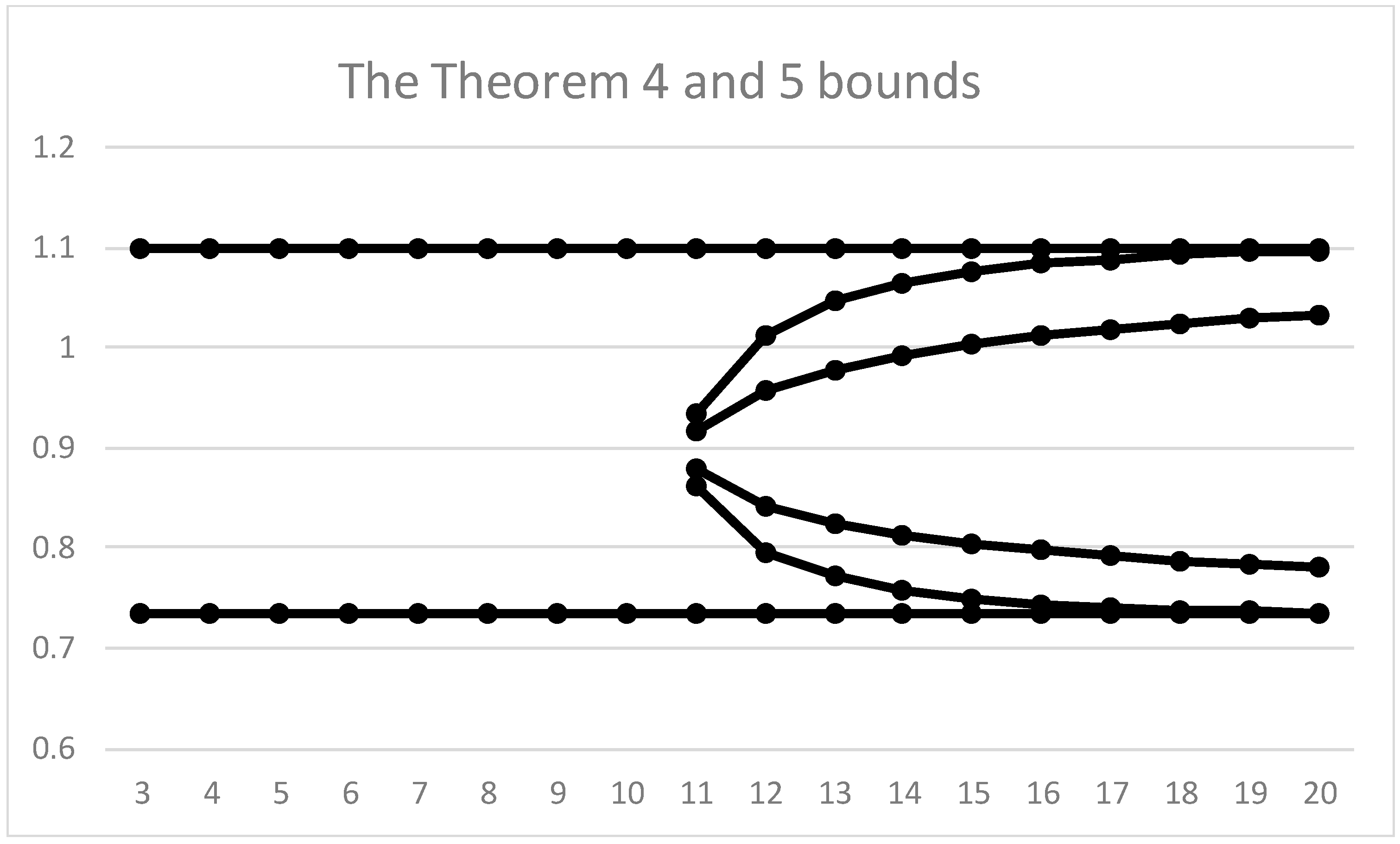
- (i)
- If , then a has a unique IRR.If , let and be the larger and smaller of roots of the quadratic in (1) above, let the quantities be as defined as in (3) above, where r can be either or , and let the transaction b() be defined as in Equation (2) above for 0 . Then,
- (ii)
- If < , then a has a unique IRR, and this must be less than the smallest IRR of b(.
- (iii)
- If < < ), then a must have three IRRs: one less than − 1: one strictly between − 1 and − 1, and one strictly greater than − 1. Moreover, the smallest IRR must be greater than the smallest IRR of b(, and the largest IRR must be less than the largest IRR of b(.
- (iv)
- If > , then a has a unique IRR, and this must be greater than the largest IRR of b(.
- (i)
- If the extremal transaction a has an IRR which is less than the smallest IRR of b( , then a has a unique IRR.
- (ii)
- If the extremal transaction a has an IRR which lies between the smallest IRR of b(and the largest IRR of b(, then a has three IRRs, and they all lie in this range.
- (iii)
- If the extremal transaction a has an IRR which is larger than the largest IRR of b(, then a has a unique IRR.
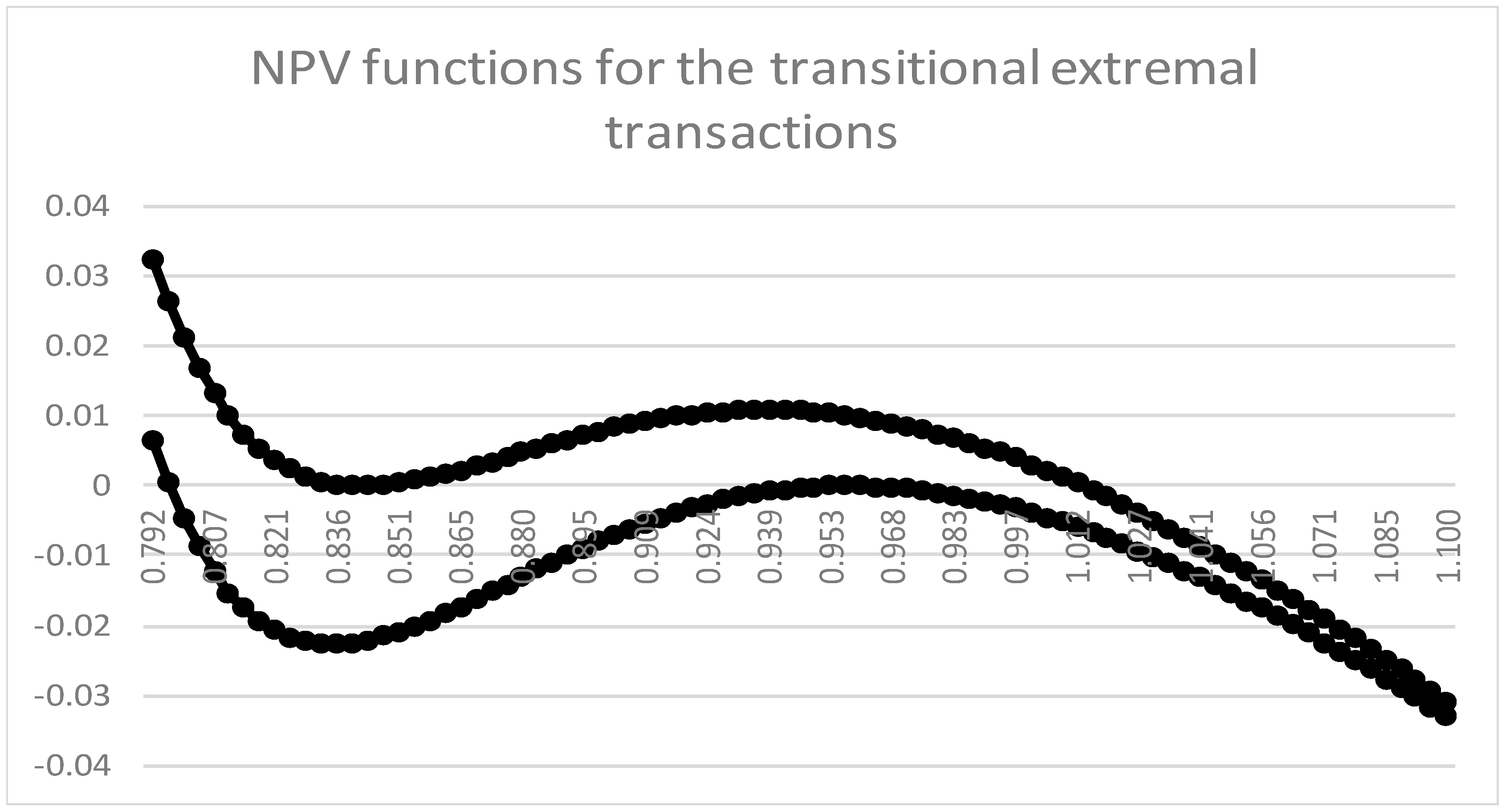
- (i)
- The extremal transaction defined as above, has an IRR at .
- (ii)
- For each u satisfying < u < , it holds that
- (iii)
- For each u satisfying < u < , it holds that
- (i)
- If a has an IRR such that is less than the smallest IRR of b( , then is the unique IRR of a.
- (ii)
- If a has an IRR such that is greater than the largest IRR of b( , then is the unique IRR of a.
5. Further Results Regarding the Distribution of IRRs
- (i)
- a can have no more than one IRR such that
- (ii)
- a has at least one IRR such that
6. An Open Question
- (i)
- Is it possible to develop a lower bound for as a function of n and r?And, more specifically,
- (ii)
- The formula holds for r = 3 and r = n (and trivially for r = 1). Does this formula hold for r = 5 to (n − 1)?
7. Conclusions
- As shown in the paper by Magni and Cuthbert (2018), the unique partition, in conjunction with Magni’s concept of the average internal rate of return, can be used to define a pure investment average internal rate of return (PIAIRR). The PIAIRR is a good candidate for a reliable money-weighted rate of return which may be used by practitioners in assessing investment performance.
Funding
Data Availability Statement
Conflicts of Interest
Appendix A
- (i)
- Proof of Lemma 1:
b − (n − 1)c + nd = −ε, where ε = NPV′(a, 0)
bc = τad
- (1)
- If < 0, then < , or > .
- (2)
- If = 0, then = or .
- (3)
- If > 0, then < < .
- (ii)
- Proof b() has an IRR equal to − 1.
- (iii)
- Proof of Lemma 2.
- (iv)
- Proof of Theorem 4.
- (v)
- Proof of Lemma 3.
Appendix B
- Proof of Theorem 6.
- Proof of Theorem 7.
Appendix C
References
- Cuthbert, James Rutherford. 2018. Partitioning Transaction Vectors into Pure Investments. The Engineering Economist 63: 143–57. [Google Scholar] [CrossRef]
- Cuthbert, James Rutherford. 2021. Sequel to “Partitioning Transaction Vectors into Pure Investments”: A New Sufficient Condition for Transactions to have a Unique IRR; and Some Results on the Distribution of IRRs. The Engineering Economist 66: 303–18. [Google Scholar] [CrossRef]
- Gronchi, Sandro. 1986. On investment criteria based on the internal rate of return. Oxford Economic Papers 38: 174–80. [Google Scholar] [CrossRef]
- Hartman, Joseph C., and Ingrid C. Schafrick. 2004. The relevant internal rate of return. The Engineering Economist 49: 139–58. [Google Scholar] [CrossRef]
- Hazen, Gordon B. 2003. A new perspective on multiple internal rates of return. The Engineering Economist 48: 31–51. [Google Scholar] [CrossRef]
- Magni, Carlo Alberto. 2010. Average rate of return and investment decisions: A new perspective. The Engineering Economist 55: 150–81. [Google Scholar] [CrossRef]
- Magni, Carlo Alberto. 2013. The Internal-Rate-of-Return approach and the AIRR paradigm: A refutation and a corroboration. The Engineering Economist 58: 73–111. [Google Scholar] [CrossRef]
- Magni, Carlo Alberto, and James R. Cuthbert. 2018. Some problems of the IRR in measuring investment performance, and how to solve these with the pure investment AIRR. Journal of Performance Measurement 22: 39–50. [Google Scholar]
- Osborne, Michael J. 2010. A resolution to the NPV-IRR debate? The Quarterly Review of Economics and Finance 50: 234–39. [Google Scholar] [CrossRef]
- Pierru, Axel. 2010. The simple meaning of complex rates of return. The Engineering Economist 55: 105–17. [Google Scholar] [CrossRef]
- Soper, Charles S. 1959. The Marginal Efficiency of Capital: A Further Note. The Economic Journal 69: 174–77. [Google Scholar] [CrossRef]
Disclaimer/Publisher’s Note: The statements, opinions and data contained in all publications are solely those of the individual author(s) and contributor(s) and not of MDPI and/or the editor(s). MDPI and/or the editor(s) disclaim responsibility for any injury to people or property resulting from any ideas, methods, instructions or products referred to in the content. |
© 2023 by the author. Licensee MDPI, Basel, Switzerland. This article is an open access article distributed under the terms and conditions of the Creative Commons Attribution (CC BY) license (https://creativecommons.org/licenses/by/4.0/).
Share and Cite
Cuthbert, J.R. The Use of the Partitioning Theorem to Prove Further Results Regarding the Distribution of IRRs: And an Open Question. J. Risk Financial Manag. 2023, 16, 348. https://doi.org/10.3390/jrfm16080348
Cuthbert JR. The Use of the Partitioning Theorem to Prove Further Results Regarding the Distribution of IRRs: And an Open Question. Journal of Risk and Financial Management. 2023; 16(8):348. https://doi.org/10.3390/jrfm16080348
Chicago/Turabian StyleCuthbert, James Rutherford. 2023. "The Use of the Partitioning Theorem to Prove Further Results Regarding the Distribution of IRRs: And an Open Question" Journal of Risk and Financial Management 16, no. 8: 348. https://doi.org/10.3390/jrfm16080348
APA StyleCuthbert, J. R. (2023). The Use of the Partitioning Theorem to Prove Further Results Regarding the Distribution of IRRs: And an Open Question. Journal of Risk and Financial Management, 16(8), 348. https://doi.org/10.3390/jrfm16080348